Article

On the Stability of Rubble Mound Structures under Oblique Wave Attack

by
Meysam Bali
1,
Amir Etemad-Shahidi
2,3,* and
Marcel R. A. van Gent
4,5
1
Pouya Tarh Pars Consulting Company, Tehran 1437615613, Iran
2
Griffith School of Engineering and Built Environment, Griffith University, Mount Gravatt, QLD 4222, Australia
3
School of Engineering, Edith Cowan University, Joondalup, WA 6027, Australia
4
Department of Coastal Structures & Waves, Deltares, 2600 MH Delft, The Netherlands
5
Department of Hydraulic Engineering, Delft University of Technology (TU Delft), 2628 CN Delft, The Netherlands
*
Author to whom correspondence should be addressed.
J. Mar. Sci. Eng. 2023, 11(7), 1261; https://doi.org/10.3390/jmse11071261
Submission received: 30 April 2023 / Revised: 31 May 2023 / Accepted: 15 June 2023 / Published: 21 June 2023
(This article belongs to the Special Issue Coastal Engineering: Sustainability and New Technologies, 2nd Edition)

Abstract

:
Slope stability formulae for rubble mound structures are usually developed for head-on conditions. Often, the effects of oblique waves are neglected, mainly because it is assumed that for oblique wave attack, the reduction in damage compared to perpendicular wave attack is insignificant. When the incident waves are oblique, the required armour size can be reduced compared to the perpendicular wave attack case. Therefore, it is important to consider the wave obliquity influence on slope stability formulae as a reduction factor. One of the most recent formulae for estimating the stability of rock-armoured slopes, referred to as Etemad-Shahidi et al. (2020), was proposed for perpendicular wave attack. The aim of this study is to develop a suitable wave obliquity reduction factor for the above-mentioned stability formula. To achieve this, first, laboratory experiment datasets from existing reliable studies were selected and analysed. Then, previously suggested reduction factors were evaluated and a suitable reduction factor for the mentioned stability formula were suggested. The suggested reduction factor includes the effect of wave obliquity and directional spreading explicitly. It is shown that the stability prediction is improved by using the wave obliquity reduction factor.

1. Introduction

Many studies are being conducted on breakwaters and especially new breakwaters [1,2,3,4,5,6,7]. However, studies in the field of rubble mound breakwaters have not stopped yet, and many studies are still being conducted in different fields of rubble mound breakwaters [8,9,10,11]. One of the most important issues in breakwater design is the determination of the armour block’s weight using the stability number Ns. Stability formulae for armour layers of rubble mound structures are typically based on laboratory experiments in wave flumes, i.e., 2D experiments. Therefore, the formulae are generally developed for perpendicular wave attack and do not include effects of oblique waves. This is, however, a conservative assumption since the stability of armour slopes generally increases for oblique waves. Waves usually attack breakwater obliquely, and it is important to find out how much the stability increases due to the wave obliquity. Oblique wave attack does not only affect the stability of armour layers, but also wave overtopping. To account for the effects of oblique waves on mean overtopping discharges, several studies have been conducted [12,13,14,15,16]. In most of them, a reduction factor for wave obliquity has been proposed to mean overtopping discharges.
Several studies have been performed to investigate the effect of wave angle (β) on armour stability. A few researchers have performed laboratory experiments to consider effects of oblique waves on the stability of armour layers. They performed tests with long-crested and/or short-crested waves on rock and/or concrete armour layers. Almost all test results showed that for oblique waves, smaller units are required. Therefore, they proposed a reduction factor (γβ) in the required armour size. This reduction factor has been found to be a function of (cosXβ). Galland [13] carried out tests with long-crested waves and incident waves with angles between β = 0° and 75° and proposed X = 0.25. Yu et al. [17] performed tests with long-crested and short-crested waves with angles between β = 0° and 60° on rock and suggested X = 1.16. Wolters and Van Gent [18] also provided a dataset for wave angles up to β = 70° for rock and they obtained X = 1.1, which is very close to that suggested by Yu et al. [17]. In the last study, Van Gent [19] performed small-scale tests in a wave basin to assess the effects of oblique waves on the stability of rock slopes and armoured cubes. The physical model experiments were focused on wave directions between perpendicular (0°) and parallel (90°) using both short- and long-crested waves. They showed that that for rock slopes, the influence of oblique waves is larger for long-crested waves. Table 1 shows the wave obliquity reduction factor for rock armour stability from various authors. This table shows that Galland [13] indicates a much smaller influence of wave obliquity compared to other studies. Moreover, in the approach by Van Gent [19], a minimum value for the reduction factor was suggested for parallel waves with wave angle of 90°. In fact, when waves are parallel to the longitudinal axis of the structure, the reduction factor is limited to 0.42 and 0.35 for short-crested and long-crested waves, respectively.
Figure 1 shows the graphical presentation of wave obliquity reduction factor suggested in different references. As discussed before, Galland [13] indicates the lower influence of wave obliquity. In the range of 0 < β < 45, the prediction of wave obliquity reduction factor by Yu et al. [17], Wolters and Van Gent [18] (WV) and Van Gent [19] (VG) are very similar, and for angles more than 50° degrees, they become different. For β > 45, Yu et al. [17] and WV predict a much higher influence of the wave obliquity on armour size than that of Van Gent [19] for rock slopes.
There are several experimental formulae for the predication of stability number [1,20,21,22,23]. They have been generally developed for perpendicular wave attack without considering the wave obliquity effects. The suggested reduction factors (γβ) are compatible with a specific stability formula. For example, the formula proposed by Yu et al. [17] is compatible with Hudson’s [20] stability formula, i.e.:
N s = H s Δ D n 50 = K D cot α 1 / 3
where Ns is the stability number, Dn50 is the nominal diameter of the stones, Hs is the significant wave height, α is the structure front angle, Δ = ρaw − 1 is the relative buoyant density, ρa is the armour density and ρw is the density of water. The stability coefficient, KD, incorporates the effects of armour type and safety factor, and it varies from 2 (1.6) for breaking waves to 4 (2.8) for non-breaking waves hitting the trunk (head) of a breakwater. Van Gent’s [19] reduction factor is compatible with Van Gent et al.’s [22] rock armour stability formula, i.e.,:
N s = 8.4 P 0.18 I r m 1,0 0.5 ( S d / N w ) 1 / 5 ( H s / H 2 % )    If I r m 1,0 < I r c   or   cot α 4 ( 6 a ) N s = 1.3 P 0.13 I r m 1,0 P cot α 0.5 ( S d / N w ) 1 / 5 ( H s / H 2 % )    If I r m 1 , 0 I r c   and   cot α   < 4 ( 6 b )
with I r c = (6.46P0.31 tanα0.5)1/(P+0.5).
In this equation, P is the permeability, H2% is the average of the highest 2% of incident waves, Sd is the damage level, Nw is the number of waves and I r m 1,0 is the Iribarren number using Tm−1,0 (the spectral mean energy period). Equation (6a,b) were applied for the plunging and surging condition, respectively.
One of the most recent formulae for the calculation of rock stability number is Etemad-Shahidi et al.’s [1], hereafter EBV, shown below:
N s = 3.9 C p N w 1 / 10 S d 1 / 6 I r m 1,0 1 / 3 If   I r m 1 , 0 1.8 ( surging waves ) ( 7 a ) N s = 4.5 C p N w 1 / 10 S d 1 / 6 I r m 1,0 7 / 12 If     I r m 1,0 < 1.8 ( plunging waves ) ( 7 b )
where Cp is the coefficient of permeability defined as [1 + (Dn50c/Dn50)3/10]3/5 and Dn50c is the median nominal size of the core material. An extensive database from different sources was used to develop this formula. Moreover, this formula is based on the local significant wave height and spectral mean energy period of the incident waves. In addition, instead of permeability, it includes effects of the relative size of core material and is more accurate than other formulae [1].
The main aim of this paper is to investigate effect of the wave obliquity/spreading and extending EBV formula by considering the effect of wave angle and spreading coefficient. To achieve this, first, all existing new reduction factors (Galland [13], Yu et al. [17], Wolters and Van Gent [18] and Van Gent [19]) were examined (in combination with the EBV formula).
For this purpose, the Van Gent [19] dataset (170 records) was used for the development of the new reduction factor, and the Yu et al. [17] dataset (70 records) was used for its evaluation.

2. Methodology

All the used tests are cumulative, while stability formulae are generally based on rebuilt tests. Hence, they need to be adjusted to convert cumulative test results to rebuilt ones first. This adjustment can be achieved by adjusting the number of waves (e.g., Van der Meer and Sigurdarson, 2016). For each of the sea states, the SdNw relationship can be calculated using Equation (7a,b). The estimation of Nw1–2, the number of added waves in test 2 (second test in a cumulative test series), which results in the same damage as that of test 1, is required to convert the Nw of a cumulative test to that of a rebuilt one. Basically, Nw1–2 should be added to Nw2 before estimating the damage using stability formulae. For surging waves, Equation (7a) can be written as:
Sd = 0.266 Ns6 Cp6 Nw0.6 Irm−1,02 if Irm−1,0 ≥ 1.8
Sd1~ Ns16  Nw10.6 Ir1m−1,02
Sd1~ Ns26  Nw1–20.6 Ir2m−1,02
Ns16 Nw10.6 Ir1 m−1,02 = Ns26 Nw1–20.6 Ir2 m−1,02
Nw1–2 = (Ns1/Ns2)10 (Ir1 m−1,0/Ir2 m−1,0)20/6 × Nw1
Ns2/Ns1 = k (as Hs2 = k Hs1), and assuming Ir1m−1,0Ir2m−1,0 (constant wave steepness test series), then Nw1–2/Nw1 = (1/k)10. k is commonly about 1.20, i.e., a 20% increase in the wave height in the test series. For 1.10 < k < 1.30, the estimations of Nw1–2/Nw1 and ΔSd are listed in Table 2.
The second row shows that Nw1–2/Nw1 is about 16% (assuming k = 1.2). In other words, the (cumulative) damage in the second test is due to Nw2 + 0.16 Nw1 = 1.16 Nw2.
The last row shows the change in the Sd if the tests were non-cumulative/rebuilt (assuming that Nw1 = Nw2 and noting that Sd ~ Nw0.6). For example, if k = 1.2, then ΔSd = (1 + 0.16)0.6 − 1 = 9.3%. In other words, the damage in the second test is 9.3% more than that in a rebuilt test (with the same number of waves), and Ns would differ about 20%.
The Van der Meer formula [21] can also be applied to such situations via the cumulative damage method, which has been described in Van der Meer [24] and later in the Rock Manual [25], and which has also been implemented in Breakwat. In fact, the method is quite straightforward. The first sea state, characterised by a significant wave height Hs1, mean period Tm1 and number of waves Nw1, yields a calculated damage level Sd1. The second sea state would be defined by HS2, Tm2 and Nw2. The next step is to determine the number of waves (Nw12) required for the second sea state to induce the same level of damage (Sd1) caused by the first sea state. Subsequently, the damage for the second sea state (Sd2) can be calculated by applying (Nw1–2 + Nw2) as the total number of waves.
More discussion about conversion of cumulative-to-rebuilt damage is described in van der Meer and Sigurdarson [26].
After this modification, tests with very low damage levels (Sd < 2) and very high damage levels (Sd > 12), which are less common in practice [25,27] (e.g., Rock Manual, 2007, CEM, 2011), were excluded. In this way, a total of 77 records were selected for further processing. A brief description of the range of governing parameters based on β (0°, 15°, 30°, 45°, 60°, 70°, 80° and 90°) and S (0, 10, 25 and 40) ranges is presented in Table 3 and Table 4, respectively. Note that for the tests with directional spreading, the amount of directional spreading is described by S, where S = 0 corresponds to long-crested waves.

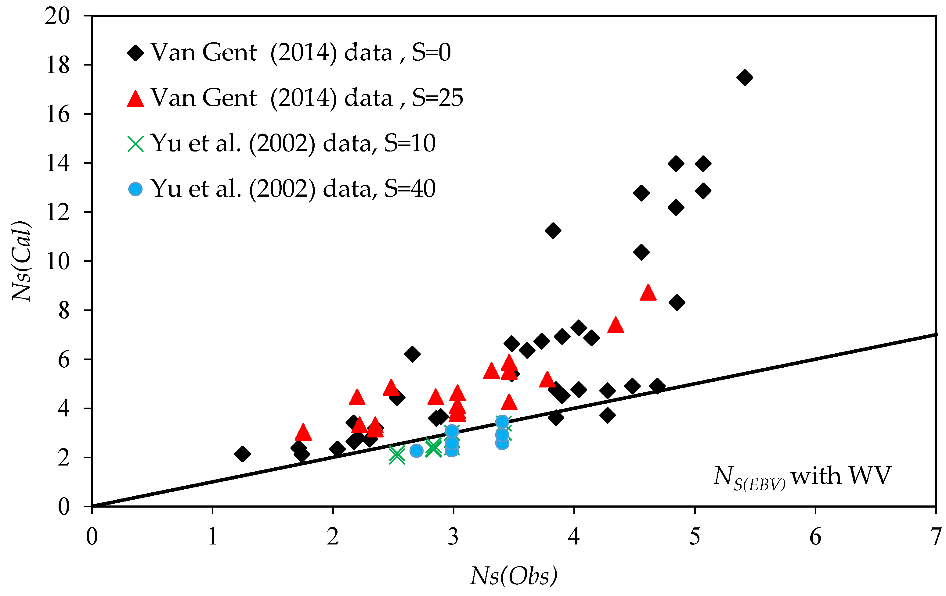
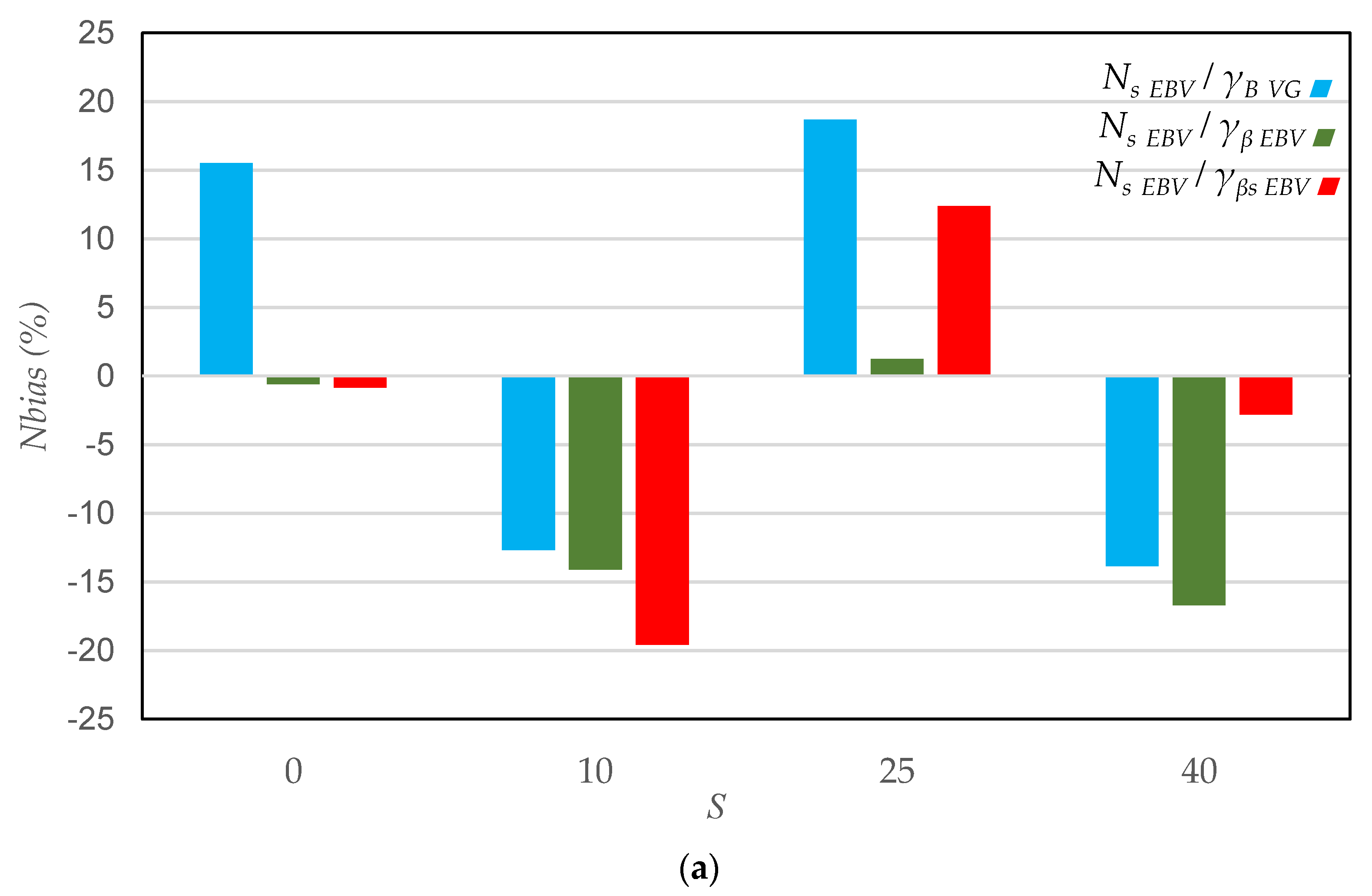
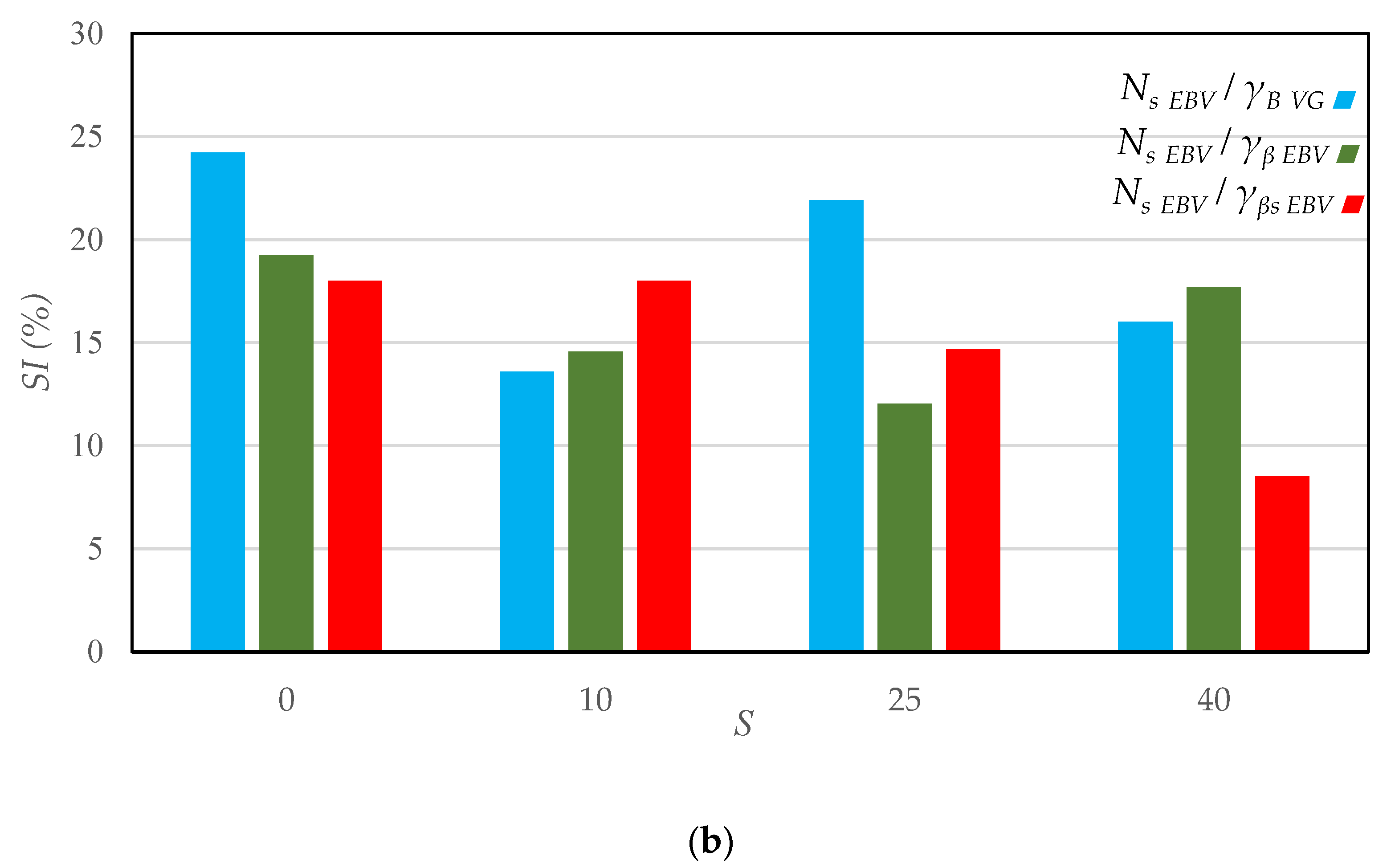
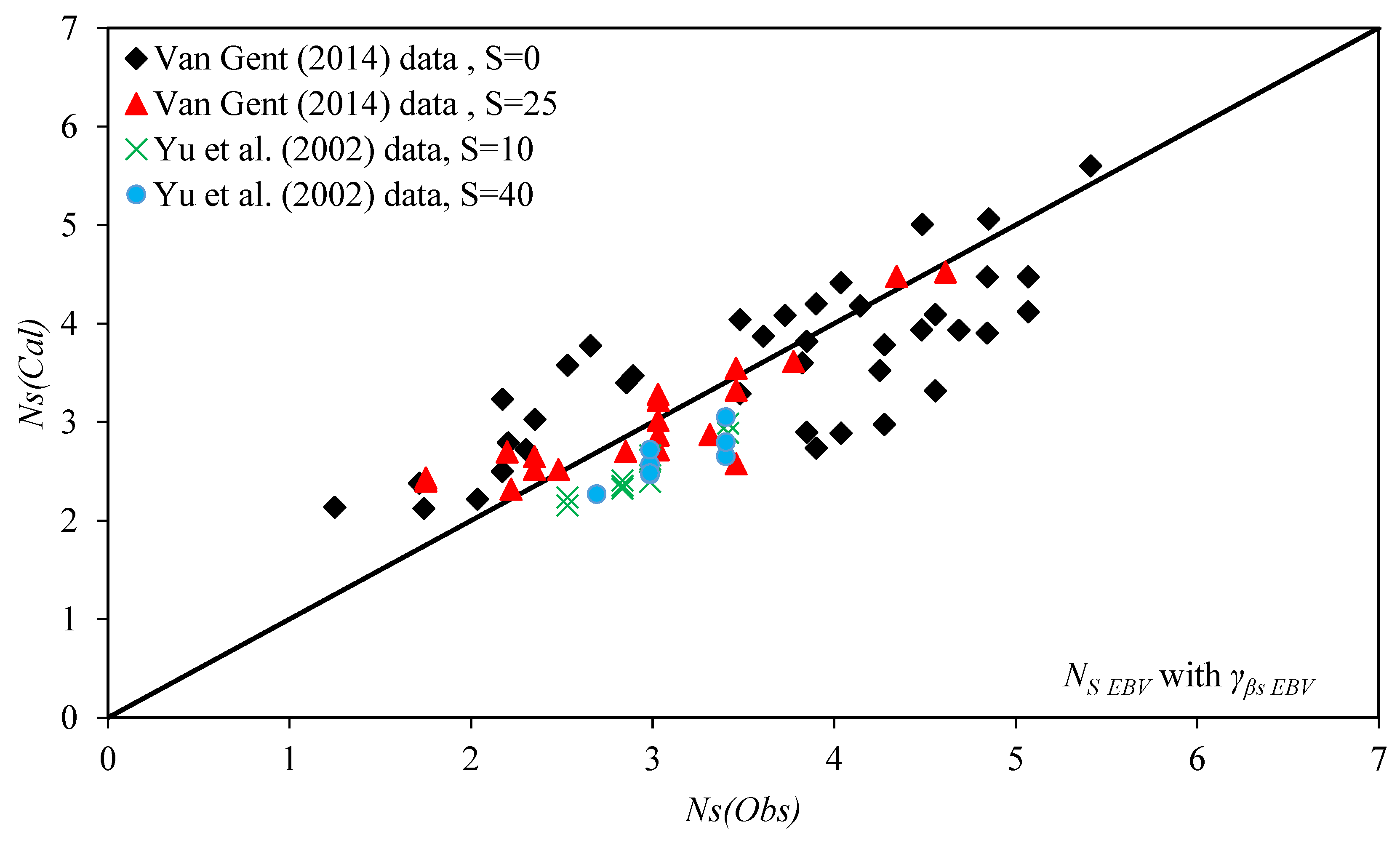
3. Results and Discussion

First, the Galland [13], Yu et al. [17], Wolters and Van Gent [18] and Van Gent [19] reduction functions in combination with the EBV stability formula were evaluated. Then, an attempt was made to find an appropriate and compatible reduction factor for the EBV stability formula. Figure 2, Figure 3, Figure 4 and Figure 5 show the comparison of observed and predicted stability numbers using existing reduction factors. As seen, the Van Gent [9] one is more appropriate compared to the other reduction factors. As discussed before and shown in Figure 1, for β > 45, Yu et al. [17] and WV predict a much higher influence of the wave obliquity on rock size (reduction in armour size) and stability number (increase in the stability number) compared to Van Gent [19].
Next, we attempted to derive a compatible reduction factor for applications in combination with the EBV stability formula.
Figure 6a shows that the f(β) = Ns EBV/Ns Measured versus β. As seen Ns EBV/Ns Measured is scattered. For example, Ns EBV/Ns Measured is between 0.4 and 0.8 for β = 60°. Moreover, some records for relatively small wave angles and long-crested waves (S = 0) result in reduction factors larger than 1, and some data points at β = 0° are not close to 1. The values larger than 1 for perpendicular waves are due to differences between the stability expression and the data. The data point with a gamma value larger than 1 for a wave angle of 15 degrees, larger than for perpendicular waves, is based on low damage values (Sd = 2.2 for perpendicular waves). For low damage values, there is a natural larger relative spreading in the results due to the dependency of the damage values on the (in)stability of only a few stones.
It should be mentioned that this is not because of using NS EBV for stability; the issue exists when using other stability formulae. For example, in Figure 6b, the VSK formula was applied and data points at β = 0° are not close to 1. It was found that to derive a more appropriate and compatible reduction factor for the EBV stability formula, the Van Gent [19] reduction function can be used with a modified cβ value. Using the Van Gent [19] approach, the optimal cβ values are 0.54 and 0.44 for short- and long-crested waves, respectively. Therefore, the reduction factor for the EBV stability formula can be proposed to be:
γβ EBV = (1 − cβ) cos2β + cβ       cβ = 0.44 (0.54) for long (short) crested waves
Figure 6a shows the comparison of Van Gent [19] and the reduction factor calibrated for the EBV formula versus β. As seen, using a modified cβ for application in combination with the EBV stability expression indicates less influence of wave obliquity compared to that suggested by Van Gent [19] in combination with another stability formula.
Figure 7 shows the comparison between the measured and predicted stability numbers using the new wave obliquity reduction factor. As seen, the scatter in the data is reduced in this way. In addition, most of the data points are concentrated on the line of the perfect agreement when using EBV with a new reduction factor predicts the stability much better than others’ formulae.
The performances of the various formulae were also evaluated quantitatively using accuracy metrics such as the normalised bias (NBias), the scatter index (SI) and the correlation coefficient (CC), defined below:
N B i a s = 1 n 1 n ( p i m i ) m ¯ i × 100
S I = 1 n i = 1 n ( p i m i ) 2 m ¯ i × 100
C C = i = 1 n ( p i p i ¯ ) ( m i m i ¯ ) i = 1 n ( m i m i ¯ ) 2 ( p i p i ¯ ) 2
where pi and mi denote the predicted and measured values, respectively. The number of measurements is n and the bar denotes the mean value.
Table 5 and Table 6 display the accuracy metrics of the EBV stability formula using Van Gent [19] and the new reduction factor based on the Van Gent [19] and Yu et al. [17] datasets, respectively. As seen, the calibration of the coefficient in Equation (13) results in a negligible bias.
As seen, the new suggested reduction factor (γβ EBV) considers the effect of wave angle (quantitatively) and wave spreading for short- and long-crested waves (qualitatively). Therefore, in the third step, a reduction coefficient (γβsEBV), which is a function of wave angle and spreading qualitatively, will be investigated.
As discussed in Yu et al. [17] and Van Gent [19], unidirectional (long-crested) and multidirectional (short-crested) oblique waves can affect the stability number differently. They concluded that more spreading leads to reducing the influence of wave obliquity. Here, the effects of wave directionality were reanalysed. Experiments by Yu et al. [17] included only tests with S = 10 and S = 40 as a measure for directional spreading. The usual minimum and maximum values of wave spreading are 0 and about 45, respectively. These extreme values are covered in the used datasets but with no intermediate values. Based on the available data, a linear function can be proposed for the estimation of cβ as a function of S, i.e., cβ = 0.44 + 0.004S (γβsEBV = (1 − cβ) cos2β + cβ). This means that cβ varies linearly between 0.44 for S = 0 and 0.60 for S = 40. In other words, the more spreading, the smaller the effect of wave obliquity, which is physically sound as more spreading means that waves are coming from different directions. As seen, γβsEBV considers the quantitative effect of wave angle and wave spreading.
The accuracy metrics of this reduction factor for different datasets are shown in the last column of Table 5 and Table 6. As seen, the proposed formula provides reasonable results for considering wave spreading in oblique waves. For more investigation, the accuracy metrics (NBias and SI) of these reduction factors for different range of β and S are shown in the Figure 8 and Figure 9. It can be concluded that the new reduction factor has more accurate prediction in almost all wave angles (except β = 30) and in all wave spreading situations (except S = 10) than others. The accuracy in the prediction is seen also in the Figure 10 and the scatter in the data is reduced in this way.
Figure 11 displays the effects of wave direction and spreading on the reduction in required armour size. As seen, an increase in wave spreading leads to a reduction in required armour size. For example, for a wave angle of 40° and wave spreading of 30, the reduction factor of the armour size is 0.8. Hence, the armour size calculated based on Etemad-Shahidi et al. [1] can be decreased by 20%.

4. Summary and Conclusions

One of the most recent formulae for estimating the stability of rock-armoured slopes is Etemad-Shahidi et al. [1], or EBV. The aim of this study was to develop a suitable wave obliquity reduction factor for the EBV stability formula. Hence, the influence of oblique waves on the stability of the rock armour layer has been investigated based on the available dataset. Data records of Yu et al. [17] and Van Gent [19], with damage levels in the range of 2 ≤ Sd ≤ 12, were selected. These studies show that the influence of oblique waves on the stability of rock armour layers is significant, and the required armour size can be reduced, compared to the perpendicular wave attack case. This effect can be considered the reduction factor γβ for the required armour size which can reduce construction costs. For example, a 15% reduction in armour size will result in about a 40% reduction in the armour’s weight, which is significant.
All available γβ formulae were evaluated in combination with the EBV stability formula using different datasets separately, and it was concluded that the Van Gent [19] approach provides more accurate predictions than the others. Based on their approach, an appropriate and compatible reduction factor for the EBV stability formula was developed, which includes the effect of directional spreading explicitly for the first time. It was concluded that the results are improved slightly by using the new and more physically sound wave obliquity reduction factor.
In this study, one of the most recent formulae for estimating the stability of rock-armoured slopes was extended by considering the effects of the wave angle and the directional spreading coefficient. The results show that the prediction is more accurate and reliable when using an expression calibrated for the mentioned stability formula. The newly proposed reduction formula, γβsEBV = (1 − cβ) cos2β + cβ with cβ = 0.44 + 0.004S, leads to an unbiased prediction and a 30% improvement in SI, with a coefficient of variation of 19%. It should be noted that the effect of wave multi-directionality on stability has been quantified explicitly for the first time.

Author Contributions

M.B.: Conceptualization, Writing—original draft Validation, Formal analysis. A.E.-S.: Conceptualization, Methodology, Writing—review & editing, M.R.A.v.G.: Data curation, Writing—review & editing, Conceptualization. All authors have read and agreed to the published version of the manuscript.

Funding

This research received no external funding.

Institutional Review Board Statement

Not applicable.

Informed Consent Statement

Not applicable.

Data Availability Statement

Data are available upon reasonable request.

Conflicts of Interest

The authors declare no conflict of interest.

Nomenclature

SymbolNameUnit
αStructure slope angle[°]
βWave angle[°]
CPPermeability coefficient[-]
CCCorrelation coefficient [-]
∆ = (ρsw) − 1Relative buoyant mass density[-]
Dn50 = (M50/ρa)1/3Armour equivalent cube length exceeded by 50% of a sample by weight [m]
D50Equivalent spherical diameter[m]
Dn50cCore equivalent cube length exceeded by 50% of a sample by weight[m]
EBVEtemad-Shahidi et al. [1][-]
γβ EBVNew wave angle and spreading reduction factor which is a function of β (quantitatively) and S (qualitatively) for EBV formula[-]
γβS EBVNew wave angle and spreading reduction factor which is a function of β (quantitatively) and S (quantitatively) for EBV formula[-]
γBVGWave angle and spreading reduction factor suggested by Van Gent [19][-]
Hm0Significant wave height based on frequency domain analysis[m]
H2%Average of the highest 2% of incident waves[m]
H50Average of the 50 highest waves [m]
HsSignificant wave height at toe of the structure[m]
hWater depth
KDHudson stability coefficient[-]
Irm−1,0Iribarrn number based on Tm−1,0.[-]
IrcTransition Iribarrn number in VSK formula[-]
miMeasured values[-]
m i ¯ Average of the measured values[-]
M50Median rock mass[kg]
nThe number of observations[-]
NwNumber of wave attack[-]
NsStability number using Hs[-]
NS EBVStability number calculated by EBV formula[-]
NS VSKStability number calculated by VSK formula[-]
Ns MeasuredMeasured stability number
N50Stability number using H50[-]
PNominal permeability[-]
PiPredicted values[-]
RcCrest freeboard [m]
ρsRock density[kg/m3]
ρwWater density[kg/m3]
Som = 2πHmo/gTom2Deep water wave steepness using Tom[-]
Som−1,0Deep water mean wave steepness using T−1,0[-]
SdDamage level[-]
SIScatter index[-]
Tm−1,0 = m−1/m0Mean energy wave period based on frequency domain [s]
TPPeak wave period[s]
TmMean wave period[s]
Tm−1,0,deepMean energy wave period based on frequency domain analysis in deep water[s]
VSKVan Gent et al. [22][-]
VGVan Gent [19]
WVWolters and Van Gent [18][-]

References

  1. Etemad-Shahidi, A.; Bali, M.; van Gent, M.R.A. On the stability of rock armored rubble mound structures. Coast. Eng. 2020, 158, 103655. [Google Scholar]
  2. Kolahdoozan, M.; Bali, M.; Rezaee, M.; Moeini, M.H. Wave-transmission prediction of π-type floating breakwaters in intermediate waters. J. Coast. Res. 2017, 33, 1460–1466. [Google Scholar] [CrossRef]
  3. Han, M.; Wang, C. Hydrodynamics study on rectangular porous breakwater with horizontal internal water channels. J. Ocean Eng. Mar. Energy 2020, 6, 377–398. [Google Scholar] [CrossRef]
  4. Wang, C.M.; Han, M.M.; Lyu, J.; Duan, W.H.; Jung, K.H.; Kang An, S. Floating forest: A novel concept of floating breakwater-windbreak structure. In WCFS2019: Proceedings of the World Conference on Floating Solutions; Springer: Singapore, 2020; pp. 219–234. [Google Scholar]
  5. Rahman, S.; Baeda, A.; Achmad, A.; Jamal, R. Performance of a New Floating Breakwater. In IOP Conference Series: Materials Science and Engineering; IOP Publishing: Bristol, UK, 2020; p. 012081. [Google Scholar]
  6. Zhu, Y.; Tang, H. Automatic Damage Detection and Diagnosis for Hydraulic Structures Using Drones and Artificial Intelligence Techniques. Remote Sens. 2023, 15, 615. [Google Scholar] [CrossRef]
  7. Gao, J.; Ma, X.; Dong, G.; Chen, H.; Liu, Q.; Zang, J. Investigation on the effects of Bragg reflection on harbor oscillations. Coast. Eng. 2021, 170, 103977. [Google Scholar] [CrossRef]
  8. Karimaei Tabarestani, M.; Feizi, A.; Bali, M. Reliability-based design and sensitivity analysis of rock armors for rubble-mound breakwater. J. Braz. Soc. Mech. Sci. Eng. 2020, 42, 136. [Google Scholar] [CrossRef]
  9. Etemad-Shahidi, A.; Bali, M.; van Gent, M.R.A. On the toe stability of rubble mound structures. Coast. Eng. 2021, 164, 103835. [Google Scholar] [CrossRef]
  10. Etemad-Shahidi, A.; Koosheh, A.; van Gent, M.R.A. On the mean overtopping rate of rubble mound structures. Coast. Eng. 2022, 177, 104150. [Google Scholar] [CrossRef]
  11. Houtzager, D.; Hofland, B.; Caldera, G.; van der Lem, C.; van Gent, M.; Bakker, P.; Antonini, A. Embedded rocking measurement of single layer armour units: Development and first results. In Proceedings of the ICE Breakwaters 2023: Coasts, Marine Structures and Breakwaters, Portsmouth, UK, 25–27 April 2023. [Google Scholar]
  12. De Waal, J.; Van der Meer, J. Wave runup and overtopping on coastal structures. In Proceedings of the 23rd International Conference on Coastal Engineering, Venice, Italy, 4–9 October 1992; pp. 1758–1771. [Google Scholar]
  13. Galland, J.-C. Rubble mound breakwater stability under oblique waves: An experimental study. In Proceedings of the 24th International Conference on Coastal Engineering, Kobe, Japan, 23–28 October 1994; pp. 1061–1074. [Google Scholar]
  14. Hebsgaard, M.; Sloth, P.; Juhl, J. Wave overtopping of rubble mound breakwaters. In Proceedings of the 26th International Conference on Coastal Engineering, Copenhagen, Denmark, 22–26 June 1998; pp. 2235–2248. [Google Scholar]
  15. Andersen, T.L.; Burcharth, H.F. Three-dimensional investigations of wave overtopping on rubble mound structures. Coast. Eng. 2009, 56, 180–189. [Google Scholar] [CrossRef]
  16. Nørgaard, J.Q.H.; Andersen, T.L.; Burcharth, H.F.; Steendam, G.J. Analysis of overtopping flow on sea dikes in oblique and short-crested waves. Coast. Eng. 2013, 76, 43–54. [Google Scholar] [CrossRef]
  17. Yu, Y.-X.; Liu, S.-X.; Zhu, C.-H. Stability of armour units on rubble mound breakwater under multi-directional waves. Coast. Eng. J. 2002, 44, 179–201. [Google Scholar] [CrossRef]
  18. Wolters, G.; Van Gent, M. Oblique wave attack on cube and rock armoured rubble mound breakwaters. Coast. Eng. Proc. 2011, 32, 34. [Google Scholar] [CrossRef] [Green Version]
  19. Van Gent, M.R.A. Oblique wave attack on rubble mound breakwaters. Coast. Eng. 2014, 88, 43–54. [Google Scholar] [CrossRef]
  20. Hudson, R. Design of Quarry-Stone Cover Layers for Rubble-Mound Breakwaters; Coastal Engineering Research Centre: Vicksburg, MS, USA, 1958. [Google Scholar]
  21. Van der Meer, J.W. Deterministic and probabilistic design of breakwater armor layers. J. Waterw. Port Coast. Ocean Eng. 1988, 114, 66–80. [Google Scholar] [CrossRef]
  22. Van Gent, M.R.A.; Smale, A.J.; Kuiper, C. Stability of rock slopes with shallow foreshores. In Proceedings of the Coastal Structures 2003, Portland, OR, USA, 26–30 August 2003; pp. 100–112. [Google Scholar]
  23. Etemad-Shahidi, A.; Bali, M. Stability of rubble-mound breakwater using H50 wave height parameter. Coast. Eng. 2012, 59, 38–45. [Google Scholar] [CrossRef] [Green Version]
  24. Van der Meer, J. Stability of rubble mound revetments and breakwaters. In Developments in Breakwaters; ICE Publishing: London, UK, 1985; pp. 191–202. [Google Scholar]
  25. The Rock Manual. The Use of Rock in Hydraulic Engineering. CIRIA-CUR, Publication C683. 2007. Available online: https://www.kennisbank-waterbouw.nl/DesignCodes/rockmanual/introduction.pdf (accessed on 31 May 2023).
  26. Sigurdarson, S.; van der Meer, J. Design and Construction Aspects of Berm Breakwaters. In Coastal Structures and Solutions to Coastal Disasters 2015: Resilient Coastal Communities; American Society of Civil Engineers: Reston, VA, USA, 2017; pp. 864–875. [Google Scholar]
  27. U.S. Army Corps of Engineers. Coastal Engineering Manual (CEM), Engineer Manual 1110-2-1100, 2002, Washington, DC (6 volumes) 2011: US. Chapter VI, Part 5. Available online: https://www.publications.usace.army.mil/USACE-Publications/Engineer-Manuals/u43544q/636F617374616C20656E67696E656572696E67206D616E75616C/ (accessed on 30 April 2023).
Figure 1. Comparison of methods describing the influence of oblique waves on armour size. Red and blue line: Van Gent [19], black line: Galland [13], yellow line: Yu et al. [17] and green line: Wolters and Van Gent [19].
Jmse 11 01261 g001
Figure 2. Comparison between measured and calculated stability number using EBV with Galland reduction factors. Black diamond and red triangle: Van Gent [19], green multiplication and blue circle: Yu et al. [17].
Jmse 11 01261 g002
Figure 3. Comparison between measured and calculated stability number using EBV with Yu et al. [17] reduction factors. Black diamond and red triangle: Van Gent [19], green multiplication and Blue circle: Yu et al. [17].
Jmse 11 01261 g003
Figure 4. Comparison between measured and calculated stability number using EBV with Wolters and Van Gent [18] reduction factors. Black diamond and red triangle: Van Gent [19], green multiplication and blue circle: Yu et al. [17].
Jmse 11 01261 g004
Figure 5. Comparison between measured and calculated stability number using EBV with Van Gent [19] reduction factors. Black diamond and red triangle: Van Gent [19], green multiplication and blue circle: Yu et al. [17].
Jmse 11 01261 g005
Figure 6. (a) Variation in f(β)EBV versus β, (b) variation in f(β)VSK versus β. Black diamond, red triangle: Van Gent [19].
Jmse 11 01261 g006
Figure 7. Comparison between measured and predicted (by EBV) stability numbers using the new reduction factor (γβ EBV). Black diamond and red triangle: Van Gent [19], green multiplication and Blue circle: Yu et al. [17].
Jmse 11 01261 g007
Figure 8. Accuracy metrics of NS EBV using the new and Van Gent [19] wave obliquity reduction factors for different ranges of β in the expressions by EBV, (a) NBias and (b) SI.
Jmse 11 01261 g008aJmse 11 01261 g008b
Figure 9. Accuracy metrics of NS EBV using the new and Van Gent [19] wave obliquity reduction factors for different ranges of S in the expressions by EBV, (a) NBias and (b) SI.
Jmse 11 01261 g009aJmse 11 01261 g009b
Figure 10. Comparison between measured and predicted (by EBV) stability numbers using the new reduction factor (γβs EBV). Black diamond and red triangle: Van Gent [19], green multiplication and blue circle: Yu et al. [17].
Jmse 11 01261 g010
Figure 11. Reduction factor of armour size due to the wave obliquity and different spreading values.
Jmse 11 01261 g011
Table 1. Wave obliquity reduction factor for rock armour size from various studies.
ReferenceFormulaEquation No
Galland [13]cos0.25 β(1)
Yu et al. [17]cos1.157 β(2)
Wolters and Van Gent [18]cos1.1 β(3)
Van Gent [19](1 − cβ) cos2β + cβcβ = 0.42 for short-crested(4)
cβ = 0.35 for long-crested
Table 2. The relation of Nw1–2/Nw1 and ΔSd by assuming Nw1 = Nw2 and Ir1m−1,0Ir2m−1,0.
k1.101.151.201.251.30
Nw1–2/Nw1 (%)392516117
ΔSd (%)21.614.39.36.54
Table 3. Range of parameters used for formula development based on the β range.
Parameter β
015304560708090
Nw10001000100010001000100010001000
cotα1.51.51.51.51.5, 21.5, 21.5, 21.5
D1.71.71.71.71.71.71.71.7
S0–400–400–400–400–400–250–250–25
P0.4, 0.50.4, 0.50.4, 0.50.1–0.50.1–0.50.1–0.50.1–0.50.1–0.5
som−1,0
(×10−2)
3–63–63–63–63–63–63–63–6
Irm−1,02.7–3.62.6–3.62.6–3.52.6–3.62.2–3.72.3- 4.02.2–3.03.1–3.5
h/Hs3.4–10.53.0–14.73–8.02.6–11.02.4–14.52.7–11.34.6–6.55.5–5.9
Dn50c /Dn500.4–0.430.4–0.430.4–0.430–0.430–0.430–0.430–0.430.0–0.43
Sd2–7.12.2–11.52.3–6.52.0–7.02.0–8.82–122.2–9.23.4–3.7
Ns1.7–3.01.2–3.42.3–3.422.0–3.41.7–4.72.2–4.83.8–5.44.2–4.5
Table 4. Range of parameters used for formula development based on the S range.
Parameter S
0102540
Nw1000100010001000
cotα1.5, 21.51.5, 21.5
D1.71.71.71.6
β0–900–4550–700–45
P0.1–0.50.40.1–0.50.4
som−1,0
(×10−2)
3–63–63–63–6
Irm−1,02.2–4.02.6–2.72.2–3.32.6–2.7
h/Hs2.4–14.73.0–4.05.3–14.13–3.76
Dn50c /Dn500.0–0.430.400.0–0.430.40
Sd2–11.52–6.52.3–6.52.1–7.2
Ns1.2–5.42.5–3.42.5–3.42.7–3.4
Table 5. Accuracy metrics of NS EBV using the new and Van Gent [19] wave obliquity reduction factors, Van Gent [17] data.
Ns EBVB VGNs EBV/γβ EBVNs EBV/γβs EBV
NBias16.4−0.05−0.05
SI2417.717.70
CC0.830.800.80
Table 6. Accuracy metrics of NS EBV using the new and Van Gent [19] wave obliquity reduction factors, Yu et al. [17] data.
Ns EBV/γB VGNs EBV/γβ EBVNs EBV/γβs EBV
NBias−13−16.0−15.70
SI1516.8516.10
CC0.770.820.81
Disclaimer/Publisher’s Note: The statements, opinions and data contained in all publications are solely those of the individual author(s) and contributor(s) and not of MDPI and/or the editor(s). MDPI and/or the editor(s) disclaim responsibility for any injury to people or property resulting from any ideas, methods, instructions or products referred to in the content.

