1. Introduction
In the wake of sustained growth within the maritime and shipbuilding industries, the significance of oceanic transport has become increasingly conspicuous. According to estimations by the International Maritime Organization (IMO), approximately 90% of global commerce is conducted via sea transportation [
1]. Nevertheless, ship collision incidents are becoming progressively prevalent. The prevention of inter-ship collisions and the avoidance of surface obstacles are integral components of successful navigation. Statistical data regarding ship collisions reveal that human factors are the primary cause, with approximately 96% of accidents attributed to human error [
2]. In an effort to mitigate such errors, autonomous vessels supporting intelligent navigation have garnered significant interest, with automatic collision avoidance and path planning constituting a pivotal challenge in the development of intelligent ships [
3]. Path-planning technology directly influences the degree of vessel intelligence. In accordance with the International Regulations for Preventing Collisions at Sea (COLREGs) [
4], vessels must continually adapt their collision avoidance and obstacle evasion plans during navigation, adjusting the obstacle trajectory accordingly [
5]. Consequently, it is imperative to investigate a swift and effective path-planning method for implementation in autonomous ship control systems [
6].
Currently, prevalent ship path-planning and collision avoidance algorithms include APF, genetic algorithm (GA) [
7], ant colony optimization (ACO) [
8], particle swarm optimization (PSO), model predictive control, and deep reinforcement learning, among others [
9]. However, these methods have certain limitations in practical applications. For instance, while the APF method is simple and easy to implement, it is prone to local optima [
10]; the GA is suitable for handling complex mathematical models and nonlinear constraint problems but has higher computational complexity [
11]. Consequently, researchers often improve or combine multiple methods to overcome their respective drawbacks and enhance path planning and collision avoidance performance.
Numerous scholars have achieved significant advancements in the fusion and optimization of various path-planning algorithms. Xia Chen et al. [
12] addressed the shortcomings of the rapidly exploring random tree star (RRT*) algorithm, such as slow convergence speed and large randomness in the search range, by proposing a UAV trajectory planning method based on a goal-biased APF-RRT* algorithm. This method employs a goal-biased strategy to guide the generation of random sampling points, accelerating the convergence speed of the algorithm, and introduces an improved APF method into the random search tree to significantly reduce the number of iterations, generate higher quality new nodes, and decrease path length. M. F. D. Santos et al. [
13] addressed the issue of robust control for surface vessels, employing a robust optimal control approach based on continuous loop closure and optimal control theory. They adjusted the PID controller to handle uncertainties arising from different parameter variations. Y. Su et al. [
14] conducted asymptotic dynamic positioning of ships in the presence of constraints on the actuators and partial failures of the actuators. The authors put forth a nonlinear PD fault-tolerant controller. Yangsheng Liu et al. [
15] presented an improved simulated annealing-APF (SA-APF) algorithm to address path-planning problems in 3D space. This method uses the simulated annealing (SA) algorithm to optimize distance costs and combines it with the APF, realizing large-scale multi-objective 3D space path planning. Zhe Zhang et al. [
16] designed a fusion algorithm combining an improved APF method and rolling window method for the local path-planning problem of unmanned underwater vehicles. The rolling window method models the local environment detected by UUV sensors, and the position factor is introduced into the repulsive force equation of the traditional APF method, making the approach effective and real-time. Hang Zhang et al. [
17] developed an adaptive particle swarm optimization APF method. By using the APSO algorithm to preliminarily obtain the global virtual path, the method improves the APF approach and solves the local minimum value problem in traditional APF. Sarada Prasanna Sahoo et al. [
18] proposed a hybrid algorithm combining grey wolf optimization (GWO) and GA and extended the hybrid path-planning to the cooperative path-planning application for autonomous underwater vehicles.
Moreover, numerous scholars have conducted extensive research on dynamic collision avoidance decision algorithms. Yanshuang Du et al. [
19] addressed flight safety issues in dynamic airspace for unmanned aerial vehicles by proposing a real-time reactive collision-free path generation method, capable of adjusting the safe distance based on the relative motion of surrounding obstacles. Wenjun Zhang et al. [
20] examined the relationship between a ship’s encounter state and the COLREGs in the context of collision avoidance for ship path planning, which can help reduce the cost of planned routes. Hongguang Lyu et al. [
21] introduced an autonomous trajectory planning algorithm based on a modified APF, aimed at ensuring that ships or unmanned surface vessels effectively address collision avoidance problems in dynamic environments while adhering to the COLREGs. Yufei Zhuang et al. [
22] proposed a waypoint generation algorithm that considers USV turning radius constraints by establishing an obstacle detection mechanism, reducing redundant turning angles and path lengths when USVs traverse obstacles. They devised a multidimensional path evaluation function for reasonably assessing planned routes, enabling improved USV path planning in complex environments. Zhongxian Zhu et al. [
23] proposed a precise environmental potential field model based on electronic navigational chart (ENC) surface objects and an improved APF, which can obtain collision-free paths under different weather conditions and in narrow waters. Sung-Wook Ohn et al. [
24] considered open-sea, restricted-water interactions between two or multiple vessels and the COLREGs while constructing optimal local path-planning routes for ships.
In practical scenarios, the schematics of ship trajectory planning and collision evasion necessitate a holistic consideration of an array of determinants encompassing vessel dynamics, marine environments, and established navigational safety norms [
1]. Hence, the cruciality of selecting and fine-tuning apt methodologies to circumnavigate real-world dilemmas becomes paramount. The APF algorithm exhibits structural clarity and computational swiftness, making it an indispensable asset in local ship route planning and dynamic obstacle avoidance. Despite the algorithm’s inherent drawbacks in terms of global planning and intricate movements, its theoretical framework is nonetheless amenable to enhancements and pragmatic applications. Further, the synergistic application of the APF and ACO algorithms, particularly if the ACO algorithm can bolster its computational speed and global planning within a broad scale, could offer a more precise resolution to the extensive obstacle path-planning problem. Throughout the research journey, simulation experiments and practical trials can serve as credible tools to authenticate the effectiveness and applicability of the chosen methods, providing invaluable insights for the ongoing study and advancement of intelligent ship navigation.
3. Ship Collision Avoidance Rule Modeling
In open-water navigation, examining ship collision avoidance decision-making and path-planning algorithms requires the integration of the COLREGs as constraints. Key aspects include the following: (1) Feasibility of real-time environmental data collection during navigation and concurrent hazard assessment; (2) Determination of ship collision avoidance decisions, timing, and evasive actions; (3) Consideration of ship dynamics and COLREGs within decision making and trajectory planning.
In compliance with the COLREGs, vessels must ensure that other ships remain outside the safe encounter distance throughout their journey, necessitating navigation beyond the safe encounter distance as a performance criterion.
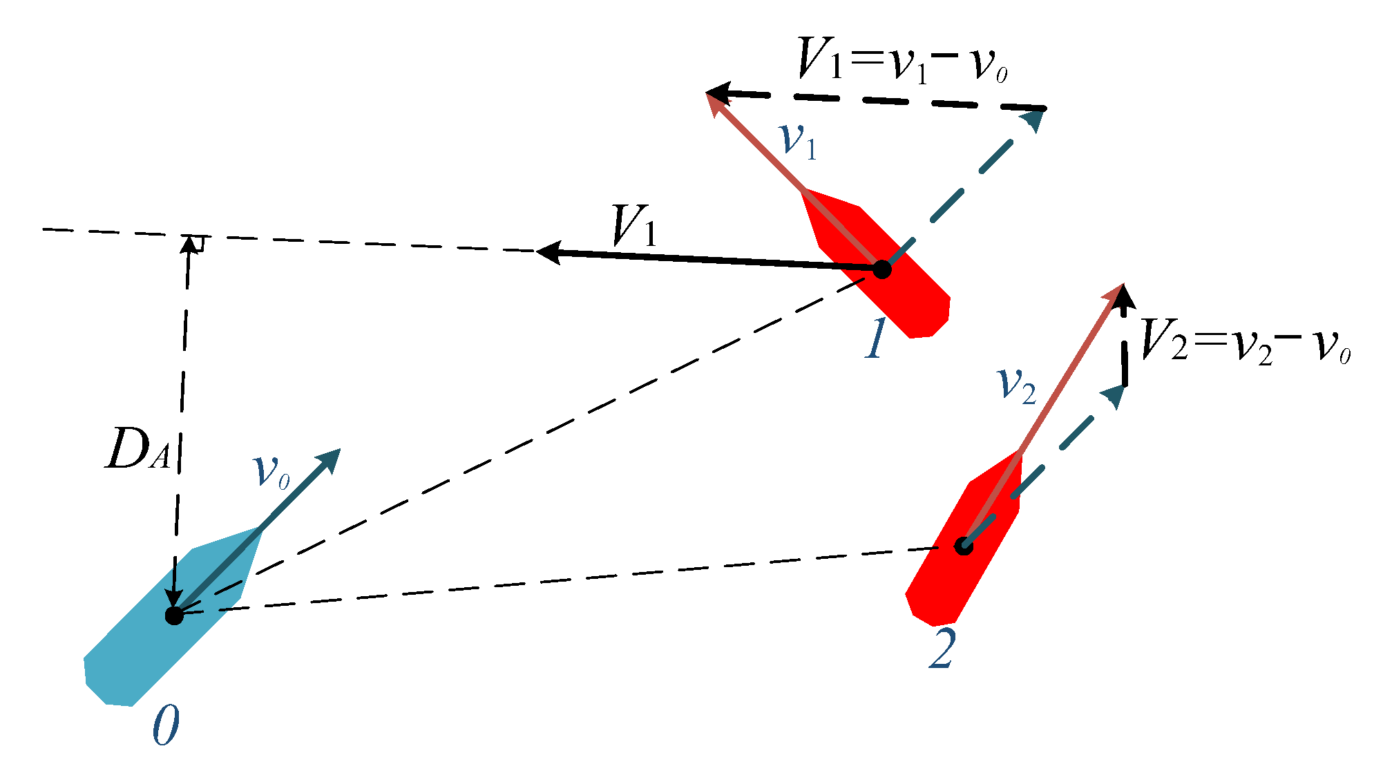
When evaluating collision risks with obstacles, the vessel safety field and safety distance are commonly used as vital factors. Unlike static obstacles, dynamic obstacles call for the consideration of both the current safety field and safety distance, as well as the prediction of safety field and safety distance trends for future temporal dynamic obstacles. As illustrated in
Figure 1, assume our vessel is located at point O, and the obstructing vessel moves from point A to point B, decreasing the distance between the two vessels from
to
and altering the azimuth angle
between them.
The ship safety field is an area centered on the vessel’s center of gravity. Although various safety field models with different shapes and judgments are employed in ship safety research, the safety distance standard remains widely utilized in the navigation process. The selection of a ship safety field must consider numerous factors. Existing research that overemphasizes the form of the ship safety field may not be conducive to the practical application of domain models.
For computational convenience, this paper treats the safety field of ships and other obstacle ships as circles, as illustrated in
Figure 2.
P0 represents the center of gravity of our ship’s safety field circle, while
P1 denotes the center of gravity of other ships.
signifies the total length of ships contained within the circumcircle,
s0 and
s1 are the adequate safety margins for both ships. When selecting the safety margin, the position data of the own ship and other ships should be considered, as well as the increase in field range due to the proportional effect of the ship. The product of
and the set factor
indicates that the radii of the expanded circles for the ship and other obstacle ships are
R0 and
R1, respectively.
By treating the safety field of ships and other obstacle ships as circles, the proposed method simplifies calculations while still providing a reasonable safety margin for both ships. This approach enables efficient and effective collision avoidance, considering the position data of both the own ship and other ships in the navigation process.
Building upon this, the distance between the expanded boundaries of the ship and other obstacle ships is denoted as
Ds. This distance considers the maneuverability parameters of the ship and other ships, their respective speeds, relative speeds, hydrological conditions, and other factors. During the voyage, the distance is also related to the respective headings of the own ship and other ships. Different encounter situations necessitate varying
Dm values. The radius of the ship safety field established in this paper is the safety distance between the ship and other ships, expressed as follows:
The illustration of ship safety field is shown in
Figure 3.
It is worth noting that there is a distinct difference between the ship safety field calculated based on the own ship and the ship safety field calculated according to other obstacle ships. The of the other ship differs from ours. Factors contributing to this difference include vessel size and maneuverability.
The expression for the ship safety distance
is as follows:
where
is the sampling period;
is the absolute value of the speed at which the two ships approach each other;
is the safe distance in the current navigation environment;
is the safe distance in the current environment;
is the safe distance in the current waters;
and
are the adjustment coefficients of
and
, respectively. In practical computations, according to the type of vessel and its suitable navigational waters, the values of
and
typically range from 0.3 to 1.2 nautical miles. Moreover, the values of
and
are adjusted based on the current environment and waters.
In order to effectively avoid collisions during a ship’s navigation, it is essential to have a well-designed collision avoidance decision algorithm that considers various factors and stages of the collision development process. The stages include long distance without danger, collision risk, emergency situation, urgent danger, and final collision. These stages represent the process of the distance between the own ship and the obstacle ship developing from near to far.
The collision avoidance decision algorithm should be capable of taking the most appropriate action to best avoid a collision when other ships are not maneuvering in accordance with the COLREGs or if the two ships are in close proximity due to some other reason. The algorithm should also be able to determine when to initiate collision avoidance maneuvers, as initiating them too early or too late could negatively impact the ship’s navigation.
When analyzing risk situations, the influence of other factors must be considered, particularly the distance between our ship and other obstacle ships as a constraint.
Figure 4 elucidates that in compliance with the COLREGs, the most crucial aspect is the closest point of approach
between the obstacle ship and the own ship and the collision risk detection distance
, which represents the distance allowing the vessel to undertake collision avoidance measures upon identifying a collision risk situation.
In this paper,
is defined as the sum of the safety field radius
and the potential field influence range radius
. The value of
is determined by the maximum value of the product of
times the obstacle’s bulking circle radius and
, with
set at 0.4. This definition allows for a comprehensive assessment of collision risk, considering both the safety and the potential fields’ influence on the ship’s navigation.
In this context, is a proportional coefficient referred to as the obstacle distance influence factor, which adjusts the potential field’s influence range depending on the distance between the ship and the obstacle.
4. Path Planning Based on Optimized APF
During the navigation process, the ship can use the APF method to take appropriate collision avoidance actions according to the COLREGs. Once the risk of collision is eliminated, the ship can resume sailing on the planned route and continue towards its destination. The APF method can adapt to changing environmental conditions and the movements of other ships, making it a suitable choice for intelligent ship navigation systems.
4.1. Construction and Calculation of Attractive Potential Field
At present, in the artificial potential field algorithm, the potential energy equation of the destination’s attractive potential field is usually transformed into a standard parabolic equation;
is the attractive potential field;
is the distance between the ship and the goal;
is the equation of the resultant velocity of our ship and the goal.
where
is scale weight factor for location,
is speed factor,
is the current position of the ship,
is the current position of the goal,
is the current speed of the ship,
is the current speed of the goal. When the ship sails in the two-dimensional space on the sea surface, the attractive potential field that the ship experiences is non-negative. Only when the relative position
and relative velocity
of the ship and the target point are all 0, is the attractive potential field 0.
According to the attractive potential field equation
, the attractive forces of equation
can be obtained:
The attractive forces equation
can be rewritten as
where the attractive force
represents the magnitude of the location-based influence, while
denotes the position vector. Additionally,
signifies the magnitude of the velocity-based attractive force, ensuring that the ship’s speed aligns with the target endpoint’s speed in both magnitude and direction upon arrival.
exhibits a positive correlation with
, with the direction coinciding with the target point’s movement relative to the ship and
representing the unit vector in the direction of velocity.
4.2. Construction and Calculation of Repulsive Potential Field
When the relative position between the vessel and other ships falls within the collision risk detection threshold, our vessel should adhere to the COLREGs and implement collision avoidance measures to achieve dynamic and static obstacle avoidance. The equation for the repulsive potential field of dynamic obstacles
in complex waters is
where
represents the proportional coefficient of the repulsive potential field generated by the dynamic obstacle,
denotes the maximum relative position line angle, and
is the distance between the vessel and the goal.
The equation for the repulsive potential field of a static obstacle
in open water is
where
represents the proportional coefficient of the repulsive potential field generated by the obstacle.
When ship encounters a static obstacle, the repulsive potential field it experiences depends on the distance between the ship and the static obstacle. Unlike the traditional repulsive potential field model, this model introduces a smaller constant:
. In this paper,
is chosen as the product of
times the
of the ship as the radius.
where
is an adjustment factor with a value range from 1 to 3. Its value is determined by considering factors such as the maneuverability of our ship, the ship’s length, the accuracy of sensor data (particularly position and distance), and an appropriate safety margin. The circle with the ship’s position as its center and
as its radius represents an area where no obstacles are allowed to enter. If any obstacle enters this area, it is considered a collision accident, so this area is called the forbidden zone. Within this range, the repulsive potential field is large enough and bounded to prevent our ship from colliding with other obstacles.
The total repulsive potential field equation is
By calculating the negative gradient of the repulsive potential field function
with respect to position and velocity, the corresponding repulsive force function expression
can be derived:
The equation of the ship under the resultant force is
Considering the presence of multiple static obstacles and dynamic obstacle ships, the resulting expression for the repulsive force acting on our vessel is as follows:
where
represents the repulsive force exerted by the
i-th ship or obstacle on the vessel and n refers to the total number of obstacles and other ships encountered by the vessel.
4.3. Ant Colony Optimization Algorithm
In path planning, the quality of a route often depends on multiple factors, such as distance, safety, and time consumption, thus forming a multi-objective optimization problem. The ant colony algorithm is a nature-inspired heuristic algorithm, drawing inspiration from the path optimization behavior of ants in search of food and avoidance of obstacles [
26]. Utilizing the global search capability and parallelism of the ant colony algorithm, satisfactory solutions can be effectively found in multi-objective optimization problems.
Specifically regarding local optima, the search may stall or cycle infinitely among several singular points when a local optimum or singularity is encountered. However, the ant colony algorithm selects the next node to visit based on the roulette wheel selection method, rather than choosing directly according to the size of the probability [
27]. This method expands the search range, enabling the search to possibly escape local optima and find the global optimum. The application of the ant colony algorithm in a global optimization strategy not only effectively enhances search efficiency but also avoids becoming trapped in local optima.
At time
, ant
selects the direction of travel from point
to point
based on the calculation of the state transition probability. By calculating the transition probability
of the available paths adjacent to point
, the transition probability of moving to grid point
is determined using the roulette wheel selection rule:
where
is the set of available nodes for the ant’s next step,
is the node transition probability,
is the pheromone concentration on the path,
is the heuristic function,
is the pheromone concentration coefficient, and
is the heuristic function coefficient. The definition of the heuristic function
is
In the formula,
represents the Euclidean distance between node
and node
. The definition of
is
To prevent an abundance of pheromones from leading subsequent ants astray in their path selection, the information along the path will be updated using the following method after each generation of ants completes their search:
In the formula,
represents the pheromone evaporation coefficient, and
denotes the increment of pheromones between points
and
during the current iteration.
where
represents the predefined number of ants in the colony, and
refers to the pheromones released by ant
as it traverses the path. The definition of
is
represents the initial pheromone value; denotes the total length of the path traversed by ant .
In traditional ant colony algorithms, the initial distribution of pheromones in the environment is set to the same value, leading to a certain degree of blindness in the initial path search by ants. This affects the search efficiency of the algorithm and increases the search time. In this paper, an improved method for initial pheromone distribution is proposed. This method calculates the initial pheromone
amount based on the number of obstacles surrounding a node. The specific implementation is as follows:
In the formula, is an enhancement coefficient that can be determined based on the actual situation; is an obstacle avoidance coefficient; represents the complement symbol; and is the set of adjacent pixels for the current pixel position. The function can be used to calculate the proportion of free pixels among the eight adjacent pixels of the current pixel. When there are fewer obstacle pixels in the neighborhood of the pixel, the initial pheromone of the pixel is larger; otherwise, the initial pheromone is smaller. This guides ants to advance and avoid searching in areas with too many obstacles, thus accelerating the convergence speed of the algorithm.
4.4. Collision Avoidance and Path Planning Algorithm Design
The method proposed in this paper first extracts key information from electronic chart data, such as ships, obstacles, and target points. The electronic chart is then converted into a rasterized image, where each grid cell represents either a navigable area or an obstacle. The system employs an ant colony algorithm for global path planning, initializing the ant population, heuristic information, and improved pheromone allocation, allowing ants to search and select the next grid cell on the rasterized image. Upon reaching the target point, the pheromone concentration is updated, the path length is recorded, and iterations are repeated, with the shortest path chosen as the global plan.
Local planning is achieved through an optimized artificial potential field method, calculating the attractive potential field (pointing towards the target) and repulsive potential field (moving away from obstacles) for static and dynamic obstacles. The composite potential field is obtained by combining these fields, which is used to calculate the ship’s moving direction. Dynamic obstacles are detected, and repulsive potential fields are applied, realizing local static and dynamic collision avoidance. The ship’s position is updated, and steps are repeated until the target is reached.
The global planning path of the ant colony algorithm and the local planning path of the optimized artificial potential field method are integrated to form the final ship path. The visualized final path is output for further analysis and use. Through this process, the combination of the optimized artificial potential field method and the ant colony algorithm is achieved, realizing ship path planning and dynamic collision avoidance in complex environments.
The traditional APF algorithm often encounters multiple local optima during the computation process. When it reaches these points, the search may stagnate or loop infinitely among several singular points, rendering the program unable to stop. Therefore, the search is likely to become trapped in these local optima, preventing it from finding the global optimum. To address this situation, this study proposes a fusion algorithm that incorporates an optimized ant colony algorithm to implement a global optimization strategy. The algorithm employs a roulette wheel selection method to choose the next node to visit, rather than making a direct choice based on the size of the probability. This approach broadens the search range, thereby locating the global optimum and avoiding becoming mired in local optima. For the optimization of the local planning APF method, a maximum number of iterations is set in this study. If the search exceeds this number without finding a satisfactory solution, the search is forcibly halted. The algorithm process proposed in this paper is illustrated in
Figure 5.
5. Results and Analysis
In this study, the traditional artificial potential field algorithm was optimized by considering ship types and parameters in the waters, as well as adhering to the requirements and specifications of the COLREGs. This enabled the establishment of a collision avoidance decision system for static and dynamic obstacles at sea and the realization of the ship’s autonomous obstacle avoidance decision and path-planning algorithm. To further validate the effectiveness, reliability, and real-time performance of the ship obstacle avoidance decision-making and path-planning algorithms based on the artificial potential field method, a simulation test of autonomous collision avoidance and navigation planning was conducted using the aforementioned ship autonomous collision avoidance system.
To meet real-world navigational task requirements, multiple simulation validations have been conducted in this study. Initially, tests for static avoidance and planning in three types of water areas, such as coastlines, islands, and reefs, were carried out to validate the performance of the proposed algorithm under varying static obstacles. Subsequently, tests were conducted under mixed dynamic and static obstacles to verify the algorithm’s stability and robustness under composite obstacle interference. Last, based on the COLREGs’ classification of vessel encounters, multiple encounter simulation tests were performed under different meeting patterns, simulating navigational situations in real waters. An in-depth discussion and analysis of the results followed the simulations.
In the simulation experiment, the positive direction of the vertical axis in the coordinate system represents north, while the positive direction of the horizontal axis represents east. The planned path of our ship is depicted by a blue trajectory, dynamic obstacle ships are represented by red dotted lines, and static obstacles are indicated by black color blocks.
5.1. Preprocessing of Electronic Nautical Chart Image Data
Prior to implementing the proposed algorithm, electronic nautical chart image data must undergo preprocessing. As shown in
Figure 6, this preprocessing includes image binarization and rasterization, which simplifies the data for subsequent simulation and validation. First, the electronic nautical chart image is binarized, converting elements, such as ships, obstacles, and target points, into black and white pixels to streamline the image information. Next, rasterization divides the electronic nautical chart into regular smaller areas, with each raster cell representing a navigable area or an obstacle. The raster cell size can be adjusted based on specific requirements and computational resources. In this study, the raster window value is set to five to reduce computation time without sacrificing accuracy.
This preprocessing method helps to simplify the geographical environment, providing clear and easily processed input data for the subsequent simulation and validation of the ant colony algorithm and the optimized artificial potential field method, thereby enhancing the efficiency and accuracy of path planning.
5.2. Static Obstacle Avoidance Simulation
In order to avoid collisions in restricted water areas, vessels need to consider different types of static obstacles. In this simulation experiment, an environment map corresponding to the electronic chart is established to accomplish autonomous ship obstacle avoidance decision-making and route-planning experiments. Analyses are conducted for coastlines, islands, and reefs, based on their specific characteristics.
- (1)
Coastline: The coastline, where land meets the sea, usually exhibits complex topography, possibly comprising beaches, cliffs, and bay currents. Coastal areas present a challenge for ship route planning due to the potential for shallow waters and complex terrain. Ships must maintain a certain distance to avoid grounding and collisions. Moreover, maritime currents and tidal factors in coastal areas must be factored into route planning, thus the repulsive potential field has a large range of influence;
- (2)
Islands: Islands are pieces of land in the sea, varying in size. The presence of islands may necessitate detours, especially in areas with many small islands, such as archipelagos or coral reefs. Concealed hazards, such as reefs and sandbars, may be present around some islands, posing higher demands for route planning;
- (3)
Reefs: Reefs are rocks or stones in the sea that can appear anywhere, including coastlines, around islands, and even in the open sea. Reefs pose a significant risk for ship route planning as they often lie below the water’s surface and are difficult to observe directly. If a ship strikes a reef, it may sustain severe damage or even sink. Therefore, safety and local optimization issues must be considered in ship route planning.
For ships navigating in restricted waters to avoid collisions, different types of static obstacles must be considered individually. In this section’s simulation experiment, obstacles are categorized into three types: coastlines, islands, and reefs, which are analyzed separately. The basic parameters of the subject vessel are presented in
Table 1.
Based on the electronic chart, a corresponding water environment map is created to carry out the ship’s autonomous collision avoidance decision-making and path-planning experiments.
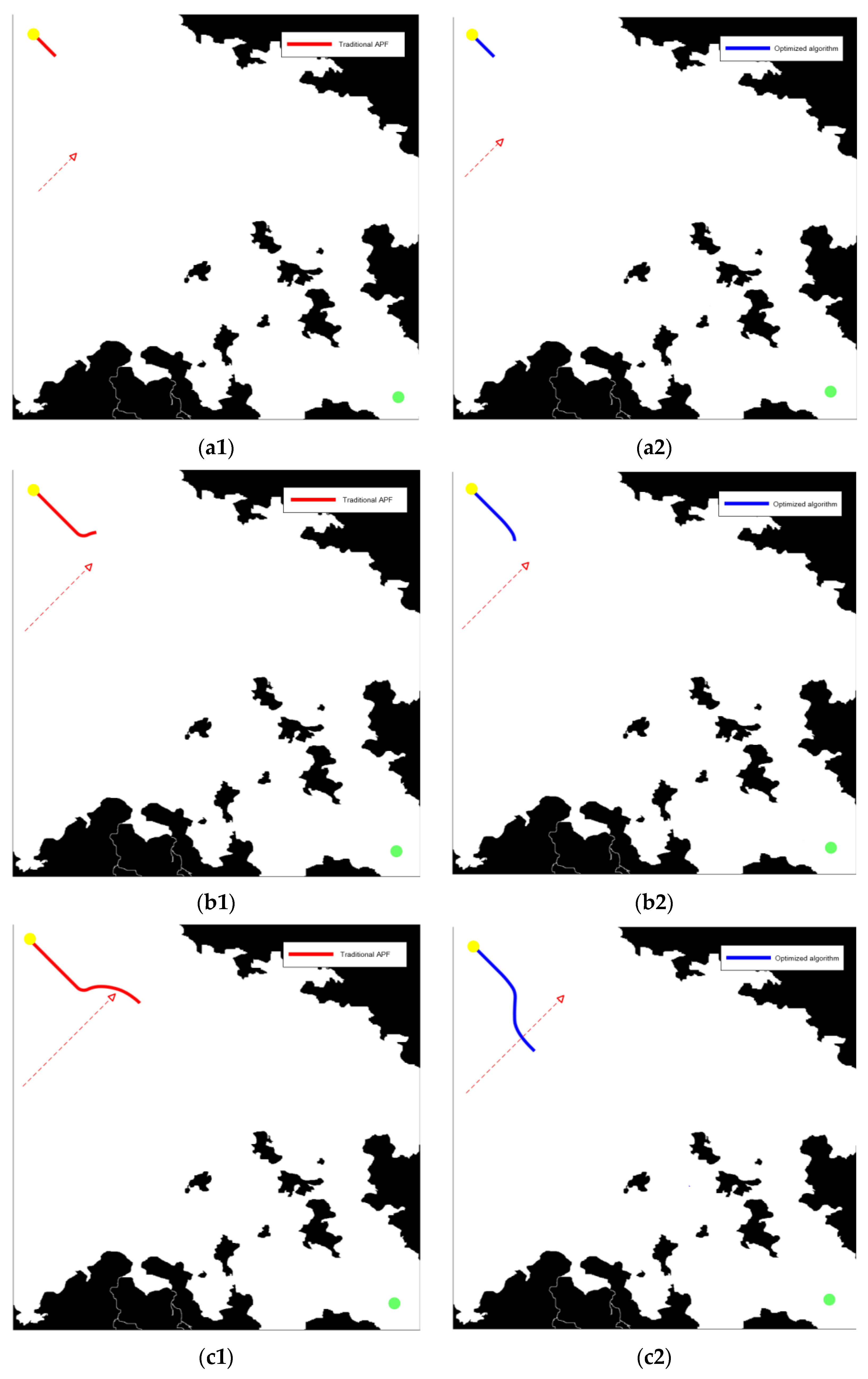
Simulation results are shown in
Figure 7, where black represents the projection of obstacles on the horizontal plane, and white areas indicate navigable regions for the ship. The simulation statistics are shown in
Table 2.
The simulation results presented in
Figure 7 and
Table 2 allow us to compare the trajectory planning of the traditional APF method and the optimized algorithm under three common marine environment obstacles. As can be seen clearly from
Figure 7a,b, the path of the optimized algorithm is shorter than that of the traditional APF method. By repeating this experiment 10 times, each result exhibits minor differences, demonstrating some randomness. The average path length is reduced by 17%, and the simulated curve is smoother.
Moreover, as shown in
Figure 7c, the traditional APF algorithm, under complex environmental conditions, stagnates due to the influence of multiple repulsive potential fields or becomes trapped in an infinite loop between several singular points, causing the program to become non-responsive. The path planning becomes stuck in these local optimal solutions, unable to find the global optimum. However, the optimized ant colony algorithm in this paper implements a global optimization strategy. It uses a roulette wheel selection method to choose the next node to be visited, instead of directly selecting according to the size of the probability. This strategy broadens the search range to find the global optimum and avoids falling into local optima, effectively resolving the local optimum problem present in the traditional APF method. However, due to the complexity of the optimized algorithm, the simulation computation time is longer than that of the traditional APF method, indicating a certain limitation.
5.3. Dynamic Obstacle Avoidance Simulation
Dynamic obstacle collision avoidance simulation refers to target ship navigating through and encountering obstacle ships, the parameters for the obstacle ship is delineated as depicted in
Table 3.
When the obstacle ship maintains its sailing state unchanged, our ship makes an emergency collision avoidance decision outside the safety domain. The starting position of my ship is designed, with an initial heading angle of −45° and a maximum speed of 16 knots. The obstacle ship has a sailing direction angle of 45° and maintains a speed of 10 knots. Under these circumstances, the simulation results of the proposed optimized algorithm are compared with the traditional dynamic APF method. The simulation results are illustrated in
Figure 8.
The simulation statistics are shown in
Table 4.
Analyzing the simulation results using the traditional dynamic artificial potential field method for collision avoidance simulations, the target vessel performs a 71° left turn when encountering a crossing situation with the obstacle vessel due to the lack of constraint from the vessel collision avoidance rule model, as shown in
Figure 8(b1). Furthermore, the distance between the target vessel and the obstacle ship is too small in
Figure 8(c1), and the vessel does not resume its course after avoiding the collision. These actions do not comply with COLREG requirements for vessel handling and safe navigation.
In contrast, as shown in
Figure 8(a2) and based on the optimized algorithm proposed in this paper, the target vessel detects an impending obstacle ship outside the safe zone. In
Figure 8(b2), it promptly takes evasive action and performs a collision avoidance maneuver by turning right 49°. This complies with COLREG requirements for vessel handling, adhering to the principle of turning right at an appropriate angle to yield and effectively clears the path in
Figure 8(c2). After completing the collision avoidance maneuver, the vessel resumes its course and eventually reaches its destination. During the path planning and collision avoidance process, the minimum distance between the target vessel and the obstacle ship is significantly greater than
+
, fulfilling the safety requirements for collision avoidance. After conducting this segment of the experiment five times, it is evident that the results of each trial vary slightly due to the stochastic roulette wheel structure of the ant colony algorithm. Despite the inherent randomness, the stability of the system remains unaffected. The average navigational distance is 18.84 n miles, with the greatest recorded distance being 19.30 n miles.
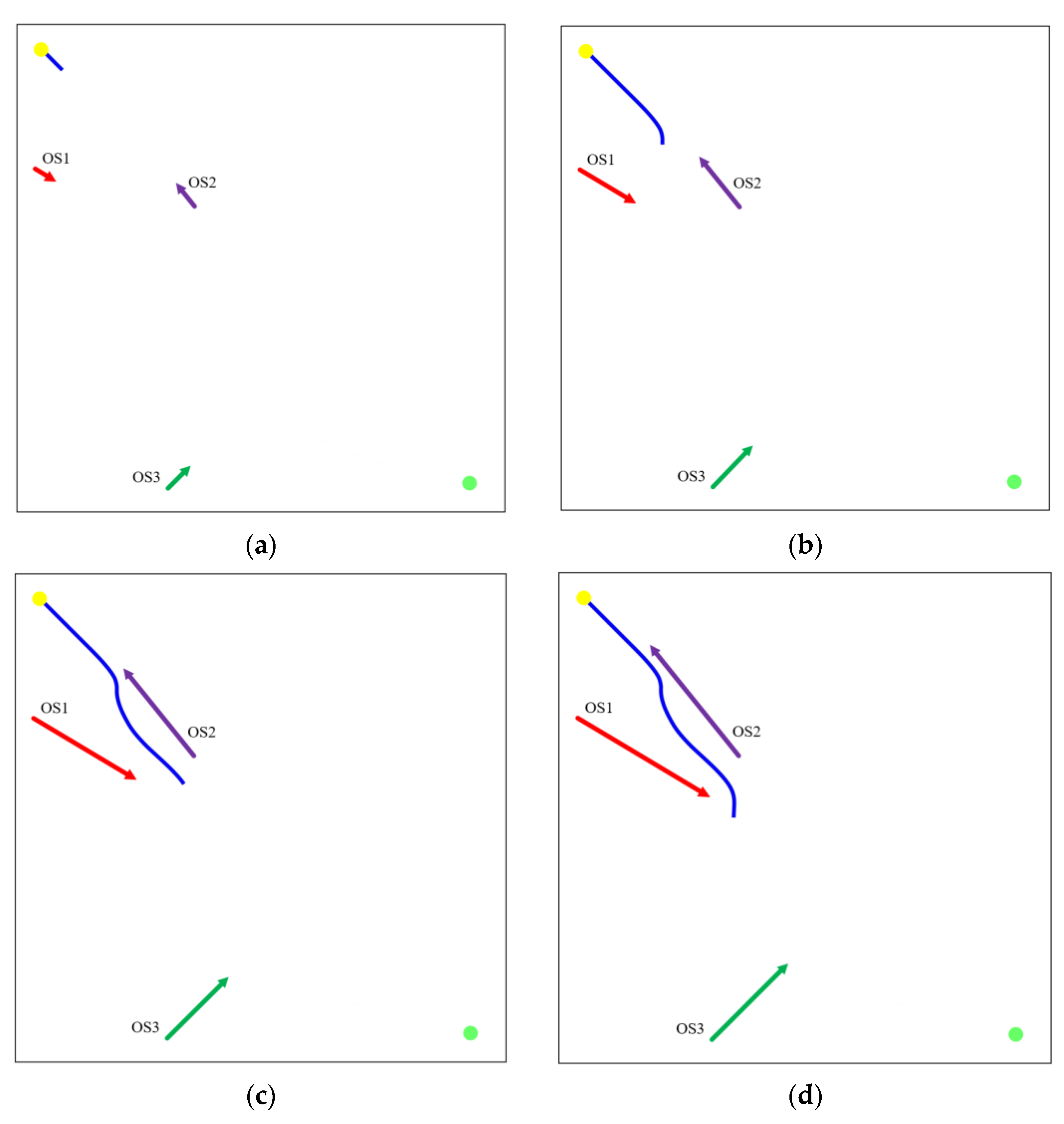
5.4. Validation of Multi-Ship and Multi-State Collision Avoidance
As per the COLREG ship encounter categorization, the encounters between the target ship and the obstacle ships are divided into three types: overtaking, head-on meeting, and crossing. This section will carry out multiple encounter simulation tests under different encounter modes, simulating the navigation situation in real waters. The parameters of the obstacle ships in the three typical meeting situations are shown in
Table 5.
The experiment is set in an open-water scenario, where three distinct obstructive vessels intersect the path of the target ship in different encounter scenarios.
Figure 9 demonstrates the result of the multi-vessel, multi-state collision avoidance test.
Based on the validation curves presented in
Figure 9, the statistical data garnered from simulation results, encompassing multiple vessels and diverse circumstantial collision avoidance, are articulated as exhibited in
Table 6.
According to the validation results in
Figure 9a, the target vessel has a course of −45° and is heading straight to the destination along the pre-planned route. Despite the presence of several obstructing vessels in this open sea, the distances between them are considerable and do not yet invade the safety distance criterion. Consequently, the target vessel is not within the influence range of the repulsive force field of the obstructing vessels and therefore does not take evasive actions.
Figure 9b shows that over time, both the target vessel and the obstructing vessel OS2 have traveled a certain distance, forming a head-on meeting situation. The target vessel enters the influence range of OS2’s repulsive field and makes a significant 42° right turn. The closest point of approach is 1.20 nautical miles, which meets the COLREGs and safety requirements, fully demonstrating the robustness and stability of the algorithm.
Figure 9c–e illustrate that after successfully avoiding OS2 with a right turn, the target vessel encounters a situation of overtaking OS1. Upon entering OS2’s repulsive field, the vessel makes a substantial 46° right turn following the algorithm’s constraints on vessel operations. The closest point of approach is 1.05 nautical miles. After evasion, the vessel resumes its course to the endpoint, meeting COLREG requirements.
Figure 9f–h demonstrate that after resuming its course, the target vessel intersects with the obstructing vessel OS3. The target vessel executes a substantial 53° right turn and passes from the rear side of OS3. The closest point of approach is 1.42 nautical miles. After completing the evasion, the vessel resumes its course and eventually reaches the endpoint.
Through the multi-vessel and multi-condition collision avoidance validation simulation, the algorithm’s capability to handle multiple meeting scenarios under COLREGs and multiple encounters in real waters is proven. The algorithm shows stability and robustness, and the evasive actions meet the normative requirements of the COLREGs.
In summary, the three sets of experiments validate the algorithm’s performance in static evasion and planning in restricted waters, collision avoidance under mixed static and dynamic obstacles, and collision avoidance in multiple encounters. The vessel’s evasive actions comply with regulations, and the planned route meets safety requirements. This indicates that the algorithm can prevent collisions in emergencies and that the planned route is a smooth curve, demonstrating its practicality.


