Effects of Inclination Angles on the Hydrodynamics of Knotless Net Panels in Currents

Abstract

Knotless nets have been extensively used in sea cages and offshore fish farms; the explicit illustrations of local flow patterns and subjected hydrodynamic loads have practical implications for the safe operations of aquaculture pens in open oceans. However, the effects of inclination angles of knotless nets on local flow patterns have not yet been fully discussed. In this paper, the effects of inclination angles on local time-averaged and instantaneous flow fields, velocity reductions and force coefficients are investigated using a $k-\omega$ shear stress transport-improved delayed detached eddy simulation (SST-IDDES) high-fidelity turbulence model. It is demonstrated that the inclination angles have dominant effects on the time-averaged velocity magnitudes around the net meshes. Secondly, the considerable flow interactions amongst the transverse and longitudinal net meshes, as well as cross-flow effects, are observed but weakened with the inclination angles. Thirdly, the profiles of velocity decelerations behind the net panels for 0${}^{\circ }$–45${}^{\circ }$ are not as trivial as those for 45${}^{\circ }$–90${}^{\circ }$. The associations between the embedded mechanism of subjected loads and pressure fields are established to analyse the current loads on nets in small inclination angles. The inclination angles are finally elaborated into the area-averaged velocity reduction and screen force models, then the improved characteristics are validated against the experimental data.

1. Introduction

The expanding progress of moving mariculture cages from coastal areas to open oceans is inevitable nowadays. Diverse from closed or semienclosed sites, offshore aquacultures are ordinarily located in fully exposed regions. It is well known that open oceans are substantially isolated from lands or islands, and combined with the harsh sea states, hint at the potential threat to the safety of aquaculture infrastructures. Rigid steel frames are utilised so as to form a constant cultural volume and shield the structures from extreme waves and currents, while flexible nets, are however justified, fragile enough that the subjected excessive hydrodynamic loads can induce fatigues or breakages of twines. Thus, the safety issues of nets in the excitation of energetic waves and currents are emphasised continuously in offshore fish farming. Knotless nets with square meshes have been widely utilised in deep-water sea cages and offshore aquaculture farms presently, for instance, braided nylon fabric nets (Figure 1a) and welded copper rigid nets (Figure 1b). The clarifications of flow distributions around nets, including time-averaged velocity properties, instantaneous turbulence fields and momentum reductions at the downstream vicinity, are theoretically and practically significant [1]. The predicted accuracies of subjected hydrodynamic loads, as well as the structural responses of sea cages, can be improved with a better knowledge of flow fields [2,3]. Further practical insights into flow fields are given as the correlations with fluid exchange rates and spreading patterns of nutrients across fish farms [4]. For example, the clarification of local flow fields can be used to assess the transportation of dissolved oxygen across net cages. Fish swimming behaviours are also closely associated with flow velocities inside cages. The design and operational guidelines of fishing nets or aquaculture farms require a better knowledge of hydrodynamic characteristics with various environmental scenarios and structural parameters. Practical implications, such as the improvement of trawl mouth expansions and the reduction in resistances of fishing gears, as well as biofouling, are closely concentrated with the hydrodynamic characteristics of nets. In summary, the flow around and wake behind nets, along with the subjected wave or current loads around nets, are of great significance for scientific research and engineering applications in aquaculture.

The hydrodynamic characteristics of nets in currents, including local flow distributions and induced loads, are ordinarily investigated through numerical methods and physical experiments. With regard to flow fields, Løland [5] derived the velocity attenuation patterns behind a 2D net panel theoretically and qualitatively. Taking wake-interacting features behind twines into consideration, the predicted formulae for velocity reductions behind a full-scale net panel were initially given. Cha et al. [6] obtained a near-field wake behind twines of chain-link woven copper alloy nets using particle image velocimetry (PIV) measurements, thereby confirming the significant effects of the unique structural shape and the weaving patterns on wakes. Bi et al. [7] analysed the flow velocity reductions behind fabric net panels with various net solidities using PIV and acoustic Doppler velocimetry (ADV), presenting the dominant relevance with net solidities and inclination angles. These findings keep in accordance with the numerical study by Endresen et al. [8] and the experimental test of knotless nets by Føre et al. [9]. The turbulence characteristics and mass transport in the near-wake region of the net panel are assessed through the PIV–planar laser-induced fluorescence (PIV-PLIF) method [10]; herein, the turbulent diffusivity is found to theoretically be in reasonable agreement with the Taylor diffusivity.

In addition to experimental techniques, numerical methods, including fluid–structure interaction (FSI) and computational fluid dynamics (CFD) methodologies, are also capable of analysing flow patterns. Patursson et al. [11], Bi et al. [12] and Yang et al. [13] studied downstream velocity reductions of fixed net panels through the equivalence of porous media, and the accuracies of the numerical method were validated against the published experimental data. Chen and Christensen [14] and Cheng et al. [15] incorporated porous media modelling with the lumped mass method and Morison force model, enabling a two-way coupling scheme and expanding its applicability to flexible nets and cages. Later, a novel coupling algorithm comprising the Lagrangian approach for net panels and the Eulerian fluid domain was proposed in Martin et al. [16], then flow reductions behind nets, cage-to-cage effects and full-scale net hydrodynamics in steel-frame fish farms [17,18] were reported. Inspired by cruciform configurations in net meshes [19], the Reynolds-averaged Navier-–Stokes (RANS)/large eddy simulation (LES) studies in Bi et al. [20], Zou et al. [21], Tang et al. [22] and Dutta et al. [23] were conducted to provide velocity profiles around cylinders, knots and cruciforms, then the impacts of mesh orientations, Reynolds numbers and so-called blockage ratios were also addressed. Benefiting from the advancements of computational abilities, a unique perspective for hydrodynamics opened up through the structural connections amongst circular cylinders, spheres, cruciforms and nets. Wang et al. [1] modelled net panels with 6 × 6 meshes using LES, then the distributions of turbulence kinetic energies and vorticity patterns over nets were firstly given. Furthermore, the lattice Boltzmann method was implemented and validated for the flow around net planes by Tu et al. [24]. The wake interactions behind planes were also justified through velocity profiles in this study, which are consistent with Løland [5] and Wang et al. [1].

On the other hand, the hydrodynamic loads on net panels are considerably correlated with materials, mesh shapes, structural parameters and biofouling, along with angles of attack (AOAs). In terms of metal net panels, Tsukrov et al. [25] and Cha et al. [6] measured hydrodynamic coefficients of woven, welded and chain-linked copper nets through water flume and PIV tests, respectively. Apart from solidity ratios and Reynolds numbers, the influences of weaving styles, surface roughness, knots and AOAs on the hydrodynamic coefficients of various metal nets were also discussed in detail. As for fabric nets, a comparative study between rectangular and cylindrical net panels was carried out to justify the close relevance of Reynolds numbers, solidities, inclinations and hydrodynamic loads [26]. With the same geometrical parameters, it was substantiated that the drag coefficient of a net bar is higher than a circular cylinder, and the drag coefficient of rectangular panels is also larger than that of cylindrical nets. Lader et al. [19] focused on the hydrodynamic properties of cruciform structures constituting net meshes, indicating that the sphere in a cruciform configuration can experience two to three times larger size than that without spheres. Following the concept of cylindrical cruciform elements forming nets, the drag coefficient of net panels was deduced from knots and twines, then the relevance of Reynolds numbers and solidity ratios were discussed through the experimental data [27]. For the long-term duration of aquaculture operations, the effects of biofouling were considered by Bi et al. [28], where it was found that accumulation can result in over 10 times larger loads on clean nets. With respect to net materials, hydrodynamic loads on the nylon and polyethylene net panels with twisted or knitted styles were examined through flume experiments [29,30], wherein the influences of monofilament or multifilament processing on the hydrodynamics were compared initially.

To the author’s best knowledge, the hydrodynamics of nets have been investigated for decades, whereas the effects of inclination angles of rigid and fabric nets on local flow patterns have not been fully discussed. Secondly, the embedded mechanism of subjected hydrodynamic loads has not been addressed by the flow distributions. Thirdly, Kristiansen and Faltinsen [31] proposed a novel screen-type force model predicting the hydrodynamic drags and lifts, represented by the Fourier series and bounded at the drag or lift coefficients of $\theta$ = 0${}^{\circ }$, 45${}^{\circ }$ and 90${}^{\circ }$. The predicted drag coefficient equals 0 for the $\theta$ = 90${}^{\circ }$, i.e., the incoming flow keeps parallel to the net panel. This estimation is, however, opposed to the physical observations of hydrodynamic drags of knotless net panels by Tang et al. [30] and Tang et al. [32], hinting at the downside of existing formulae.

Provided the adoption of high-fidelity CFD methods, it is feasible to introduce a wide range of inclination angles into the fitted formulae of the wake reduction model [1] and the screen-type force model [31], leading to further advancements in accuracies. In this research, the $k-\omega$ shear stress transport-improved delayed detached eddy simulation (SST-IDDES) turbulence model, enabling scale resolution at a lower computational cost than LES, was adopted to resolve the turbulence fields around net twines, while the far-field regions were modelled using RANS. The numerical framework, as well as the convergences of domains and grids, were successfully validated and justified in the author’s former published work [2]. The effects of the inclination angles of smooth rigid net panels on time-averaged and instantaneous flow fields, downstream momentum reductions and hydrodynamic coefficients were investigated in pure currents; the inclination angles were subsequently introduced into the wake reduction model and the screen force model. Finally, the updated screen force model was applied and validated in an FSI framework for simulating full-scale rigid and fabric nets in viscous fluids, including the approximations of subjected hydrodynamic loads and momentum reductions.

2. Numerical Modelling

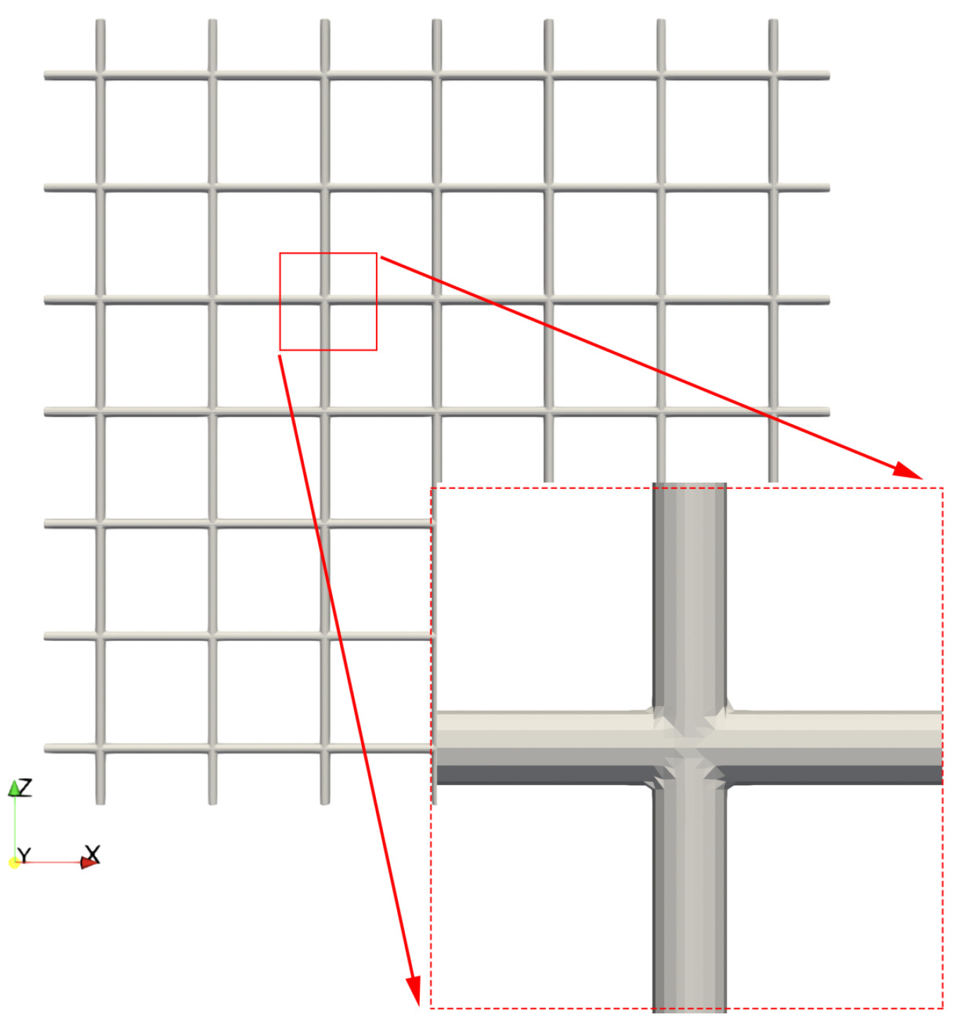
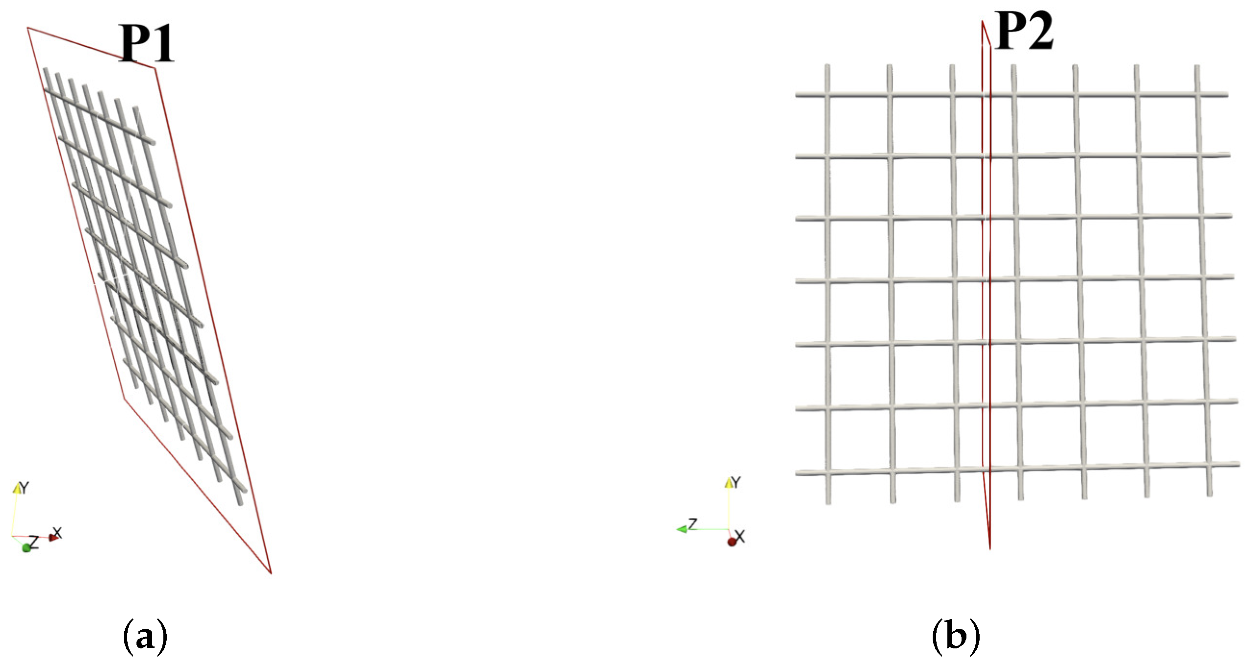
2.1. Net Panel Models

As revealed by Wang et al. [1,2] and Tang et al. [27], the dependencies of hydrodynamic behaviours with net solidities and Reynolds numbers are almost identical for rigid and fabric nets. The detailed weaving patterns of twines and knots cannot be accurately captured or modelled during numerical simulations, otherwise the accuracies can be sacrificed considerably. Thus, only smooth rigid knotless net panels with square meshes are used as the targeted models in CFD modellings (Figure 2). The investigated model scale was chosen as 6 × 6 meshes, achieving the mesh-number convergence of flow fields and drag force coefficients in the author’s published work [1]. Under the premise of saving computing resources, the high-resolution CFD simulation of small-scale net panels can reflect flow fields and hydrodynamic characteristics around full-scale nets to the greatest extent, while ignoring net deformations in currents.

The total of 65 computational cases were set to analyse the effects of inclination angles and structural and inflow properties on the hydrodynamic characteristics of net panels, as shown in

Table 1. The computational cases used in CFD simulations.

Cases	Incoming	Bar	Bar	Reynolds	Solidity
	Velocities	Diameters	Lengths	Number	Ratio
	${\mathit{U}}_0$ [m/s]	d [mm]	l [m]	$\mathbf{Re}$ [-]	${\mathit{S}}_{\mathit{n}}$ [-]
C1-0${}^{\circ }$, C1-22.5${}^{\circ }$, C1-45${}^{\circ }$, C1-67.5${}^{\circ }$, C1-90${}^{\circ }$	0.550	1.750	0.020	952.97	16.73%
C2-0${}^{\circ }$, C2-22.5${}^{\circ }$, C2-45${}^{\circ }$, C2-67.5${}^{\circ }$, C2-90${}^{\circ }$	0.100	1.750	0.020	172.97	16.73%
C3-0${}^{\circ }$, C3-22.5${}^{\circ }$, C3-45${}^{\circ }$, C3-67.5${}^{\circ }$, C3-90${}^{\circ }$	0.325	1.750	0.020	562.16	16.73%
C4-0${}^{\circ }$, C4-22.5${}^{\circ }$, C4-45${}^{\circ }$, C4-67.5${}^{\circ }$, C4-90${}^{\circ }$	0.775	1.750	0.020	1340.5	16.73%
C5-0${}^{\circ }$, C5-22.5${}^{\circ }$, C5-45${}^{\circ }$, C5-67.5${}^{\circ }$, C5-90${}^{\circ }$	1.000	1.750	0.020	1729.7	16.73%
C6-0${}^{\circ }$, C6-22.5${}^{\circ }$, C6-45${}^{\circ }$, C6-67.5${}^{\circ }$, C6-90${}^{\circ }$	0.550	0.500	0.020	326.44	4.940%
C7-0${}^{\circ }$, C7-22.5${}^{\circ }$, C7-45${}^{\circ }$, C7-67.5${}^{\circ }$, C7-90${}^{\circ }$	0.550	1.125	0.020	611.58	10.93%
C8-0${}^{\circ }$, C8-22.5${}^{\circ }$, C8-45${}^{\circ }$, C8-67.5${}^{\circ }$, C8-90${}^{\circ }$	0.550	2.375	0.020	1291.1	22.34%
C9-0${}^{\circ }$, C9-22.5${}^{\circ }$, C9-45${}^{\circ }$, C9-67.5${}^{\circ }$, C9-90${}^{\circ }$	0.550	3.000	0.020	1630.9	27.75%
C10-0${}^{\circ }$, C10-22.5${}^{\circ }$, C10-45${}^{\circ }$, C10-67.5${}^{\circ }$, C10-90${}^{\circ }$	0.550	1.750	0.010	951.35	31.94%
C11-0${}^{\circ }$, C11-22.5${}^{\circ }$, C11-45${}^{\circ }$, C11-67.5${}^{\circ }$, C11-90${}^{\circ }$	0.550	1.750	0.015	951.35	21.97%
C12-0${}^{\circ }$, C12-22.5${}^{\circ }$, C12-45${}^{\circ }$, C12-67.5${}^{\circ }$, C12-90${}^{\circ }$	0.550	1.750	0.025	951.35	13.51%
C13-0${}^{\circ }$, C13-22.5${}^{\circ }$, C13-45${}^{\circ }$, C13-67.5${}^{\circ }$, C13-90${}^{\circ }$	0.550	1.750	0.030	951.35	11.33%

. Following Føre et al. [9], the discrete sets of 0${}^{\circ }$, 22.5${}^{\circ }$, 45${}^{\circ }$, 67.5${}^{\circ }$ and 90${}^{\circ }$ were utilised to represent a broad scope of inclination angles. According to the marine fishery practice, the broadly adopted case C1 was selected to analyse the local flow properties, of which structural and inflow parameters were the medians across the investigated ranges. Concerning wake attenuation behind the net panels and subjected hydrodynamic loads, the structural parameters of the twines kept constant, while the integrated influences of incoming velocities $U_0$ and angles of attack $\theta$ were examined in cases C1–C5. C1, C6–C9 and C10–C13 were considered for the integrated effects of bar diameters d and bar lengths l, along with $\theta$, while keeping $U_0$ unaltered.

2.2. Viscous Fluid Dynamics Solver

$k-\omega$ SST-IDDES model was utilised to model the viscous fluids around the net panels and the wake behind them. As a hybrid methodology of RANS/LES for enabling a scale-resolving strategy, its original intention was to reduce the considerable computational cost of LES modelling, that is, RANS is used to model Reynolds stress or turbulent kinetic energy on the wall and far-field, while the LES method is capable of resolving the Reynolds stress or turbulent kinetic energy for the large-scale eddy motions on the near-wall regions. In contrast with the strategy that adopts the RANS model globally [20,21], the turbulence disturbance at downstream wakes as well as the flow separations from near-field boundary layers of cylindrical twines can be detected more precisely. As the basis of the IDDES method, the three-dimensional continuity and Navier–Stokes (N-S) equations are written in the convective form as

$$\begin{array}{cc}\hfill \nabla ·\overrightarrow{U}& =0,\hfill \\ \hfill {\displaystyle \frac{\partial \overrightarrow{U}}{\partial t}}+\overrightarrow{U}·\nabla \overrightarrow{U}& =-\frac{1}{\rho }\nabla p+\nabla ·\left(\nu [\nabla \overrightarrow{U}+\nabla {\overrightarrow{U}}^T]\right)+\overrightarrow{g}.\hfill \end{array}$$

(1)

where $\overrightarrow{U}$ represents the velocity vector; $\nabla p$ and $\rho$ denote the pressure gradient and the density of viscous fluids, respectively; $\overrightarrow{g}$ is the gravitational acceleration vector.

In the RANS part, the eddy viscosity in the diffusion term was enclosed using $k-\omega$ SST turbulence model [33]. The improving characters at accuracies and efficiencies of simulating flow separations from cylinders were dominant against the standard $k-\omega$ model. As for the IDDES method, Gritskevich et al. [34] enhanced the performance of the existing $k-\omega$ SST delayed detached eddy simulation (DDES) model without sacrificing the turbulence resolving in the vicinity of flow separations. IDDES method is derived by replacing the RANS length scale of the turbulent kinetic energy k equation with the IDDES length scale, while keeping the specific dissipation rate $\omega$ unaltered. The governing equations of k and $\omega$ in the SST-IDDES model read as [35]

$$\begin{array}{cc}\hfill \frac{\partial \rho k}{\partial t}+\nabla ·(\rho \overrightarrow{U}k)& =\nabla ·[(\mu +{\sigma }_k{\mu }_t)\nabla k]+P_k-\rho \sqrt{k^3}/l_{IDDES}.\hfill \end{array}$$

(2)

$$\begin{array}{cc}\hfill \frac{\partial \rho \omega }{\partial t}+\nabla ·(\rho \overrightarrow{U}\omega )& =\nabla ·[(\mu +{\sigma }_{\omega }{\mu }_t)\nabla \omega ]+2(1-F_1)\rho {\sigma }_{\omega 2}\frac{\nabla k·\nabla \omega }{\omega }+\alpha \frac{\rho }{{\mu }_t}{P}_k-\beta \rho {\omega }^2.\hfill \end{array}$$

(3)

$$\begin{array}{cc}\hfill {\mu }_t& =\rho \frac{a_1·k}{max(a_1·\omega ,F_2·S)}.\hfill \end{array}$$

(4)

where $F_1$ and $F_2$ denote the SST blending functions, which read as follows:

$$\begin{array}{cc}\hfill F_1& =tanh\left(ar{g}_1^4\right).\hfill \end{array}$$

(5)

$$\begin{array}{cc}\hfill ar{g}_1& =min\left(max\left(\frac{\sqrt{k}}{C_{\mu }\omega d_w},\frac{500\nu }{d_w^2\omega }\right),\frac{4\rho {\sigma }_{\omega 2}k}{C{D}_{k\omega }{d}_w^2}\right).\hfill \end{array}$$

(6)

$$\begin{array}{cc}\hfill C{D}_{k\omega }& =max\left(2\rho {\sigma }_{\omega 2}\frac{\nabla k·\nabla \omega }{\omega },{10}^{-10}\right).\hfill \end{array}$$

(7)

$$\begin{array}{cc}\hfill F_2& =tanh\left(ar{g}_2^2\right).\hfill \end{array}$$

(8)

$$\begin{array}{cc}\hfill ar{g}_2& =max\left(\frac{2\sqrt{k}}{C_{\mu }\omega d_w},\frac{500\nu }{d_w^2\omega }\right).\hfill \end{array}$$

(9)

where $d_w$ represents the distance to the nearest wall. The turbulence production term $P_k$ and IDDES length scale in Equation (2) are given below:

$$\begin{array}{cc}\hfill P_k& =min({\mu }_t{S}^2,10C_{\mu }\rho k\omega )\hfill \end{array}$$

(10)

$$\begin{array}{cc}\hfill l_{IDDES}& ={\tilde{f}}_d·(1+f_e)·l_{RANS}+(1-{\tilde{f}}_d)·l_{LES}\hfill \end{array}$$

(11)

$$\begin{array}{cc}\hfill l_{RANS}& =\frac{\sqrt{k}}{C_{\mu }\omega }\hfill \end{array}$$

(12)

$$\begin{array}{cc}\hfill l_{LES}& =C_{DES}\Delta \hfill \end{array}$$

(13)

$$\begin{array}{cc}\hfill C_{DES}& =C_{DES1}·F_1+C_{DES2}·(1-F_1).\hfill \end{array}$$

(14)

where $C_{DES1}=0.78$, $C_{DES2}=0.61$ and $\Delta$ is described as

$$\begin{array}{c}\hfill \Delta =min\left\{0.15max[d_w,h_{\max }],h_{\max }\right\}.\end{array}$$

(15)

where $h_{\max }$ denotes the length scale of computational grids, equalling the maximum length of all grid edges. Moreover, the empiric blending function embedded in Equation (14) is defined as ${\tilde{f}}_d=\max \{(1-f_{dt}),f_b\}$. The detailed procedures for calculating $f_{dt}$, $f_b$ and $f_e$ can be found in the study by Gritskevich et al. [34].

All the cases were simulated using the open-source CFD toolbox OpenFOAM v1806. The fluid properties of CFD simulations are listed in

Table 2. The fluid properties of CFD simulations.

Items	Data
Fluid material	Water
Density	998.3
Kinematic viscosity	1.19 × 10${}^{-6}$
Temperature	15${}^{\circ }$

. The transient solver pisoFoam accounting for pressure–velocity decoupling was used to solve the N-S equation. Considering balancing accuracies and stabilities, the convective terms were spatially discretised by the second-order linear-upwind stabilised transport (LUST) scheme with low-level numerical dissipation. The diffusive terms were treated through the second-order central difference scheme, while the temporal term advancement was processed with the second-order backward scheme. The time steps $\Delta t$ within unsteady simulations were determined as 0.005 d/U${}_0$, keeping the Courant–Friedrichs–Lewy (CFL) condition fluctuating at around 0.3–0.5. The pressure gradient was solved with the generalised geometric–algebraic multigrid (GAMG) method, while the momentum equation was solved through the Gauss—Seidel algorithm with additional smoothing for improved convergence.

2.3. Computational Domain, Grids and Boundary Conditions

As depicted in Figure 3a, the computational domain was determined as 16.0 l × 14.4 l × 14.4 l (length × width × height). The coordinate origin coincides with the geometrical centre of net panels, placed at 1/3 of the length and in the middle of the width and height directions. The inclination angle in this paper is defined as the intersection angle between the net plane and the gravity direction, as shown in Figure 3b.

Verified by Wang et al. [2], this configuration ensures that the water flow can fully develop before reaching the panel, and minimises the irrelevant influence from side boundaries of the computational domain on the hydrodynamics of nets. The left boundary in the domain was specified as the inlet condition, following the isotropic initialisations of k and $\omega$. The right-side boundary was assumed as the zero-pressure outlet condition, where $U_0$, k and $\omega$ respect the zero-gradient Neumann boundary conditions. The top and side boundaries were appointed as symmetry planes, that is, the normal components of the velocity and the normal gradients of all other variables were zero. The bottom plane and the net twines were both assumed as non-slip walls, but only the turbulent viscosity close to the bottom surface was modelled by wall functions.

The computational grids were generated using SnappyHexMesh in OpenFOAM. Owing to the meshing difficulties around net twines and numerous cruciform substructures, the unstructured hexahedral body-fitted grids are more capable of preserving an acceptable grid quality. Overview of the computational grids around the C1 case with the $\theta$ = 22.5${}^{\circ }$ as well as three refinement zones close to net twines were also set to capture turbulence fluctuations around the structure. A total of 13–15 boundary layer grids attached to the near-field region were generated with the expansion rate 1.1, satisfying that the first layer is inside the laminar sublayer of the boundary layer, i.e., $y^{+}<1$. According to the grid independence tests of flow fields and hydrodynamic coefficients [1,2], it 2qs determined that the grid size in the far-field area was 3.80 mm, while the most refined grids in the boundary layer remained $1.01\times {10}^{-5}$ m. The resulting grids had 40–50 M points.

2.4. Data Analysis

The time-averaged drag coefficient $C_D$ and the root-mean-square lift coefficient $C_L$ [11] were utilised to analyse the hydrodynamic drags $F_D$ and lifts $F_L$ on net panels with the outline area A. They are written as follows:

$$\begin{array}{cc}\hfill C_D& ={\displaystyle \frac{2F_D}{\rho A{U}_0^2}}\hfill \end{array}$$

(16)

$$\begin{array}{cc}\hfill C_L& ={\displaystyle \frac{2F_L}{\rho A{U}_0^2}}.\hfill \end{array}$$

(17)

3. Results and Discussions

3.1. Effects of Inclination Angles on Local Flow around Net Panels

The influences of the inclination angles of net panels on local flow fields are illustrated through two slicing planes (P1 and P2) across the net panels in the normal and tangential directions (Figure 4). For case C1 normal to the incoming flow, the nondimensional mean velocity magnitudes ($\left|U\right|/U_0$) simulated by the IDDES method keep in agreement with the LES observations by Wang et al. [1] (Figure 5). For the other cases, the inclination angles have dominant effects on the time-averaged velocity magnitudes in the tangential plane across the net panel, and the extent is obviously more pronounced than twine diameters and lengths. More specifically, there are considerable flow interactions amongst the transverse and longitudinal net meshes for the net panel perpendicular to the incoming current. The interacting effects are nevertheless weakened with larger AOAs, with the areas of local flow acceleration zones around twines presenting a shrinking tendency, while the low-speed regions are of larger dominances gradually. Until the net plane and the incoming flow are in parallel, the central regions of net meshes are fully occupied with downstream wakes, of which velocity magnitudes close to knots and net bars are almost decreased to zero.

In comparison to slice P1, the turbulence intensities of the flow fields at slice P2 are more significant, because viscous fluids are separating from cylindrical twines, resulting in an unsteady vortex shedding phenomenon behind nets in slice P2. Thus, the necessity of analysing instantaneous vorticity results in slice P2 has been emphasised to obtain a higher resolution of flow patterns. The modulus fields of the nondimensional instantaneous vorticity ($\left|\omega \right|d/U_0$) at slice P2 of the net panels with $\theta$ = 0${}^{\circ }$, 45${}^{\circ }$ and 90${}^{\circ }$ are depicted in Figure 6. For the case with $\theta$ = 0${}^{\circ }$, it is demonstrated that the vortex street behind the twine at the net boundaries shifts towards the outer edge in a marginal manner (see the deviated angles $\delta$ in Figure 6). This has the implications that the flow patterns around nets show similar characteristics to those around bluff bodies, as well as the so-called cross-flow properties for the downstream wakes. The IDDES results have also been observed in the published numerical studies [1,24], in addition to theoretical deductions [5]. However, one should notice that the deviations of downstream streamlines towards outer edges are not prominent for the case with $\theta$ = 45${}^{\circ }$. It can be attributed that the longitudinal layout of twines caused by the increase in inclination angles weakens the cross-flow. When $\theta$ = 90${}^{\circ }$, that is, the net bars perpendicular to P2 are entirely maintained in a tandem and longitudinal configuration with a spacing of 11.4d, the vortex shedding cannot be seen, as in Figure 6c. Further comparisons were given by Mittal et al. [36] that the vortex separations behind the tandem cylinders are considerable at a mere 5.5d spacing. A possible explanation for the difference is that the flow interactions induced by twines and cruciforms in vicinities still affect local flow fields, even in the case of small inclination angles.

3.2. Effects of Inclination Angles on Velocity Reductions behind Net Panels

In Figure 7, the very far-field wake regions of flowing past net panels are analysed through the normalised time-averaged velocity modulus extracted at $x/d=20$ behind the net panel. The trivial influences from the outlet boundary are avoided, as stated by Wang et al. [1]. For the case with 0${}^{\circ }$–45${}^{\circ }$, the velocity around the mesh centre can restore the initial momentum, while the velocity reductions are primarily concentrated in the downstream area where twines are projected. Thus, the overall differences in velocity distributions are not significant. With regard to the case with $\theta$ = 45${}^{\circ }$, the majority of wake regions are concentrated at the bottom of contours. This is attributed to the fact that the bottom vicinities remain much closer to the net panel, forming a dominant negative pressure zone and implying considerable momentum reductions. For $\theta$ = 45${}^{\circ }$–90${}^{\circ }$, the velocity attenuation regions are more concentrated in the area where the panel is projected to $x/d=20$ in the incoming flow direction. This trend is also justified quantificationally in the physical measurement of velocity reductions behind a net panel by Patursson et al. [11]. Furthermore, the flow velocities around the mesh centre cannot be restored yet due to the intense momentum reduction. The discrepancies of distributing patterns of velocity contours for the cases with $\theta$ = 45${}^{\circ }$–90${}^{\circ }$ are more significant against the cases with $\theta$ = 0${}^{\circ }$–45${}^{\circ }$. Therefore, it is of great necessity to carry out the comparative discussions between the velocity decreasing patterns for $\theta$ = 45${}^{\circ }$–90${}^{\circ }$ and $\theta$ = 0${}^{\circ }$–45${}^{\circ }$ in further investigations.

Based on the flow field data using $k-\omega$ SST-IDDES method, the area-averaged velocity reduction (AAVR) model suggested by Wang et al. [1] is utilised to quantify the effects of inclination angles and other factors, such as $Re$ and $S_n$, on the momentum attenuation behind net panels. The definition of AAVR is written as

$$\begin{array}{c}\hfill \mathrm{AAVR}={\displaystyle \frac{{\int }_A{(\overline{U}/U_0)}_{\mathrm{cell}}\mathrm{d}A}{A}}.\end{array}$$

(18)

where A denotes the area of the net panel projected to the rear plane of $x/d=20$, ${(\overline{U}/U_0)}_{cell}$ represents the nondimensional mean velocities at the dA dominated by the targeted cell centre and vicinity. Thus, the velocity reduction is estimated by combining the weight of each computational cell. The estimation quality can be improved compared to the commonly applied velocity reduction factor, assuming a constant value at a certain point in wake regions. The AAVRs of net panels perpendicular to currents with $Re$ and $S_n$ were fitted in Wang et al. [1], then the velocity reduction estimated formulae for rigid smooth and fabric nets were proposed with the validations against experimental data. The results of the AAVRs of all cases in this paper are summarised in

Table 3. The variation in AAVR with the inclinations of net panels amongst C1–C13.

Cases	Angles of Attack $\mathit{\theta }$ [Degree]
	0${}^{\circ }$ (Wang et al. [1])	22.5${}^{\circ }$	45${}^{\circ }$	67.5${}^{\circ }$	90${}^{\circ }$
C1	0.943	0.942	0.940	0.903	0.757
C2	0.933	0.921	0.925	0.875	0.754
C3	0.941	0.935	0.938	0.895	0.755
C4	0.944	0.945	0.944	0.918	0.753
C5	0.944	0.943	0.943	0.914	0.748
C6	0.987	0.986	0.983	0.976	0.756
C7	0.968	0.966	0.965	0.945	0.740
C8	0.883	0.889	0.894	0.868	0.790
C9	0.915	0.917	0.919	0.879	0.726
C10	0.855	0.853	0.870	0.831	0.747
C11	0.916	0.920	0.921	0.885	0.734
C12	0.971	0.971	0.968	0.944	0.768
C13	0.960	0.960	0.957	0.930	0.745

. It can be concluded that the AAVRs across $\theta$ = 0${}^{\circ }$–45${}^{\circ }$ are below 5% with the suitable range of $Re$ and $S_n$; thus, referring to the AAVR-predicted formulae [1] for nets normal to currents is acceptable, which is in agreement with the varying patterns of velocity contours with AOA (Figure 7). In contrast, the AAVRs of the cases of $\theta$ = 45${}^{\circ }$–90${}^{\circ }$ rapidly reduce to approximately 0.75, indicating the necessity of performing the nonlinear fittings between AAVRs and inclination angles in this scope. On the basis of the data in Table 3, nonlinear fitting is accomplished using the downhill simplex method [37]. As a result, the mean absolute percentage error (MAPE) between the Fourier series fitted formulae and the data in Table 3 remains 1.74%.

$$\begin{array}{cc}\hfill & \mathrm{AAVR}=\left\{\begin{array}{c}\hfill {\mathrm{AAVR}}_{0^{\circ }},0^{\circ }\le \theta \le {45}^{\circ }\\ \hfill {\mathrm{AAVR}}_{0^{\circ }}·\left(0.202sin2\theta +0.798\right),& \hfill & \hfill {45}^{\circ }\le \theta \le {90}^{\circ }\end{array}\right.\hfill \\ \hfill & {{\mathrm{AAVR}}_{0^{\circ }}}_{,\mathrm{smooth}}=(9.1\times {10}^{-6})Re-0.533S_n+1.021,\hfill \\ \hfill & {{\mathrm{AAVR}}_{0^{\circ }}}_{,\mathrm{fabric}}=(6.8\times {10}^{-6})Re-0.539S_n+1.016,\hfill \\ \hfill & 172.973\le Re\le 1729.728,4.94\%\le S_n\le 31.94\%.\hfill \end{array}$$

(19)

On account of the lack of experimental data on velocity reductions behind welded rigid net panels with various inclination angles, only the validations of AAVR models for fabric net panels were executed. Bi et al. [7] measured the mean velocities at the central wake regions of net panels with $\theta$ = 0${}^{\circ }$–60${}^{\circ }$ so that the validations of the novel AAVR model could be conducted to show the improved features.

Table 4. The validation of the AAVR-fitted formula.

Validation	Incoming	Angles of Attack	AAVR	Experimental	Relative
Cases	Velocities ${\mathit{U}}_0$ [m/s]	$\mathit{\theta }$ [Degree]	[-]	Data [-]	Discrepancies (RD) [-]
The knotless polyethylene net panel with d = 2.600 mm, l = 0.020 m	0.113	0	0.887	0.909	−2.42%
		30	0.887	0.897	−1.11%
		45	0.887	0.888	−0.11%
		60	0.863	0.851	1.41%
	0.170	0	0.888	0.912	−2.63%
		30	0.888	0.848	4.72%
		45	0.888	0.882	0.68%
		60	0.864	0.840	2.86%
	0.226	0	0.889	0.913	−2.63%
		30	0.889	0.890	−0.11%
		45	0.889	0.873	1.83%
		60	0.865	0.829	4.34%

lists the validation results as well as the relative divergences $\frac{\mathrm{AAVR}-\mathrm{EXP}.}{\mathrm{EXP}.}$(%). It is demonstrated that the relative divergences are below 5% within $U_0\le 0.226$ m/s; hence, the predicted accuracies of the improved AAVR models are verified across the cases of a wider range of inclination angles.

3.3. Effects of Inclination Angles on Hydrodynamic Coefficients

As mentioned above, the accuracy of the simulated hydrodynamic coefficients of net panels deserves further advancements, especially at small AOAs. In order to improve the accuracies of existing models, the influences of wide-range inclination angles (0${}^{\circ }$–90${}^{\circ }$) on $C_D$ and $C_L$ were studied following the high-resolution $k-\omega$ SST-IDDES method. As shown in Figure 8, the distributions of simulated $C_D$ and $C_L$ with AOAs over all cases are compatible with the laws revealed by Kristiansen and Faltinsen [31]. Nevertheless, the $C_D$ and $C_L$ for the case with $\theta$ = 90${}^{\circ }$ can be obtained as 0.08 and 0, respectively. As opposed to the typical formulae in Kristiansen and Faltinsen [31], this has the implication that $C_D$ of the cases with small inclination angles cannot be overlooked. This statement can be examined through the time-averaged pressure in slice P1 around the net panel with $\theta$ = 90${}^{\circ }$ (Figure 9). The pressure jump over the twines contributes to the hydrodynamic drag, which can be identified as the significant connection between hydrodynamic forces and flow fields. The simulated $C_L$ remaining around 0 is substantiated due to the highly symmetrical features of nets in the direction of lifts.

With respect to the corrections of existing screen force models, the nonlinear fittings amongst $C_D$, $C_L$ and the inclination angles were accomplished using the downhill simplex method [37]. Then, the estimated hydrodynamic coefficient formulae of the novel screen force model (NSFM) were proposed based on the CFD data and bounded by $C_D$ and $C_L$ at $\theta =0^{\circ }$ and ${45}^{\circ }$, as

$$\begin{array}{cc}\hfill C_D& =\left\{\begin{array}{ccc}\hfill C_{D,0^{\circ }}·\left(0.942cos\theta -0.019cos3\theta +0.077cos5\theta \right),& \hfill & \hfill 0^{\circ }\le \theta <{45}^{\circ }\\ \hfill C_{D,{45}^{\circ }}·\left(-0.687sin\theta +0.337sin2\theta +1.149\right),& \hfill & \hfill {45}^{\circ }\le \theta \le {90}^{\circ }\end{array}\right.\hfill \end{array}$$

(20)

$$\begin{array}{cc}\hfill C_L& =\left\{\begin{array}{ccc}\hfill C_{L,{45}^{\circ }}·\left(sin2\theta +0.150sin4\theta \right),& \hfill & \hfill 0^{\circ }\le \theta \le {45}^{\circ }\\ \hfill C_{L,{45}^{\circ }}·\left(0.951sin2\theta \right),& \hfill & \hfill {45}^{\circ }<\theta \le {90}^{\circ }\end{array}\right.\hfill \end{array}$$

(21)

Herein, $C_{D,0^{\circ }}$, $C_{D,{45}^{\circ }}$ and $C_{L,{45}^{\circ }}$ for fabric nets were separately calculated using the polynomial-fitted and power-fitted formulae [2], as in Equation (22). The applicability and accuracies of the polynomial-fitted formula applied for $C_D$ as well as the power-fitted formula for $C_L$ were elaborated and justified in [2].

$$\begin{array}{ll}{C}_{D,0^{\circ }}& =a_1{U}_0+a_{2}d+a_{3}l+a_4{U}_{0}d+a_5{U}_{0}l+a_{6}dl+a_7{U}_0^2+a_8{d}^2+a_9{l}^2+a_{10},\\ C_{D,{45}^{\circ }}& =a_1{U}_0+a_{2}d+a_{3}l+a_4{U}_{0}d+a_5{U}_{0}l+a_{6}dl+a_7{U}_0^2+a_8{d}^2+a_9{l}^2+a_{10}{U}_0^3+\\ & a_{11}{l}^3+a_{12}{U}_{0}dl+a_{13}{U}_0{d}^2+a_{14}{U}_0{l}^2+a_{15}d{U}_0^2+a_{16}d{l}^2+a_{17}l{U}_0^2+a_{18}l{d}^2+\\ & a_{19}{d}^3+a_{20},\\ C_{L,{45}^{\circ }}& =a_1{S}_n^{a_2}\ast R{e}^{a_3}+a_4,\\ & (0.1\mathrm{m}/\mathrm{s}<U_0<1\mathrm{m}/\mathrm{s},0.5\mathrm{mm}<d<3\mathrm{mm},0.01\mathrm{m}<l<0.03\mathrm{m},\\ & 50<Re<2970,3.31\%<S_n<51.0\%)\end{array}$$

(22)

with the coefficients in

Table 5. Coefficients for the polynomial- and power-fitted formulae of $\overline{C_D}$ and $\overline{C_L}$ [2].

	${\mathit{C}}_{\mathit{D},0^{\circ }}$	${\mathit{C}}_{\mathit{D},{45}^{\circ }}$	${\mathit{C}}_{\mathit{L},{45}^{\circ }}$
$a_1$	−0.132	−0.123	1.208
$a_2$	340.797	205.486	1.404
$a_3$	−59.643	−40.789	−0.099
$a_4$	−9.129	−22.592	0.005
$a_5$	2.245	−10.21
$a_6$	−12473.957	−12828.831
$a_7$	0.063	0.297
$a_8$	27831.591	60436.89
$a_9$	1458.245	1787.102
$a_{10}$	0.619	−0.121
$a_{11}$		−24020.784
$a_{12}$		706.455
$a_{13}$		3775.06
$a_{14}$		253.464
$a_{15}$		−9.623
$a_{16}$		128457.65
$a_{17}$		−0.025
$a_{18}$		−21641.925
$a_{19}$		−9227634.55
$a_{20}$		0.368

:

It was suggested by Kristiansen and Faltinsen [31] to use two harmonics to characterise $C_D$ and $C_L$, but the goodness of nonlinear fitting is insufficient if truncated after two coefficients. Thus, one more harmonic was introduced by Martin et al. [16] and Yao et al. [38] to evaluate drags and lifts, respectively. As opposed to the previous patterns, the harmonics and constants were revised extensively in the newly proposed formulae (Equations (20) and (21)) and truncated by $C_{D,0^{\circ }}$, $C_{D,{45}^{\circ }}$ and $C_{L,{45}^{\circ }}$. The divided-format function bounded by 45${}^{\circ }$ was also established simultaneously to fit the simulated data better, resulting in the MAPEs of $C_D$ and $C_L$ achieving 4.74% and 7.01% separately. It can be seen from Figure 8 that the fitting curves captured the majority of simulated data; thus, the effectivenesses of the nonlinear fittings were demonstrated from both qualitative and quantitative perspectives.

4. Applications and Validations of the Novel Screen Force Model

The newly proposed formulae of the screen force model derived from 6 × 6 meshes were applied to the full-scale net hydrodynamics solver in a fluid–structure coupling framework. Then, the simulated hydrodynamic loads on and momentum loss behind the full-scale net panels were compared against the published experimental data, showing the improved character of the NSFM.

4.1. The Fluid–Structure Coupling Method

Following the concept raised by Martin et al. [16], the net panel can be characterised by Lagrangian points coupled in an Eulerian fluid domain, modelling the physical fluid–structure interaction through an alternative fulfilment of the boundary conditions at the interface. A source term ${\mathbf{F}}_{\mathbf{net}}$ was incorporated into the right-hand side of Equation (1), describing the rapid pressure jump across the net panel, whereby the momentum losses of viscous fluids due to the presence of nets were identified and then estimated, observing the momentum conservation law of fluids. As an instance in Figure 10, it should be noted that one of the essential hypotheses is that momentum losses are assumed to be distributed isotropically around nets regardless of the presence of twines and knots. The uniformly distributed Lagrangian points are required, then the distance between the two ambient points is correlated with the cell size of the surrounding Eulerian grid. This dramatically improves the computational efficiency without evaluating the net geometrical details. This strategy can be naturally joined with screen force models, and similar simplifications were also utilised in previous studies of fluid–structure interactions [11,12,14,15]. The isotropic kernel D around ${\mathbf{x}}_i$ was introduced to account for the ${\mathbf{F}}_{\mathbf{net}}$ and the dominated vicinity, which is depicted by two averaged split triangles of one computational cell. Each split triangle is related to a specified Lagrangian point ${\mathbf{x}}_L$. Implemented in the open-source CFD toolbox REEF3D, the detailed coupling procedure as well as the sketch of isotropic kernels can be found in the studies by Martin et al. [16] and Martin et al. [17]. In brief, ${\mathbf{F}}_{\mathbf{net}}$ is established by relating subjected external forces with the covered region, which can be written as

$$\begin{array}{cc}\hfill {\mathbf{F}}_{\mathbf{net}}\left({\mathbf{x}}_i\right)& =\sum _{L=1}^{L_i}{\displaystyle \frac{{\mathbf{f}}_{\mathbf{net}}\left({\mathbf{x}}_L\right)}{\Delta x\Delta y\Delta z}}\mathrm{D}\left({\displaystyle \frac{x_i-x_L}{\Delta x}}\right)\mathrm{D}\left({\displaystyle \frac{y_i-y_L}{\Delta y}}\right)\mathrm{D}\left({\displaystyle \frac{z_i-z_L}{\Delta z}}\right).\hfill \end{array}$$

(23)

where $L_i$ denotes the number of Lagrangian points in the dominated vicinity of the isotropic kernel D around ${\mathbf{x}}_i$ [39]:

$$\begin{array}{c}\hfill \mathrm{D}\left(r\right)=\left\{\begin{array}{cc}{\displaystyle \frac{1}{4}}\left(1+cos\left({\displaystyle \frac{\pi r}{2}}\right)\right)\hfill & ,\left|r\right|<2.0,\hfill \\ 0.0\hfill & ,\left|r\right|\ge 2.0.\hfill \end{array}\right..\end{array}$$

(24)

For the fixed nets, the external forces at the Lagrangian point ${\mathbf{x}}_L$ dominated by the triangular screen element (with the area of $A_s$) are the integral of the hydrodynamic forces ${\mathbf{f}}_{\mathbf{h}}$, the gravity vector ${\mathbf{f}}_{\mathbf{g}}$ and the buoyancy ${\mathbf{f}}_{\mathbf{b}}$, as

$$\begin{array}{cc}\hfill {\mathbf{f}}_{\mathbf{net}}\left({\mathbf{x}}_L\right)& ={\left[{\mathbf{f}}_{\mathbf{h}}+{\mathbf{f}}_{\mathbf{g}}+{\mathbf{f}}_{\mathbf{b}}\right]}_L.\hfill \\ \hfill {\mathbf{f}}_{\mathbf{h}}& ={\displaystyle \frac{\rho }{2}}{A}_s{\mathbf{u}}_0^2(C_D{\mathbf{n}}_{\mathbf{d}}+C_L{\mathbf{n}}_{\mathbf{l}}).\hfill \end{array}$$

(25)

4.2. Validations of Hydrodynamic Forces on and Velocity Reductions behind Fixed Net Panels

In this section, the accuracy of subjected current forces as well as momentum loss behind fixed net panels are validated against the published experimental results. The original formulae within a classical screen force model (CSFM) derived by Kristiansen and Faltinsen [31] and refined by Martin et al. [16] are also utilised for further discussions. The net cases used in the validation part are illustrated in

Table 6. Overview of net cases used for the validation of the novel screen force model formulae.

Net Cases	AOA	${\mathit{U}}_0$	d	l	${\mathit{S}}_{\mathit{n}}$	References
	[degree]	[m/s]	[mm]	[cm]	[-]
N1	0	0.750	2.800	2.900	0.184	Patursson et al. [11]
N2	0	0.500
N3	0	0.125
N4	15	0.500
N5	30	0.500
N6	45	0.500
N7	60	0.500
N8	75	0.500
N9	0	0.500	1.450	1.300	0.211	Zhan et al. [26]
N10	30
N11	60
N12	22.5	1.000	2.000	1.730	0.230	Føre et al. [9]
N13	45
N14	67.5

. Three sets of experimental data from Patursson et al. [11], Zhan et al. [26] as well as Føre et al. [9] were adopted to examine the performance and applicability of NSFM for various net panels. In the study by Patursson et al. [11], the subjected drag/lift forces and downstream velocity losses of a 1 m × 1 m knotless nylon net panel with $S_n$ = 0.184 were measured in a 37 m (length) × 3.66 m (width) × 2.44 m (depth) towing tank, and the net panel was fixed with the rigid frame beneath the free surface of 0.732 m. The velocity reductions were observed at the centreline 2.5 m behind the net panel. A wide range of net inclination angles and free-stream velocities was considered, especially for the net case forming a small AOA (N8) with the free-stream direction. In contrast, the planar net panels used in Zhan et al. [26] were configured with square diamond meshes, towed in a 204 m (length) × 6 m (width) × 3 m (depth) tank. With regard to the experimental setup by Føre et al. [9], a larger net panel attached with the rigid frame of 1.215 × 0.985 m was utilised in a 10.5 m width and 5.6 m depth towing tank, and the evaluation point of the downstream velocities was located behind the net panel with a horizontal distance of 0.715 m. The lengths of numerical tanks across all net cases were reduced to improve computational efficiencies and discretised uniformly with a cell size of 0.05 m, based on the verification studies by Martin et al. [16].

The comparisons of the predicted hydrodynamic results by CSFM and NSFM against experimental measurements are illustrated in

Table 7. Validations of hydrodynamic coefficients (forces) and velocity reductions of net panels against experimental data.

Net Cases/	${\mathit{C}}_{\mathit{D}}$ [-]/${\mathit{F}}_{\mathit{D}}$ [N]			${\mathit{C}}_{\mathit{L}}$ [-]/${\mathit{F}}_{\mathit{L}}$ [N]			Velocity Reduction [-]
RD	Exp.	CSFM	NSFM	Exp.	CSFM	NSFM	Exp.	CSFM	NSFM
N1	0.257	0.298	0.243	-	-	-	0.100	0.137	0.111
		15.88%	−5.33%	-	-	-		36.19%	10.57%
N2	0.260	0.302	0.247	-	-	-	0.111	0.139	0.113
		16.24%	−5.12%	-	-	-		25.79%	2.26%
N3	0.266	0.324	0.265	-	-	-	0.074	0.041	0.047
		22.02%	−0.34%	-	-	-		−45.34%	−36.30%
N4	0.232	0.283	0.223	0.036	0.055	0.037	0.112	0.136	0.106
		22.38%	−3.50%		55.62%	3.37%		20.86%	−5.17%
N5	0.209	0.241	0.180	0.064	0.074	0.057	0.110	0.131	0.097
		15.73%	−13.67%		14.60%	−11.18%		19.45%	−11.51%
N6	0.157	0.192	0.152	0.066	0.068	0.056	0.114	0.127	0.101
		22.43%	−3.06%		3.05%	−13.89%		11.13%	−11.57%
N7	0.106	0.134	0.130	0.063	0.056	0.046	0.133	0.121	0.118
		25.80%	22.13%		−11.59%	−27.46%		−9.23%	−11.49%
N8	0.077	0.070	0.094	0.036	0.036	0.025	0.263	0.132	0.143
		−9.47%	22.31%		0.28%	−30.08%		−49.66%	−45.70%
N9	0.338	0.362	0.354	-	-	-	-	-	-
		7.20%	4.71%	-	-	-	-	-	-
N10	0.277	0.295	0.263	-	-	-	-	-	-
		6.49%	−5.01%	-	-	-	-	-	-
N11	0.165	0.163	0.165	-	-	-	-	-	-
		−1.75%	−0.30%	-	-	-	-	-	-
N12	171.429	194.388	163.586	36.735	51.144	35.339	-	-	-
		13.39%	−4.58%		39.23%	−3.80%	-	-	-
N13	123.324	140.011	118.609	45.481	48.797	39.390	-	-	-
		13.53%	−3.82%		7.29%	−13.39%	-	-	-
N14	80.467	73.797	82.551	29.738	34.440	25.194	-	-	-
		−8.29%	2.59%		15.81%	−15.28%	-	-	-

. As for hydrodynamic loads of N1–N3 with varying $U_0$, it can be seen that the NSFM performs better than CSFM with relative differences less than 6%. However, the velocity reduction of N3 with the minimum $U_0$ is underestimated substantially (36.30%), implying that the predicted ability of NSFM for the case with marginal turbulence fluctuations also needs further improvements. For N4–N8 with the larger inclinations, the hydrodynamic drags, lifts along with velocity losses are exhibited with more significant relative discrepancies between the NSFM and experimental results, but the NSFM in the majority of cases still performs overwhelmingly better than CSFM. The average error magnitude is 17.82% for the new formula versus 23.48% for the previous CSFM. A possible explanation was claimed by You et al. [40] that so-called dual effects, described as the various relationships between hydrodynamic parameters and net solidities with small inclination angles, are dominant for the larger discrepancies. For the cases by Zhan et al. [26] and Føre et al. [9], the improved properties of the NSFM formulae in estimating hydrodynamic drags were demonstrated with less than 5% deviation. In conclusion, the NSFM of hydrodynamic drags for the cases of $\theta \le {45}^{\circ }$ is justified, whereas the abilities for $\theta >{45}^{\circ }$ and the decelerations of fluid while passing net panels desire more advancements in terms of small AOAs.

5. Conclusions

In this paper, the effects of a wide range of inclination angles of knotless net panels on local time-averaged and instantaneous flow fields, momentum decelerations of fluids, and hydrodynamic force coefficients are comprehensively investigated using a $k-\omega$ shear stress transport-improved delayed detached eddy simulation (SST-IDDES) high-fidelity turbulence model. The conclusions are drawn as follows:

(1)

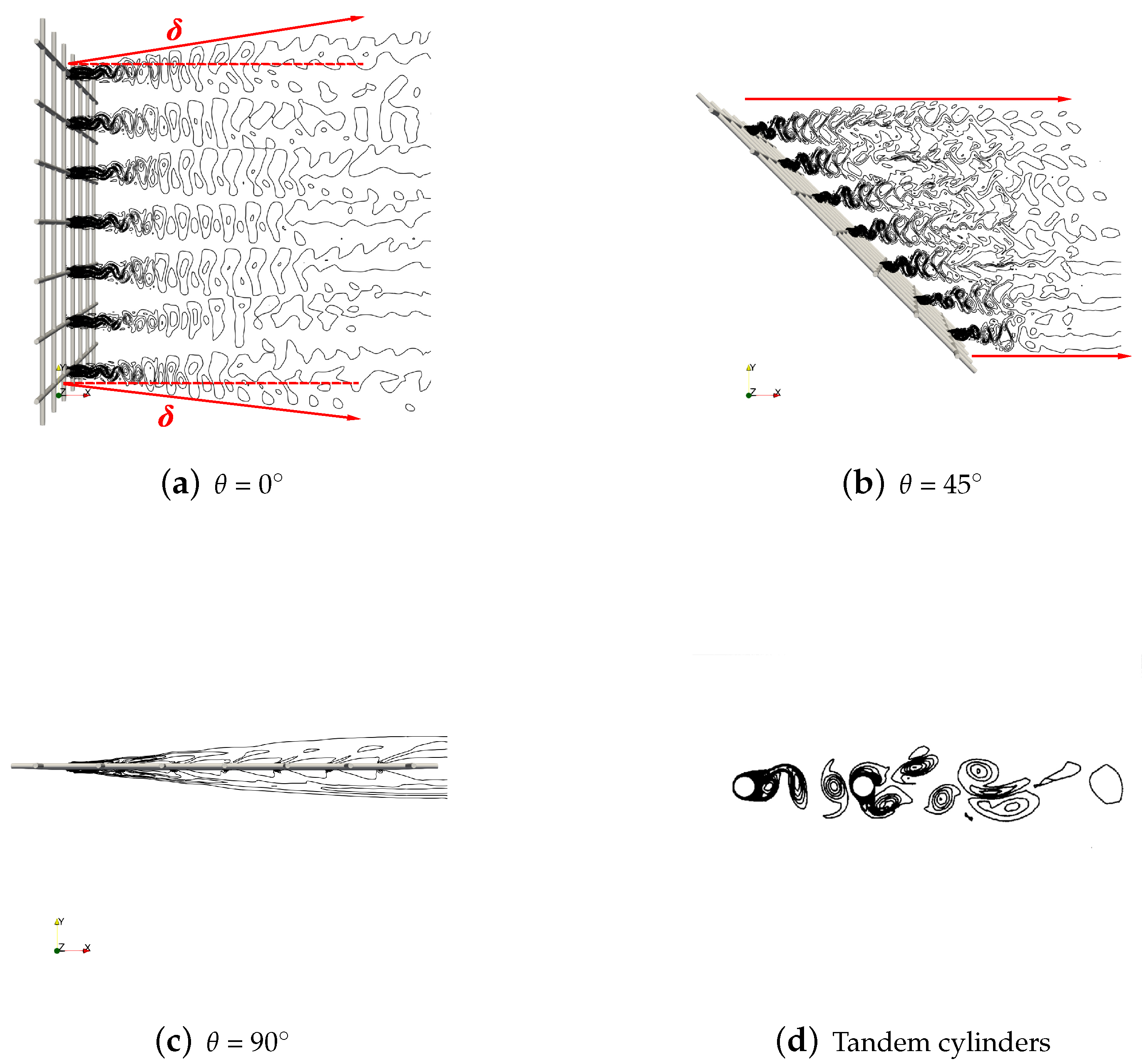
The inclination angles have dominant effects on the time-averaged velocity magnitudes around net meshes. More specifically, considerable flow interactions amongst the transverse and longitudinal net meshes for the net panel perpendicular to the incoming current are observed. The flow interacting effects amongst net meshes are nonetheless weakened at larger inclination angles. It can be seen that local flow acceleration zones around twines present a shrinking tendency, while low-speed regions are of larger dominance gradually.

(2)

From the transient vorticity fields, the so-called cross-flow properties at downstream wakes proposed by Løland [5] can be validated from our numerical results. Nevertheless, the longitudinal layout of twines induced by the increase in the inclination angles of nets has weakened the cross-flow properties.

(3)

The profiles of velocity decelerations behind the net panels for 0${}^{\circ }$–45${}^{\circ }$ are not as trivial as those for 45${}^{\circ }$–90${}^{\circ }$. For the case with 0${}^{\circ }$–45${}^{\circ }$, the velocity around the mesh centre can restore the initial momentum, while the velocity reductions are primarily concentrated in the downstream area where the twines are projected. Thus, the overall differences in velocity distributions are not significant. With regard to the case with $\theta$ = 45${}^{\circ }$–90${}^{\circ }$, the majority of wake regions are concentrated close to the bottom vicinities of contours.

(4)

Given the quantitative relationships between the downstream momentum losses and inclination angles, the novel formulae estimating downstream velocity reductions are further developed as an improvement of the former equations by Wang et al. [1]. The accuracies and applicabilities of the novel formulae with a broad scope of AOAs substantiate that the relative discrepancies of all validated cases are within 5% through the comparisons against experimental data.

(5)

The distributions of simulated $C_D$ and $C_L$ with inclination angles over all cases are compatible with the laws revealed by Kristiansen and Faltinsen [31]. Sensible differences can nevertheless be detected for the nets parallel to currents. This work has further elaborated Fourier-series formulae of screen force models, and the predicted hydrodynamics results by the improved and the previous formulae have been compared with the experimentally measured data. The improved features for hydrodynamic drags are justified, whereas the abilities for hydrodynamic lifts and the decelerations of fluid while passing net panels desire more advancements at small inclination angles.

References

1. Wang, G.; Martin, T.; Huang, L.; Bihs, H. Modelling the flow around and wake behind net panels using large eddy simulations. Ocean Eng. 2021, 239, 109846. [Google Scholar] [CrossRef]
2. Wang, G.; Martin, T.; Huang, L.; Bihs, H. An improved screen force model based on CFD simulations of the hydrodynamic loads on knotless net panels. Appl. Ocean Res. 2022, 118, 102965. [Google Scholar] [CrossRef]
3. Martin, T.; Bihs, H. A non-linear implicit approach for modelling the dynamics of porous tensile structures interacting with fluids. J. Fluids Struct. 2021, 100, 103168. [Google Scholar] [CrossRef]
4. Klebert, P.; Su, B. Turbulence and flow field alterations inside a fish sea cage and its wake. Appl. Ocean Res. 2020, 98, 102113. [Google Scholar] [CrossRef]
5. Løland, G. Current Forces on and Flow through Fish Farms. Ph.D. Thesis, Norwegian University of Science and Technology, Trondheim, Norway, 1991. [Google Scholar]
6. Cha, B.J.; Kim, H.Y.; Bae, J.H.; Yang, Y.S.; Kim, D.H. Analysis of the hydrodynamic characteristics of chain-link woven copper alloy nets for fish cages. Aquac. Eng. 2013, 56, 79–85. [Google Scholar] [CrossRef]
7. Bi, C.W.; Zhao, Y.P.; Dong, G.H.; Xu, T.J.; Gui, F.K. Experimental investigation of the reduction in flow velocity downstream from a fishing net. Aquac. Eng. 2013, 57, 71–81. [Google Scholar] [CrossRef]
8. Endresen, P.C.; Føre, M.; Fredheim, A.; Kristiansen, D.; Enerhaug, B. Numerical modeling of wake effect on aquaculture nets. In Proceedings of the ASME 2013 32nd International Conference on Ocean, Offshore and Arctic Engineering, Nantes, France, 9–14 June 2013. [Google Scholar] [CrossRef]
9. Føre, H.M.; Endresen, P.C.; Norvik, C.; Lader, P. Hydrodynamic Loads on Net Panels With Different Solidities. J. Offshore Mech. Arct. Eng. 2021, 143, 051901. [Google Scholar] [CrossRef]
10. Shao, D.; Huang, L.; Wang, R.Q.; Gualtieri, C.; Cuthbertson, A. Flow Turbulence Characteristics and Mass Transport in the Near Wake Region of an Aquaculture Cage Net Panel Flow Turbulence Characteristics and Mass Transport in the Near-Wake Region of an Aquaculture Cage Net Panel. Water 2021, 13, 294. [Google Scholar] [CrossRef]
11. Patursson, Ø.; Swift, M.R.; Tsukrov, I.; Simonsen, K.; Baldwin, K.; Fredriksson, D.W.; Celikkol, B. Development of a porous media model with application to flow through and around a net panel. Ocean Eng. 2010, 37, 314–324. [Google Scholar] [CrossRef]
12. Bi, C.W.; Zhao, Y.P.; Dong, G.H.; Xu, T.J.; Gui, F.K. Numerical simulation of the interaction between flow and flexible nets. J. Fluids Struct. 2014, 45, 180–201. [Google Scholar] [CrossRef]
13. Yang, X.; Zeng, X.; Gualtieri, C.; Cuthbertson, A.; Wang, R.Q.; Shao, D. Numerical Simulation of Scalar Mixing and Transport through a Fishing Net Panel. J. Mar. Sci. Eng. 2022, 10, 1511. [Google Scholar] [CrossRef]
14. Chen, H.; Christensen, E.D. Development of a numerical model for fluid-structure interaction analysis of flow through and around an aquaculture net cage. Ocean Eng. 2017, 142, 597–615. [Google Scholar] [CrossRef]
15. Cheng, H.; Chen, M.; Li, L.; Chen, H. Development of a coupling algorithm for fluid-structure interaction analysis of submerged aquaculture nets. Ocean Eng. 2022, 243, 110208. [Google Scholar] [CrossRef]
16. Martin, T.; Kamath, A.; Bihs, H. A Lagrangian approach for the coupled simulation of fixed net structures in a Eulerian fluid model. J. Fluids Struct. 2020, 94, 102962. [Google Scholar] [CrossRef]
17. Martin, T.; Tsarau, A.; Bihs, H. A numerical framework for modelling the dynamics of open ocean aquaculture structures in viscous fluids. Appl. Ocean Res. 2020, 106, 102410. [Google Scholar] [CrossRef]
18. Wang, G.; Martin, T.; Huang, L.; Bihs, H. Numerical investigation of the hydrodynamics of a submersible steel-frame offshore fish farm in regular waves using CFD. Ocean Eng. 2022, 256, 111528. [Google Scholar] [CrossRef]
19. Lader, P.; Enerhaug, B.; Fredheim, A.; Klebert, P.; Pettersen, B. Forces on a cruciform/sphere structure in uniform current. Ocean Eng. 2014, 82, 180–190. [Google Scholar] [CrossRef]
20. Bi, C.W.; Balash, C.; Matsubara, S.; Zhao, Y.P.; Dong, G.H. Effects of cylindrical cruciform patterns on fluid flow and drag as determined by CFD models. Ocean Eng. 2017, 135, 28–38. [Google Scholar] [CrossRef]
21. Zou, B.; Thierry, N.N.B.; Tang, H.; Xu, L.; Zhou, C.; Wang, X.; Dong, S.; Hu, F. Flow field and drag characteristics of netting of cruciform structures with various sizes of knot structure using CFD models. Appl. Ocean Res. 2020, 106, 102466. [Google Scholar] [CrossRef]
22. Tang, M.F.; Dong, G.H.; Xu, T.J.; Bi, C.w.; Wang, S. Large-eddy simulations of flow past cruciform circular cylinders in subcritical Reynolds numbers. Ocean Eng. 2021, 220, 108484. [Google Scholar] [CrossRef]
23. Dutta, D.; Bihs, H.; Afzal, M.S. Computational Fluid Dynamics modelling of hydrodynamic characteristics of oscillatory flow past a square cylinder using the level set method. Ocean Eng. 2022, 253, 111211. [Google Scholar] [CrossRef]
24. Tu, G.; Liu, H.; Ru, Z.; Shao, D.; Yang, W.; Sun, T.; Wang, H.; Gao, Y. Numerical analysis of the flows around fishing plane nets using the lattice Boltzmann method. Ocean Eng. 2020, 214, 107623. [Google Scholar] [CrossRef]
25. Tsukrov, I.; Drach, A.; Decew, J.; Robinson Swift, M.; Celikkol, B. Characterization of geometry and normal drag coefficients of copper nets. Ocean Eng. 2011, 38, 1979–1988. [Google Scholar] [CrossRef]
26. Zhan, J.M.; Jia, X.P.; Li, Y.S.; Sun, M.G.; Guo, G.X.; Hu, Y.Z. Analytical and experimental investigation of drag on nets of fish cages. Aquac. Eng. 2006, 35, 91–101. [Google Scholar] [CrossRef]
27. Tang, M.F.; Dong, G.H.; Xu, T.J.; Zhao, Y.P.; Bi, C.W.; Guo, W.J. Experimental analysis of the hydrodynamic coefficients of net panels in current. Appl. Ocean Res. 2018, 79, 253–261. [Google Scholar] [CrossRef]
28. Bi, C.W.; Zhao, Y.P.; Dong, G.H.; Wu, Z.M.; Zhang, Y.; Xu, T.J. Drag on and flow through the hydroid-fouled nets in currents. Ocean Eng. 2018, 161, 195–204. [Google Scholar] [CrossRef]
29. Zhou, C.; Xu, L.; Hu, F.; Qu, X. Hydrodynamic characteristics of knotless nylon netting normal to free stream and effect of inclination. Ocean Eng. 2015, 110, 89–97. [Google Scholar] [CrossRef]
30. Tang, H.; Hu, F.; Xu, L.; Dong, S.; Zhou, C.; Wang, X. The effect of netting solidity ratio and inclined angle on the hydrodynamic characteristics of knotless polyethylene netting. J. Ocean Univ. China 2017, 16, 814–822. [Google Scholar] [CrossRef]
31. Kristiansen, T.; Faltinsen, O.M. Modelling of current loads on aquaculture net cages. J. Fluids Struct. 2012, 34, 218–235. [Google Scholar] [CrossRef]
32. Tang, H.; Xu, L.; Hu, F. Hydrodynamic characteristics of knotted and knotless purse seine netting panels as determined in a flume tank. PLoS ONE 2018, 16, 814–822. [Google Scholar] [CrossRef]
33. Menter, F.R. Two-equation eddy-viscosity turbulence models for engineering applications. AIAA J. 1994, 32, 1598–1605. [Google Scholar] [CrossRef]
34. Gritskevich, M.S.; Garbaruk, A.V.; Schütze, J.; Menter, F.R. Development of DDES and IDDES formulations for the k-ω shear stress transport model. Flow Turbul. Combust. 2012, 88, 431–449. [Google Scholar] [CrossRef]
35. Menter, F.R.; Kuntz, M.; Langtry, R. Ten Years of Industrial Experience with the SST Turbulence Model. In Proceedings of the 4th International Symposium on Turbulence Heat and Mass Transfer, Antalya, Turkey, 12–17 October 2003; Volume 4, pp. 625–632. [Google Scholar]
36. Mittal, S.; Kumar, V.; Raghuvanshi, A. Unsteady incompressible flows past two cylinders in tandem and staggered arrangements. Int. J. Numer. Methods Fluids 1997, 25, 1315–1344. [Google Scholar] [CrossRef]
37. Nelder, J.A.; Mead, R. A simplex method for function minimization. Comput. J. 1965, 7, 308–313. [Google Scholar] [CrossRef]
38. Yao, Y.; Chen, Y.; Zhou, H.; Yang, H. Numerical modeling of current loads on a net cage considering fluid-structure interaction. J. Fluids Struct. 2016, 62, 350–366. [Google Scholar] [CrossRef]
39. Peskin, C.S. Numerical analysis of blood flow in the heart. J. Comput. Phys. 1977, 25, 220–252. [Google Scholar] [CrossRef]
40. You, X.; Hu, F.; Takahashi, Y.; Shiode, D.; Dong, S. Resistance performance and fluid-flow investigation of trawl plane netting at small angles of attack. Ocean Eng. 2021, 236, 109525. [Google Scholar] [CrossRef]
Figure 1. The illustrations of square-mesh nets with nylon fabric (a) and rigid copper (b) materials.
Jmse 11 01148 g001
Figure 2. The illustrations of the rigid net model with smooth surfaces.
Jmse 11 01148 g002
Figure 3. Overview of the computational domain, grids and angle of attacks.
Jmse 11 01148 g003
Figure 4. Definition of the sampling planes slicing through the net panel.
Jmse 11 01148 g004
Figure 5. The time-averaged nondimensional velocity magnitudes ( U / U 0 ) at slice P1 across net cases with varying inclinations.
Jmse 11 01148 g005
Figure 6. The instantaneous nondimensional vorticity fields ( ω d / U 0 ) at slice P2 across net cases with varying inclinations.
Jmse 11 01148 g006
Figure 7. The distributions of nondimensional mean velocity magnitudes at x / d = 20 behind the net panel.
Jmse 11 01148 g007
Figure 8. The distributions of the simulated hydrodynamic coefficients and the fitted curves.
Jmse 11 01148 g008
Figure 9. The mean normalised pressure contour around the net panel with θ = 90 .
Jmse 11 01148 g009
Figure 10. Overview of the full-scale net panel in pure currents using the FSI framework of REEF3D.
Jmse 11 01148 g010