Inland Vessel Travel Time Prediction via a Context-Aware Deep Learning Model

Abstract

Accurate vessel travel time estimation is crucial for optimizing port operations and ensuring port safety. Existing vessel travel time prediction models primarily rely on path-finding algorithms and corresponding distance/speed relationships to calculate travel time. However, these models overlook the complex nature of vessel travel time, which is influenced by multiple traffic-related factors such as collision avoidance, shortest path selection, and vessel personnel performance. The lack of consideration for these specific aspects limits the accuracy and applicability of current models. We propose a novel context-aware deep learning approach for inland vessel travel time prediction. Firstly, we introduce a complex network that captures vessel–vessel interaction contexts, providing valuable traffic environment information as an input for the deep learning model. Additionally, we employ a convolutional neural network to extract spatial trajectory information, which is then integrated with interaction contexts and indirect context information. In the vessel travel time prediction procedure, we utilize a long short-term memory network to capture the temporal dependence within consecutive channel sections’ fused multiple context feature sets. Extensive experiments incorporating historical data from the Wuhan section of the Yangtze River in China demonstrate the superiority of our proposed model over classical models in predicting vessel travel time. Importantly, our model accounts for the specific traffic contexts that had previously been overlooked, leading to improved accuracy and applicability in inland vessel travel time prediction.

1. Introduction

Maritime transportation accounts for the conveyance of over 80% of world trade cargo, rendering port resource scheduling a busy operation. Regarding port resources, berths provide parking spaces for vessels, and hoisting machines are the main pieces of equipment used for loading and unloading containers between container vessels and the front of a wharf. However, to ensure port safety and improve resource utilization efficiency, port managers must pre-allocate the different berths and hoisting machines depending on the sizes and types of arriving vessels (such as hazardous chemical vessels, container vessels, etc.). Therefore, the accurate estimation of vessel arrival time is crucial for optimizing port resources. Given that a vessel’s arrival time is a moment that is obtained by summing the vessel time T, a vessel travel’s time is vital to its arrival time. However, despite receiving estimated vessel travel time notifications 24 h in advance from port authorities, there can be discrepancies between the actual and reported vessel travel times due to various factors [1], including subjective factors such as the captain’s experience or environmental uncertainties leading to slowdowns. Therefore, the accurate prediction of vessel travel time is challenging and yet crucial for determining estimated time of arrival and supporting port resource scheduling.

An AIS (Automatic Identification System) is a system that actively transmits data from vessels regarding vessel movement information, such as longitude, latitude, speed, vessel type, time, maritime mobile service identity (MMSI), etc., through a transmitter. Hence, an AIS records useful information relative to travel time along the vessel’s itinerary, such as motion trajectory, regional vessel density, average speed, and the direct travel time from a fixed origin to the destination over time, making it beneficial for the prediction of vessel travel time.

While there appearssome growth in the research regarding travel time prediction based on AIS data, the amount of existing research is still limited. Wu investigated the problem of determining vessel travel times in inland channels; however, the focus in the cited study was identifying the distance from the origin to the destination and the corresponding timestamps based on an AIS [2]. More relevant research was presented in [3,4], where all of the developed travel time estimation algorithms follow a similar principle; that is, the travel time estimations are obtained by dividing an estimated path length by an estimated speed. For example, Alessandrini proposed an online path selection approach utilizing a grid structure network. This approach then employs the Dijkstra strategy to find the best next-step navigation grid based on the direction and density features of the current grid. The travel time to the destination is updated whenever a new grid is determined [3]. Park adopted reinforcement learning (RL) to predict paths and estimate average speed [4].

These studies mainly relied on the linear relationship between distance and speed, which may be invalid for long paths because longer paths may entail more uncertainties such as random deceleration. Considering the nonlinear relationship between multiple factors and travel time is a recent trend in related research. As a vessel’s navigation is affected by different route types and its personnel’s performance, Yu utilized machine learning models to determine the mapping relationship among vessel arrival times with respect to navigation day and month, route type, and vessel length [5]. Additionally, to account for the travel time difference in different motion patterns, Xu first employed a clustering algorithm to group motion patterns and then established travel time Support Vector Regression (SVR) models for each motion pattern, in which the inputs included the vessel’s latitude, longitude, speed over ground, course over ground, navigation status, and remaining distance and the output was the online travel time remaining until arriving at the destination [6].

However, few studies have explored the impact of traffic congestion information, which may impede a vessel’s motion on the surface. In areas with a high number of vessels, the average speed may decrease, thereby affecting travel time. In contrast, the prediction of travel time considering external factors is a well-researched topic in the road traffic literature, with many studies utilizing traffic flow and congestion to represent a traffic context.

For instance, Sheng used delay time to represent the congestion levels of road sections and constructed a convolutional long short-term neural network that fuses trajectory features and road traffic congestion information to predict travel times of different trajectories [7]. Peng constructed a time series relationship between travel time and traffic states, for which current and historical data were employed to predict the travel time of a given route in the next time interval [8]. Fei proposed a Bayesian dynamic linear model for real-time, short-term travel time prediction under two types of traffic statuses: recurrent and non-recurrent congestion [9]. Depicting the surface vessel congestion state and thus revealing the interactions between vessels is of great importance and as such deserves further study. Complex network theory has been applied in the aviation transportation domain to explain traffic congestion states [10]. It has also been applied in a maritime context to analyze conflicts between vessels, which will be utilized in our later work as traffic interaction information, where a high amount of conflict indicates a high level of congestion possibility, as reported in [11].

With the increasing prevalence of deep learning technology, there has been a growing interest in applying deep learning to determine the nonlinear mapping of multiple features in various domains. Kosarirad found that the sonar data generated by impellers with different numbers of blades had different typical characteristics. Therefore, he adopted multilayer perceptron neural networks to classify three types (three, four, and five blades, respectively) of vessel impeller sonar data [12]. The approach utilized high-dimension feature optimization and dimensionality reduction using a grasshopper algorithm to reduce the difficulty experienced by the model when attempting to learn nonlinear relationships and improve classification accuracy. In the road traffic domain, there are also some correlations that cannot be described or quantified by formulas, for example, the correlation between origin and destination. Sun proposed an LSTM network incorporating travel time information into the problem regarding the prediction of subsequent locations, finding that both location prediction and travel time actually improved next location prediction performance compared with only considering the last locations to predict future locations. The model revealed that travel time observations in a road may affect a driver’s location choices [13]. The powerful nonlinear fitting ability of deep learning gives us insights into establishing multi-source traffic information and determining vessels’ travel times.

In this paper, we propose a novel approach that utilizes deep learning models to effectively capture the correlation between multiple traffic context information and vessel travel time. Specifically, our proposed model employs a combination of CNN and LSTM networks to extract and analyze key features isolated from spatial trajectory data, ultimately providing insights into travel time estimation. The CNN plays a crucial role in capturing spatial trajectory features, while the LSTM network accounts for temporal dependencies in consecutive channel sections’ feature sets. By combining the strengths of CNN and LSTM networks, our proposed model effectively integrates spatial and temporal information to provide accurate and reliable travel time estimation. The model’s ability to extract and merge key features from vessel interactions, along with its capacity to capture temporal dependencies, allows it to discern intricate patterns and correlations that impact travel time.

The contributions of this work are as follows:

(1) We establish a Vessel Complex Interaction Network (VCIN) that reveals the surface traffic situation, wherein vessels are network nodes, and the interaction relationship corresponds to edges linking nodes. Compared to traditional traffic flow, the VCIN better describes the non-stationarity traffic context and implies more valuable information to predict travel time.

(2) We propose a vessel travel time prediction model based on three feature fusion modules: traffic context features, trajectory features, and environmental features. Spatial and temporal correlations are captured through convolutional processes and LSTM neural networks. The proposed model provides the opportunity to personalize vessel travel time recommendations based on a vessel’s power characteristics.

(3) We conduct a variety of comparison experiments using real data in the Wuhan section of the Yangtze River, China, which verify the potential causality between VCIN and travel time. Ablation experiments also demonstrate the advantage of our proposed model over state-of-the-art methods.

The remainder of the paper is organized as follows: Section 2 elaborates the multiple traffic information extraction procedure through three facets. Section 3 details the design of the vessel travel time prediction model. Section 4 presents the corresponding experimental prediction results and comparisons, utilizing the AIS data from the Wuhan section of the Yangtze River. Finally, Section 5 provides our concluding remarks.

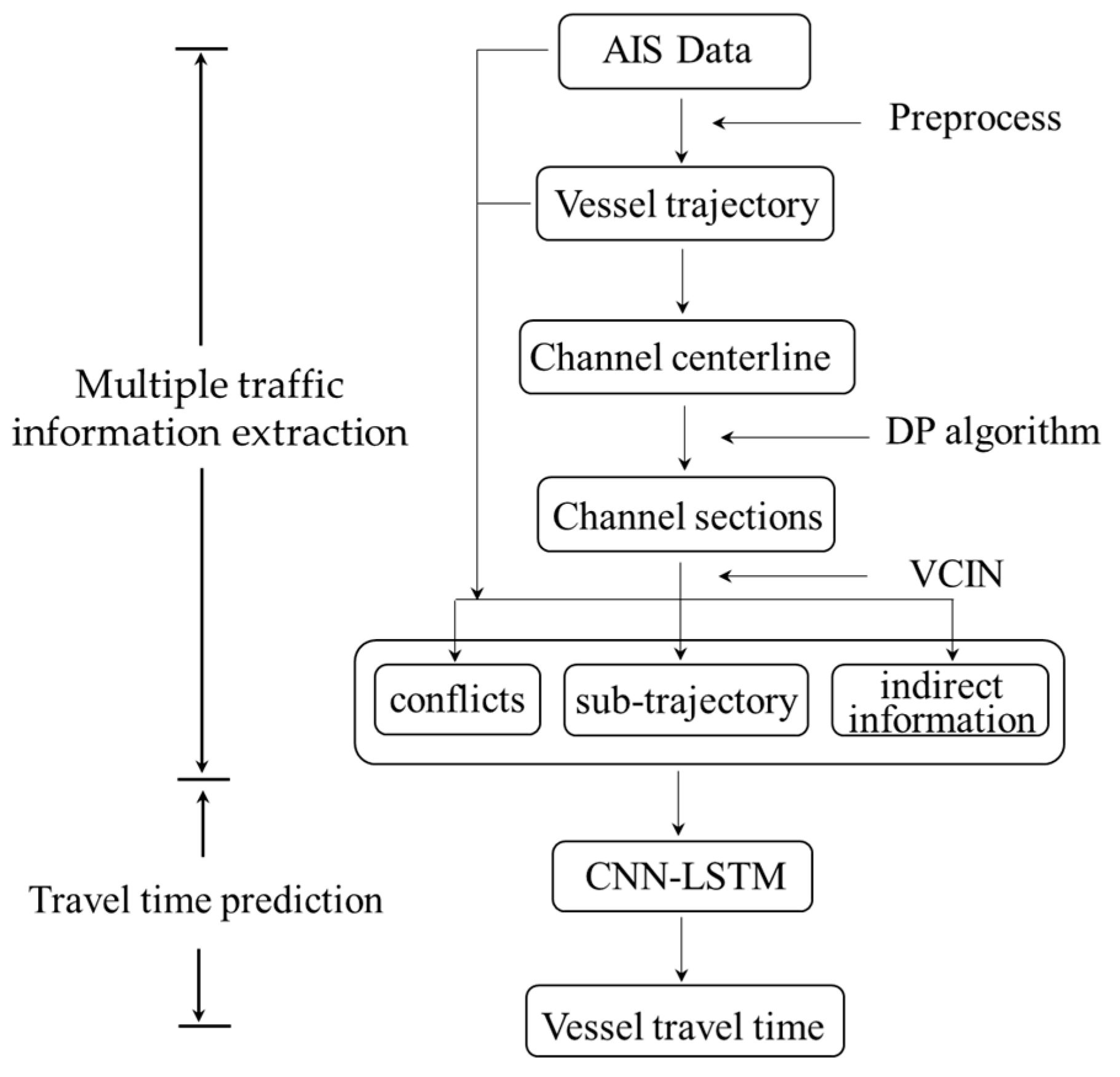
2. Multiple Traffic Information Extraction

The procedure of predicting inland vessel travel time mainly consists of two modules, as illustrated in Figure 1, including multiple traffic information extraction and travel time prediction. In Section 2, we clarify the first module with respect to two facets, namely, channel section division and sub-trajectory extraction, the traffic context extraction of sub-trajectory, where the Vessel Complex Interaction Network (VCIN) is proposed to depict the surface traffic context.

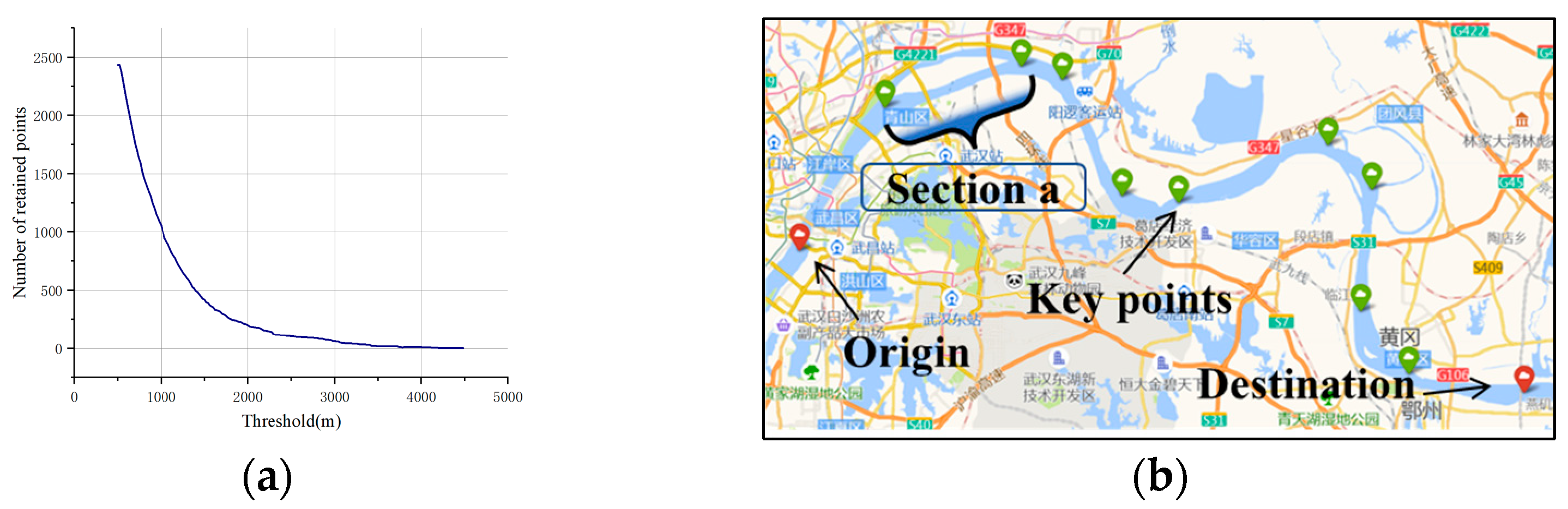
2.1. Channel Section Division and Sub-Trajectory Extraction

Trajectory information is a salient feature representing a vessel’s route; we decided to incorporate trajectory structure information into our deep learning model. However, incorporating the entirety of the trajectory may degrade model performance; thus, reducing the length of the trajectory can ease the model’s learning. For this reason, we first divided channel sections based on the Douglas and Peucker (DP) algorithm, and the sub-trajectories were formed according to keypoints falling into the corresponding channel sections.

We calculated the arithmetic mean of the upstream and downstream trajectories [14] to represent the channel centerline, which is shown in Figure 2.

Then, we employed the DP algorithm [15] to partition the channel centerline in order to detect the key points. Figure 2 illustrates the DP algorithm; it is typically a curve compression method used for the turning point detection of a curve through the identification of significant directional shifts. The algorithm searches for the farthest point p from the line defined by the first and last points. If the transverse distance $l$ to the line calculated using (1) exceeds the threshold, point p is saved, and the curve is then split at p to form a new line to which the algorithm is recursively applied. The solid line is the original curve connected by the collected points, and the dashed lines represent a DP simplified curve. As shown in Figure 2, $p_2$ is the first farthest point to the line defined by $p_0$ and $p_n$, and it is saved since the distance $l$ exceeds the threshold. However, since the distances $l_1$ and $l_3$ are both smaller than the threshold, the corresponding points $p_1$ and $p_3$ would be discarded

$$l=\frac{|{(y_b-y_a)}^{\mathrm{\ast }}{x}_p-(x_b-x_a{)}^{\mathrm{\ast }}{y}_p+x_b{y}_a-y_b{x}_a|}{\sqrt{{(x_b-x_a)}^2+{(y_b-y_a)}^2}}$$

(1)

where $l$ represents the distance from point $p$ to the line determined by $p_a=(x_a,y_a)$ and $p_b=(x_b,y_b)$.

The channel sections between each pair of retained points will be formed once the DP compression process is completed. We also determined the sub-trajectories, which are defined as the part of the vessel track that falls in a channel section. The sub-trajectory information is a salient feature representing the entire vessel route, wherein a longer sub-trajectory indicates a longer travel time. A CNN is then applied to extract the spatial structure of sub-trajectories, where the extracted information will combine with traffic context information to achieve prediction tasks.

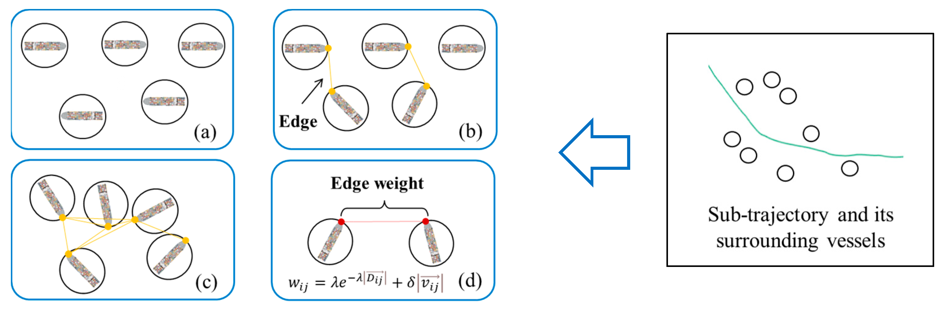
2.2. Traffic Context Extraction of Sub-Trajectory

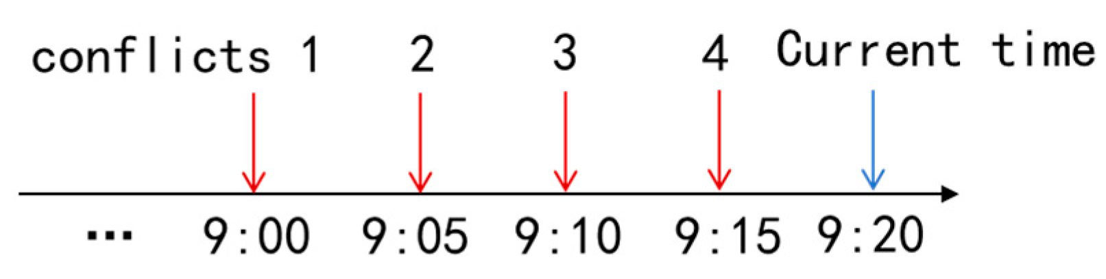
2.2.1. Interaction Information Extraction

Vessels may reduce their speed when facing an encounter [16], which, subsequently, may have an influence on the vessels’ travel time. Current algorithms are usually tested using vessel clusters or density to describe the traffic congestion. However, such methods only show the static features regarding the number of vessels in a region. Few studies consider the impact of the traffic interaction environment on the movement of vessels. In this section, we further incorporate the surface traffic dynamic interaction information into our deep learning model, which represents the environment congestion degree.

In a channel section, a vessel complex interaction network (VCIN) $G=\{V,E,W\}$ is defined as follows: $V=\left\{v_i\right|i\in I\}$ stands for the set of vessels, and $I=\{\mathrm{1,2},\dots ,N\}$, $E=\{e_{ij}=(v_i,v_j\left)\right|i,j\in I\}$ is the set of interaction links. N represents the number of regional vessels, and $W=\left\{w_{ij}\right|i,j\in I\}$ is the corresponding weight of $e_{ij}$. An example with five vessels is demonstrated in Figure 3.

The deduction of whether there is an interaction between a pair of vessels is determined by calculating their convergence and divergence relationships, which are represented by the approaching rate $R_{ij}$ in (2). If the approaching rate $R_{ij}$ is greater than or equal to 0, the vessel pair exhibits a divergence trend and does not have any interactions, as shown in Figure 3a. Otherwise, there is a convergence trend, indicating the possibility of congestion, as shown in Figure 3b,c; subsequently, the weight of each edge is calculated using Equation (3). The closer the relative distance and the greater the relative speed between vessels, the higher the risk of congestion or collision; therefore, we use the relative distance inverse function and relative speed to quantitatively express the weight in Equation (3)

$$R_{ij}=\frac{{\overrightarrow{D}}_{ij}\cdot {\overrightarrow{V}}_{ij}}{‖{\overrightarrow{D}}_{ij}‖}=‖{\overrightarrow{V}}_{ij}‖\cdot \mathrm{c}\mathrm{o}\mathrm{s} ({\overrightarrow{D}}_{ij},{\overrightarrow{V}}_{ij})$$

(2)

$$w_{ij}={\lambda e}^{-\lambda |{\overrightarrow{D}}_{ij}|}+\delta |{\overrightarrow{V}}_{ij}|$$

(3)

where ${\overrightarrow{D}}_{ij}$ and ${\overrightarrow{V}}_{ij}$ represent the vector distance and vector velocity of the two vessels, respectively. ${\overrightarrow{D}}_{ij}$ is calculated based on the two vessels’ coordinate information from an AIS, and ${\overrightarrow{V}}_{ij}$ is calculated based on speed information from the AIS. $\lambda$ and $\delta$ are coefficients that depend on the navigation environment.

The weight between each vessel pair presents a micro interaction situation. We sum all the weights in this channel section to account for the macro traffic interaction context, which is denoted as $conflicts$.

$$conflicts={\sum }_{i=1}^m{w}_{ij}$$

(4)

where m is the number of vessel pairs in a channel section whose $R_{ij}<0$.

To train the model, we extracted the sub-trajectory features in Section 2.1 and extracted four consecutive $conflicts$ values in the channel section corresponding to the sub-trajectory to represent the traffic context information, which was concatenated with the output of the convolution layer. That is, as shown in Figure 4, when the travel time prediction task is initiated at the current time of 9:20, four $conflicts$ values at 9:15, 9:10, 9:05, and 9:00 are extracted within a five-minute interval. These values are combined in the form of a vector.

2.2.2. Indirect Information Extraction

Indirect information such as date, vessel characteristics, and kinetic performance also influence a vessel’s travel time. For example, traffic flow exhibits short-term regular changes [5], with more vessels on the water during the day than at night. Additionally, long-term regularity, such as seasonal changes, and the kinetic performance of different vessels have an influence on vessel speed, leading to variations in travel time. Therefore, indirect information must be utilized to improve prediction accuracy.

However, it can be challenging for neural networks to disentangle the underlying meaning of text attributes. Inspired by previous work [17], we perform one-hot encoding for each categorical attribute, such as month, week, day/night, and vessel type, as shown in Figure 5. We then concatenate the resulting embeddings with the vessel’s digital information, such as vessel length, width, and power, resulting in a vector that can be used as an input to our deep learning model for prediction.

3. Vessel Travel Time Prediction Model

Multiple types of traffic information were extracted from Section 2.1 and Section 2.2 and used in the following sections. In this section, we present the results of deep learning techniques, specifically, CNN and LSTM networks, to extract spatial–temporal correlations between sub-trajectory and traffic context features to predict vessel travel time accurately. The framework of the travel time prediction model operating with multi-traffic information (TTP-MTI) is shown in Figure 6, where the inputs contain three aspects, namely, vessel sub-trajectory ($T$), traffic interaction context information ($conflicts$), and indirect information, and the output is the travel time consumed ($tt)$. The nonlinear relationship between them is shown in (5)

$$tt=f(T,conflicts,ind)$$

(5)

where $f$ represents the nonlinear function of the deep learning model.

Specifically, since the sub-trajectory feature best reflects the spatial evolution process of each vessel travelling, it is necessary to capture the feature of the sub-trajectory using a CNN. We use convolution layers to capture the spatial features with a 2D convolution kernel. The trajectory information after employing the CNN is mapped into a vector. The convolution layer is expressed as follows:

$${Con}_k=tanh(W_k\otimes T+b_k)$$

(6)

where ${Con}_k$ represents the $k\mathrm{th}$ characteristic of the convolution output. $tanh$ denotes the hyperbolic tangent activation function. $W_k$ stands for the weight matrix of the $k\mathrm{th}$ convolution kernel, and $b_k$ is the corresponding offset. $\otimes$ denotes convolution operation.

Then, we use the concatenate layer to fuse the sub-trajectory information, traffic interaction information, and indirect information to obtain the fused feature vector, as determined through (7). LSTM is adopted to memorize the long-term dependencies of a series of fused traffic data among consecutive channel sections, and the output is the travel time of the entire trajectory. It is worth mentioning that the ground truth of the travel time is obtained by manually subtracting the time from the origin and last trajectory point information (‘time’), which is used to calculate the loss of the model.

$${fused}_i=Con\oplus conflicts\oplus ind$$

(7)

$$tt=LSTM\{{fused}_1,{fused}_2 \dots ,{fused}_n\}$$

(8)

In the equation above, ${fused}_i$ represents the $i_{th}$ channel section fused information, $Con$ denotes $k$ convoluted features, and $\oplus$ indicates the concatenate operation.

In order to evaluate the prediction ability of our proposal model, we used three evaluation metrics—Root Mean Square Error (RMSE), Mean Absolute Error (MAE), and Mean Absolute Percentage Error (MAPE)—to calculate the difference between the prediction values and observations. RMSE is the most commonly used performance metric in traffic flow prediction research. The MAE is used to calculate the absolute error between the true travel time and the predictions, providing an intuitive measure of the error value. However, it cannot reflect the ratio of predictions relative to the original true value. Hence, we used the MAPE to calculate the ratio. Given that travel time is unlikely to have a true value of zero, the MAPE is a suitable index for prediction evaluation in our study.

$$\mathrm{R}\mathrm{M}\mathrm{S}\mathrm{E}=\sqrt{\frac{1}{n}{\sum }_{i=1}^n({\widehat{y}}_i-y_i{)}^2}$$

(9)

$$\mathrm{M}\mathrm{A}\mathrm{E}=\frac{1}{n}{\sum }_{i=1}^n‖{\widehat{y}}_i-y_i‖$$

(10)

$$\mathrm{M}\mathrm{A}\mathrm{P}\mathrm{E}=\frac{1}{n}{\sum }_{i=1}^n‖\frac{{\widehat{y}}_i-y_i}{y_i}‖$$

(11)

In the equation above, ${\widehat{y}}_i$ is the model-predicted vessel travel time value, while $y_i$ is the corresponding observation value.

4. Experiments

4.1. Resutls Regarding Channel Sections and Sub-Trajectries

The AIS data used in this paper were collected from the database of the Ship Supervision Center of the Wuhan Maritime Safety Administration, corresponding to a dataset covering an area of approximately 141 km in the Wuhan section of the Yangtze River and spanning 1 October to 1 December 2022, as shown in Figure 7. However, the AIS data as a series of messages following a nonstandard pattern of irregular time intervals and there are many bad datapoints due to transmitter failures, which often leads to inaccuracies or drift. Therefore, a preprocessing step was needed to clean the data and remove errors, which includes two aspects.

First, the AIS outliers concerning speed anomalies were eliminated based on the 3σ principle [18], the speed distribution and the fitted gauss curve are shown in Figure 3. Second, we manually eliminated bad AIS points with abnormal positions using the ArcGIS geographic information platform. Afterwards, we collected the normal AIS points for use in later research, as shown in Figure 8.

Each vessel has a unique MMSI and time information; therefore, we can obtain vessel trajectories according to each MMSI, and each trajectory is connected chronologically, as shown in Figure 9. It is worth noting that we only retained trajectories that did not include any intermediate stops or port stays as research objects, as this improved prediction accuracy. This is because we are only interested in determining the time it takes to travel through a section, regardless of any operational processes that occur at the port.

We created two separate datasets based on the trajectory course information: the Upstream and Downstream datasets. The Upstream dataset contains 2105 trajectories, while the Downstream dataset consists of 2165 trajectories. A total of 4270 vessel trajectories were selected for later research. Detailed vessel-type information is presented in

Table 1. Details of the data for training and testing.

Splitting Data	Trajectory Patterns
	Upstream	Downstream
Oil tanker	494	544
Cargo	302	471
Container	463	431
Chemical tanker	210	202
Multiple vessel	636	517
Total	2105	2165

.

The channel centerline was obtained by determining the arithmetic mean of the Upstream and Downstream trajectories. We applied DP to the channel centerline to retain the key points. The relationship between the threshold distance of the DP and the number of retained points of the channel centerline is depicted in Figure 10a. It can be observed that as the distance increases, the number of key points decreases and tends to stabilize. While we need to ensure adequate representations to build channel sections, we set the threshold distance to 3500 m in our study, which resulted in obtaining 11 key points along the Yangtze River from Wuhan to Ezhou. A visualization of the key points that form the channel sections is shown in Figure 10b.

The entire trajectories were segmented according to the key points, and we displayed part of vessel sub-trajectories, where each sub-trajectory is labeled with its vessel type, as shown in Figure 11. Inspired by previous work [7], the sub-trajectories were then projected onto two-dimensional pictures. A CNN was then applied to extract the spatial structure relationships between the vectors, where the extracted information was combined with traffic interaction information to predict vessel travel time.

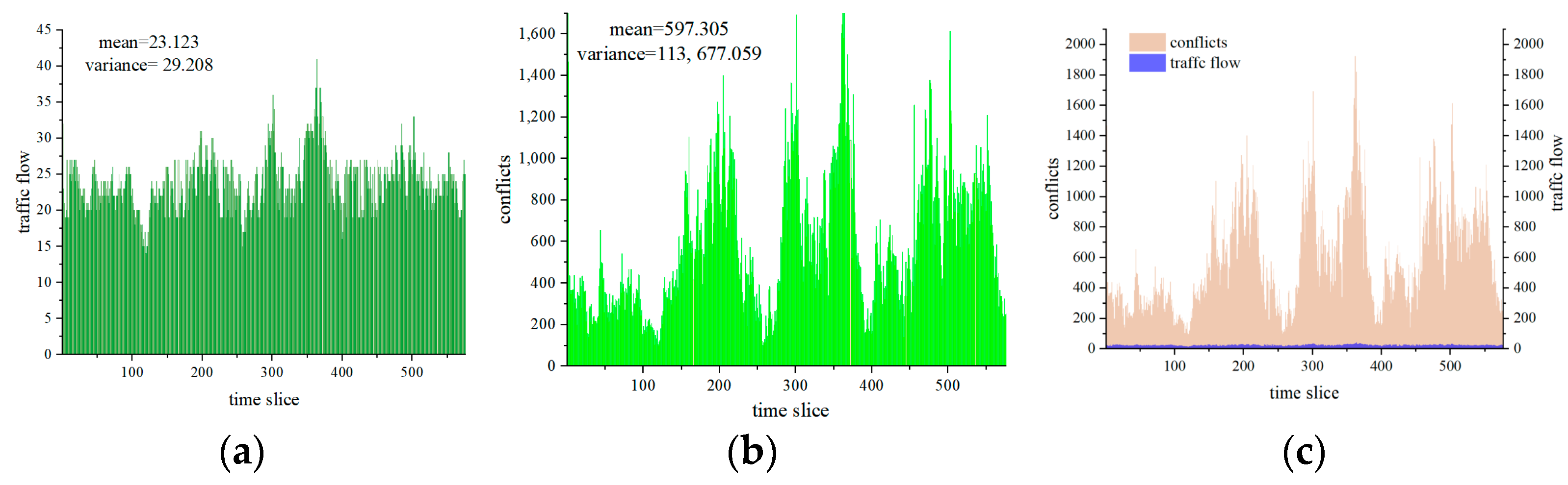
4.2. Analysis of Traffic Interactions Context

Taking Section a in Figure 10 as an example, we calculated the $conflicts$ for Section a every 5 min for a period of 2 days, where the $\lambda$ and $\delta$ parameters were set to 120 and 0.8, respectively, according to expert assessments. There are 576 time slices in this period. From Figure 12a, it can be observed that the traffic flow on the water’s surface exhibited time-varying characteristics. Compared with traditional traffic flow information, conflicts fluctuated more drastically, with a variance of 113,677.059 in Figure 12b, which is much higher than that in traffic flow. We used an unsupervised clustering method k-means algorithm to classify the surface state based on these two indicators. It can be found that the traffic flow can be divided into three states, and the conflicts more reasonably reflect the state of the water’s surface, which is divided into five categories, as shown in

Table 2. Congestion state based on traffic flow.

Congestion State	Smooth	Mild Congestion	Serious Congestion
Traffic flow	0–16	16–24	>24

and

Table 3. Congestion state based on conflicts.

Congestion State	Smooth	Basically Smooth	Mild Congestion	Moderate Congestion	Series Congestion
$conflicts$	0–183	183–438	438–811	811–1132	>1132

. It can be concluded that $conflicts$ can reveal hidden interactive information that traditional traffic flow does not capture.

We compared the two indicators in Figure 12c and found that $conflicts$ provide a more outstanding feature of surface situations over time. A high $conflicts$ value may demonstrate that vessels on the surface are relatively close even if there are few vessels. Incorporating more meaningful sources of information indicating the state of the water’s surface is essential to improving model performance and achieving better predictions of vessel travel time.

For a certain sub-trajectory, we incorporated four consecutive $conflicts$ values into our deep learning model, which represents the traffic interaction information of our prediction task, as clarified in Section 2.2.1. The traffic interaction information combines the latent feature information regarding sub-trajectories that has been extracted by the CNN. Then, LSTM is applied to learn the temporal relationships in a series of fused data in order to output the final travel time.

4.3. Travel Time Prediction Experiment

In this section, we present the training process and the results of the travel time prediction experiments conducted on the two test datasets. We introduce the evaluation metrics used in our model and compare the effectiveness of our model against classic travel time prediction models through comparison experiments. Furthermore, we report the results of an ablation experiment undertaken to demonstrate the superiority of our model.

4.3.1. Training of TTP-MTI

Training-related parameters’ settings: The number of epochs was set to 100, the learning Rate was set to 0.0001, and the batch size was preset to 32. The convolution kernel size was set to 3 × 3. MAE was used as the loss function for the Adam optimizer.

Running environment: The program was written in Python, and the model was built based on Keras and run on a GPU (Nvidia GeForce GTX 1060).

In order to train TTP-MTI, all of the trajectory pictures labeled in advance were divided into a training set (80%) and a test set (20%). To determine the best structure of the CNN, the performance of six different structural models with the same hyperparameters was compared based on the training set. The variables include the number of convolutional layers and the number of convolutional layer nodes, as shown in

Table 4. Comparison of different convolutional structures.

Structure	Number of Conv. Layers	Number of Nodes in Each Conv. Layer	Upstream MAE	Downstream MAE
A	2	32-32	0.351	0.342
B	2	32-64	0.336	0.295
C	3	32-32-64	0.231	0.228
D	3	32-64-64	0.254	0.247
E	4	32-32-32-64	0.289	0.263
F	4	32-32-64-64	0.272	0.266

.

As shown in Table 4, it is clear that the best structure is structure C, which presents the lowest MAE and consists of three convolution layers with a combination of nodes equal to 32-32-64. The training process is shown in Figure 13.

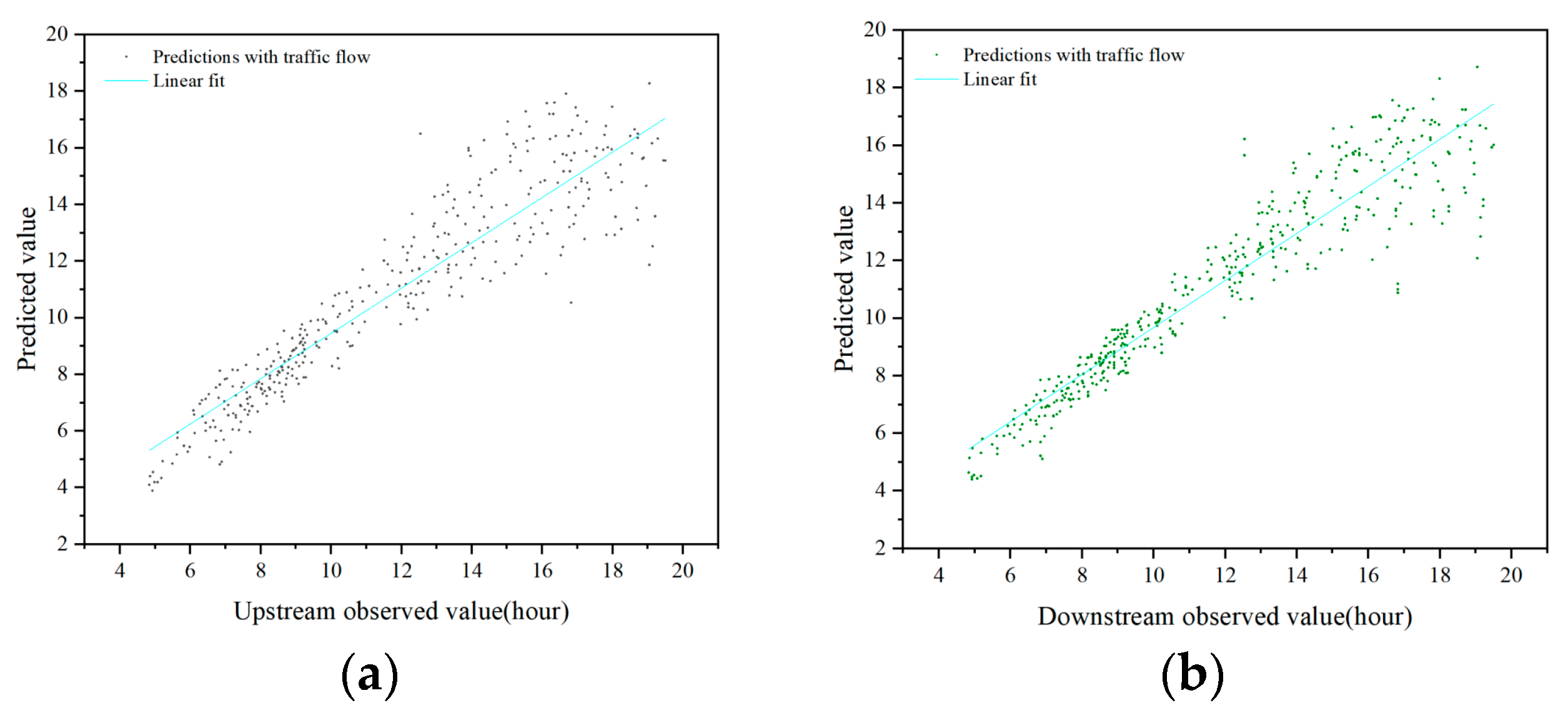
4.3.2. Travel Time Prediction Results

We evaluated the model’s prediction performance regarding inland vessel travel time when applied to the test set. To verify the effectiveness of the VCIN, we conducted a comparison experiment on two sets of traffic context information based on the optimal structure in Section 4.3.1: traditional traffic flow information and $conflicts$ as determined by the VCIN. The observations are shown in Figure 14; we analyzed the Upstream and Downstream separately to reveal the different prediction difficulties. The performance for the Downstream predictions was generally better than that for the Upstream predictions in all four scenarios. This is because upstream vessels flow against the current, making their speed more difficult to control, resulting in more random travel times. In contrast, downstream ships follow the current trend, enabling less resistance and faster speeds, leading to more stable and predictable travel times. Additionally, the prediction accuracy decreases as the prediction travel time increases. This can be explained by the fact that longer trajectories may entail more random turns or temporal stops, making travel time prediction more difficult.

Comparing Figure 14a,b with Figure 14c,d, it can be observed that our model leveraging the VCIN’s analysis significantly improves prediction performance in both upstream and downstream prediction tasks. While the traffic flow captures only static features and does not fully reflect the dynamic interactions of vessels impacting the vessel speed and travel time, the $conflicts$ metric successfully captures this detail and provides evolving information through its fluctuating value, leading to improved prediction accuracy. Specifically, a higher $conflicts$ value may indicate a longer travel time.

4.4. Comparison Experiment

In order to evaluate the effectiveness of our proposed model, we implemented it and compared it against four competing baselines described in the literature. The test set trajectories were chosen to demonstrate the capabilities of our model and baselines in various scenarios. The four models are explained below:

Speed/distance-based [3]: This model uses path-finding algorithms to predict the remaining route to a destination in order to estimate the remaining distance and then calculates the travel time by dividing the remaining distance by an estimated velocity. In our study, since the trajectories were provided in advance, we calculated the travel time by dividing the length of the trajectories by an estimated velocity.

SVR-based [6]: This model establishes a non-linear mapping relationship between the distance to the destination and the remaining travel time using the Support Vector Regression (SVR) model. This relationship does not consider intermediate speed and other processes and is an end-to-end model that includes six inputs of a vessel’s latitude, longitude, speed over ground, course over ground, navigation status, and remaining distance.

SPD-LSTM [19]: This model uses the traffic flow speed as context information and employs a section-based approach that utilizes Long Short-Term Memory (LSTM) for prediction, but it does not consider the traffic context information.

The results of the comparative experiment are presented in Figure 15. The Speed/Distance-based model showed poor performance across all metrics in both downstream and upstream prediction tasks. This simple method calculates the linear relationship between trajectory length and estimated speed, which proved inadequate due to fluctuations in speed in real-world scenarios. In contrast, the SVR-based model demonstrated improved prediction results by leveraging nonlinear regression techniques that model the relationship between travel time and distance. The SPD-LSTM model exhibited acceptable predictive ability across various metrics by learning dependencies from the input time-series information to make time-relative travel time predictions, but it did not consider the traffic context information. However, all these models were subject to insufficient contextual information, as travel time was affected by various factors such as the environment and vessel type. Our proposed model showed the best results in terms of three metrics compared to the baselines. The TTP-MTI model has been validated as a promising model for predicting inland vessel travel times since it considers the essential features of trajectory using CNN rather than just the length value, which indicates topographical structure information of an inland channel. Additionally, the fusion of traffic contexts also contributed to the final predictions. The predictability for upstream vessels is better than that for downstream vessels, and the analysis in Section 4.3.2 explains why: upstream vessels flow against the current and have a more random speed, while downstream vessels follow the current trend, leading to more stable and predictable travel times.

4.5. Ablation Experiment

To validate the effectiveness of the model architecture of the proposed deep learning model, we conducted an ablation experiment by comparing our model with variations for which one or more input modules are removed. We denoted the models as M1, M2, M3, and M, among which M is our complete model.

• M1 excludes vessel type, size, and power information, assuming all vessels are of the same type without incorporating additional distinguishing features;
• M2 excludes traffic interaction context information;
• M3 excludes date information in inputs;
• M4 only inputs the trajectory without the convolution process, leading to some redundant trajectory characteristics in the model.

The results of the ablation experiment are presented in

Table 5. Comparison of model performance.

Model	Upstream			Downstream
	MAE	RMSE	MAPE	MAE	RMSE	MAPE
M1	2.2567	2.9831	0.3223	2.0129	2.7294	0.3116
M2	2.1291	2.5784	0.2125	1.7861	2.5301	0.2084
M3	1.9122	2.2084	0.1971	1.3499	1.9836	0.1782
M4	1.9673	2.5562	0.2085	1.7221	2.5192	0.1943
M	0.4337	1.3095	0.1213	0.3894	1.2811	0.0937

.

It can be observed from the results of the ablation experiment that the prediction accuracy of M1 deteriorated sharply compared with our approach, which means that the vessel size and power information had the most significant impact on prediction performance. This is consistent with the common understanding that vessels have varying power capacities, which can greatly affect their average speed or travel time on a given route. M2 indicated that traffic interaction context information had an influence on travel time predictions. Date information (M3) did not have a significant impact on the prediction performance. Furthermore, the exclusion of the convolutional neural network (M4) decreased prediction accuracy, indicating that the convolutional neural network learned to extract useful trajectory features to support the prediction task. Overall, our proposed model exhibited the least prediction error compared to the ablation models, confirming the necessity and effectiveness of the designed deep learning prediction architecture.

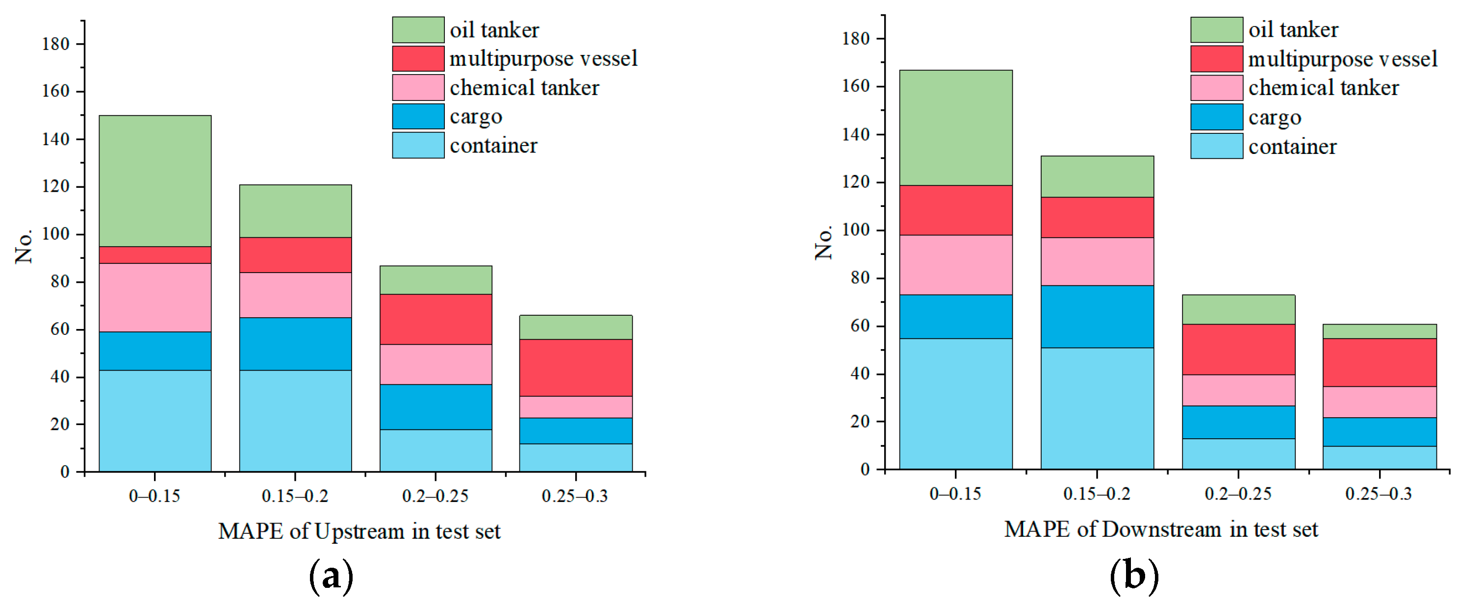
4.6. Error Distribution of Different Types of Vessels

As demonstrated in the ablation experiment above, the consideration of the vessels’ individual parameters, including type information, significantly improved the predictions. To further understand the predictability of different types of vessels, we computed the error distributions (MAPE) for different types of vessels in four intervals based on the test set, as shown in the statistical histogram in Figure 16. This analysis provides a deeper understanding of the model’s performance for various vessel types.

The five types of vessels analyzed—oil tankers, multipurpose vessels, chemical tankers, cargo ships, and container ships—were divided into four error intervals (0–0.15, 0.15–0.2, 0.2–0.25, and 0.25–0.3, respectively). As shown in Figure 16a, the proportion of oil tankers decreased with an increasing error, with 37% of vessels being oil tankers in the 0–0.15 interval. This indicates that the majority of oil tankers had good predictions and that their travel times were relatively easy to predict. In contrast, multipurpose vessels posed the greatest challenge, with their travel time proportion exhibiting an increasing trend. This may be because oil tankers often adopt fixed-point navigation for safety and economic reasons, thus other vessels will actively avoid approaching them, leading to a more stable movement process and easier time predictions. However, multipurpose vessels exhibit stronger mobility with greater uncertainty, making their prediction difficult. Similar trends can be found in Figure 16b. In conclusion, the predictions reveal that different vessel types have different levels of predictability performance.

5. Conclusions

This paper has addressed the issue of predicting travel times for inland vessels, which has been insufficiently studied in previous research due to a lack of traffic context information. We proposed a novel VCIN to capture the dynamic interactions between vessels, enabling the extraction of effective traffic interaction contexts. We also developed a deep learning prediction model that combines CNN and LSTM to determine the spatial features of trajectory and the dependency of section-based multiple fused data. Through a series of comparison experiments conducted on a real-world dataset from the Wuhan section of the Yangtze River, we have demonstrated the enhanced effectiveness of our proposed model compared to classic methods. Our ablation experiment further supports the superiority of our model’s design.

Future work could extend our model to solve the online travel time prediction problem through taking more uncertain factors into account, such as sudden accidents or collisions on the water. Moreover, collecting online crew manipulation actions and investigating their correlations with vessel travel time could also be a promising avenue of research.

References

1. Fancello, G.; Pani, C.; Pisano, M.; Serra, P.; Zuddas, P.; Fadda, P. Prediction of arrival times and human resources allocation for container terminal. Marit. Econ. Logist. 2011, 13, 142–173. [Google Scholar] [CrossRef]
2. Wu, X.; Roy, U.; Hamidi, M.; Brian, N. Estimate travel time of ships in narrow channel based on AIS data. Ocean Eng. 2020, 202, 106790. [Google Scholar] [CrossRef]
3. Alessandrini, A.; Mazzarella, F.; Vespe, M. Estimated Time of Arrival Using Historical Vessel Tracking Data. IEEE Trans. Intell. Transp. Syst. 2019, 20, 7–15. [Google Scholar] [CrossRef]
4. Park, K.; Sim, S.; Bae, H. Vessel estimated time of arrival prediction system based on a path-finding algorithm. Marit. Transp. Res. 2021, 2, 100012. [Google Scholar] [CrossRef]
5. Yu, J.J.; Tang, G.L.; Song, X.Q.; Yu, X.; Qi, Y.; Li, D.; Zhang, Y. Ship arrival prediction and its value on daily container terminal operation. Ocean Eng. 2018, 157, 73–86. [Google Scholar] [CrossRef]
6. Xu, X.; Liu, C.; Li, J.; Miao, Y. Trajectory clustering for SVR-based Time of Arrival estimation. Ocean Eng. 2022, 259, 111930. [Google Scholar] [CrossRef]
7. Sheng, Z.; Lv, Z.Q.; Li, J.B.; Xu, Z.H.; Sun, H.K.; Liu, X.; Ye, R.K. Taxi travel time prediction based on fusion of traffic condition features. Comput. Electr. Eng. 2023, 105, 108530. [Google Scholar] [CrossRef]
8. Peng, C.; Ding, C.; Lu, G.; Wang, Y. Short-Term Traffic States Forecasting Considering Spatial–Temporal Impact on an Urban Expressway. Transp. Res. Rec. J. Transp. Res. Board 2016, 2594, 61–72. [Google Scholar]
9. Fei, X.; Lu, C.C.; Liu, K. A bayesian dynamic linear model approach for real-time short-term freeway travel time prediction. Transp. Res. Part C-Emerg. Technol. 2011, 19, 1306–1318. [Google Scholar] [CrossRef]
10. Jiang, X.; Wen, X.; Wu, M.; Song, M.; Tu, C.L. A complex network analysis approach for identifying air traffic congestion based on independent component analysis. Phys. A Stat. Mech. Its Appl. 2019, 523, 364–381. [Google Scholar] [CrossRef]
11. Sui, Z.; Wen, Y.; Huang, Y.; Zhou, C.; Xiao, C.; Chen, H. Empirical analysis of complex network for marine traffic situation. Ocean Eng. 2020, 214, 107848. [Google Scholar] [CrossRef]
12. Houman, K.; Mobin, G.N.; Abbas, S.; Mohammad, K.; Mokhtar, M. Feature Selection and Training Multilayer Perceptron Neural Networks Using Grasshopper Optimization Algorithm for Design Optimal Classifier of Big Data Sonar. J. Sens. 2022, 2022, 9620555. [Google Scholar]
13. Sun, J.; Kim, J. Joint prediction of next location and travel time from urban vehicle trajectories using long short-term memory neural networks. Transp. Res. Part C. 2021, 128, 103114. [Google Scholar] [CrossRef]
14. Rong, H.; Teixeira, A.P.; Guedes, S.C. Data mining approach to shipping route characterization and anomaly detection based on AIS data. Ocean Eng. 2020, 198, 106936. [Google Scholar] [CrossRef]
15. Douglas, D.H. Algorithms for the reduction of the number of points required to represent a line or its caricature. Can. Cartogr. 1973, 10, 112–122. [Google Scholar] [CrossRef]
16. Wu, B.; Yip, T.L.; Yan, X.; Soare, C.G. Review of techniques and challenges of human and organizational factors analysis in maritime transportation. Reliab. Eng. Syst. Saf. 2022, 219, 108249. [Google Scholar] [CrossRef]
17. Duan, H.; Ma, F.; Miao, L.; Zhang, C. A semi-supervised deep learning approach for vessel trajectory classification based on AIS data. Ocean Coast Manag. 2022, 218, 106015. [Google Scholar] [CrossRef]
18. Xu, M.; Liu, H. A flexible deep learning-aware framework for travel time prediction considering traffic event. Eng. Appl. Artif. Intell. 2021, 106, 104491. [Google Scholar] [CrossRef]
19. Ma, X.; Tao, Z.; Wang, Y.; Yu, H.; Wang, Y. Long short-term memory neural network for traffic speed prediction using remote microwave sensor data. Transp. Res. Part C-Emerg. Technol. 2015, 54, 187–197. [Google Scholar] [CrossRef]
Figure 1. Workflow of our vessel travel time prediction via VCIN.
Jmse 11 01146 g001
Figure 2. Illustrations of channel centerline and DP algorithm on centerline.
Jmse 11 01146 g002
Figure 3. A VCIN explanation of a sub-trajectory. (a) Vessels without interactions (b) Two pairs of vessels have interacitons (c) Seven paris of vessels have interacitons (d) Weight calculation of each edge.
Jmse 11 01146 g003
Figure 4. Conflict extraction method for traffic interactions.
Jmse 11 01146 g004
Figure 5. One-hot encoding of categorical attributes.
Jmse 11 01146 g005
Figure 6. Framework for predicting travel time with multi-traffic information (TTP-MTI).
Jmse 11 01146 g006
Figure 7. Raw AIS data covering an area of 141 Km of Yangtze River.
Jmse 11 01146 g007
Figure 8. Speed distribution and AIS data after preprocessing.
Jmse 11 01146 g008
Figure 9. Vessel trajectory data based on AIS data.
Jmse 11 01146 g009
Figure 10. (a) Relationship between distance threshold of DP algorithm and number of retained key points in the channel’s centerline. (b) Visualization of key points.
Jmse 11 01146 g010
Figure 11. Sub-trajectories labeled with corresponding vessel types.
Jmse 11 01146 g011
Figure 12. Traffic context information of the Wuhan section from 9:00 on 11 December 2022 to 9:00 on 13 December 2022: (a) Traffic flow changes; (b) traffic interaction status changes represented by conflicts; (c) Comparison of the traffic flow and conflicts.
Jmse 11 01146 g012
Figure 13. The training process of TTP-MTI.
Jmse 11 01146 g013
Figure 14. Error comparison of different traffic contexts. The x-axis represents observed travel time, and the y-axis represents predicted value. (a) Comparison with traffic flow in Upstream set; (b) Comparison with traffic flow in Downstream set; (c) Comparison with VCIN in Upstream set; (d) Comparison with VCIN in Downstream set.
Jmse 11 01146 g014aJmse 11 01146 g014b
Figure 15. Comparison of MAE, MAPE, and RMSE. (a) MAE comparison; (b) MAPE comparison; (c) RMSE comparison.
Jmse 11 01146 g015
Figure 16. Error distribution of different types of vessels. (a) MAPE distribution in Upstream; (b) MAPE distribution in Downstream.
Jmse 11 01146 g016