1. Introduction
Unmanned surface vehicles (USVs) can be deployed in complex natural environments, replacing manned ships in numerous applications, such as rescue, disaster relief, and environmental monitoring [
1]. A closed-circuit television (CCTV)-system-based vision sensor is one of the conventional assemblies for USVs. Compared to laser rangefinder instruments, synthetic aperture radar vision sensors have extensive advantages, such as data richness, low cost, and good stability [
2,
3,
4]. A USV with autonomous navigation capabilities can ensure self-safe and efficient execution to complete specific tasks; in particular, the rapid development of visual navigation technology has laid an important foundation for autonomous navigation [
5,
6]. For long voyages, early determination of the sea level relies on visual navigation technology to help maintain USV balance and smooth navigation [
7,
8].
The horizon line detection operation is an essential foundation of visual navigation technology. In general, the area above the horizon line is represented as a contour dividing the background and the water, which encompasses the navigable area for the USV. Horizon line detection greatly affects the performance of subsequent steps, such as intelligent autonomous navigation, situational awareness, dynamic positioning, obstacle detection, and target tracking, and the entire navigation system plays an important role [
9]. Although many horizon line detection methods have been proposed for open-field environments, few methods are available for complex natural environments, such as harbours and inland rivers, and often the robustness and accuracy do not address the practical needs [
10]. How to extract the critical pixel points from the billions of raw pixels that make up a horizon line, whose accuracy and robustness in a natural navigation environment is unknown, still remains to be understood. For example, once there are reflections, obstacle occlusions, illumination changes, camera jitter, irregular waves, and other disturbances on the water surface, horizon line detection becomes quite a challenging problem [
11]. The horizon line is the boundary that distinguishes the background area from the navigable area. Accordingly, the navigable area determination problem can be equated to a horizon line detection operation, which is a hot research topic to improve the autonomy of USVs [
12]. Therefore, the problem of detecting horizon lines using intelligent CCTV systems for USVs is a topic of practical importance, which can help ships maintain balance, estimate their altitude, determine navigable areas, and identify obstacles to be avoided.
In the field of autonomous USV navigation, some typical approaches for horizon line detection have been successful in open waters [
13,
14]. However, real-time and accurate detection of the horizon line in complex environments also needs to address the following central issues: (1) There are challenges in distinguishing the sea and the sky with similar colours and low contrast, which is caused by the prevailing atmospheric and illumination conditions. (2) Horizon line detection methods are significantly different for single-frame images and dynamic videos. (3) A quick algorithm for horizon line detection needs to be explored for a moving USV in a cluttered environment. (4) Traditional horizon line detection approaches have poor generalization performances, and they often obtain unstable results. (5) When the horizon line is not completely straight or there are other straight lines that create interferences, low-resolution results may occur.
In this paper, we aim to address the above horizon line detection issues in a complex maritime scenario based on our previous work [
15,
16,
17]. For this, the criteria for defining a complex scenario need to be clearly defined as a first step, which will also document the various challenging scenarios. Second, a novel and efficient horizon line detection algorithm is developed based on minimal manual interactions. Finally, some experiments are designed to evaluate the performance with other state-of-the-art networks on the Singapore maritime dataset (SMD) [
18], maritime obstacle detection dataset (MODD) [
19], and our self-collected Yangtze River navigation scene dataset (YRNSD). In summary, the main contributions of this paper are as follows:
- (1)
We propose criteria for classifying a complex scenario using the grey level co-occurrence matrix (GLCM) to cover various challenging scenarios.
- (2)
We develop an efficient method based on a novel dynamic region of interest (ROI) approach to detect the horizon line in a challenging scenario for a moving USV.
- (3)
We show that it is possible to use weak manual interactions and autonomous feature extraction techniques to detect the horizon line for intelligent visual navigation.
The remainder of this paper is organized as follows. A review of the related literature for horizon line detection is presented in
Section 2.
Section 3 provides design considerations and preliminaries, including the criteria for complex maritime scenarios. The details of our proposed method are presented in
Section 4, which contains five steps, namely, classification of the scenario complexity, expanded ROI extraction, dynamic ROI matching, edge extraction based on Zernike moments and lower edge-point linear regression fitting. In
Section 5, the experimental results obtained with our proposed method are presented and compared with other relevant state-of-the-art approaches. The subsequent conclusions and future work prospects are given in
Section 6.
2. Related Work
Several approaches have been explored and reported for detecting horizon lines using onboard or onshore sensors. According to a review of the literature, the development of these approaches has progressed through three categories. The first category is the manual sifting of local features, which mainly uses colour, edge and texture information. For example, Ref. [
20] first converts an RGB image into a binarized image using an Otsu threshold segmentation algorithm, and then combines a Hough transform to find the longest line and treats it as the horizon line. Ref. [
21] extended Canny edge detection and a Hough transform to the field of horizon line detection. Similarly, Ref. [
2] obtained some candidate horizons based on a Canny edge detector a Hough transform and then used a voting method and picked the horizon with the most votes as the true horizon. The inherent drawback of such methods based on local features is their instability in complex maritime environments, because the parameter selection relies on artificial empirical prior knowledge or underlying assumptions ([
22,
23]). For example, edge information easily suffers more in the presence of edge gaps, and texture information is easily blocked by local shadows and obstructions. Although edge gap filling processes have been proposed, it is also easy to get into trouble when the edge gap is larger than the search window.
The second category is adaptive global features. Most of the methods in this class are based on the overall features of an image and do not rely on prior knowledge, and these methods outperform the local feature methods ([
24,
25]). The extreme values of the gradient change are first sampled for each vertical column in the gradient image, and then the random sample consensus (RANSAC) method is used to fit the horizon line. Ref. [
26] proposed a hierarchical horizon detection algorithm that combines a Canny edge detector with a Hough transform to adaptively find the longest line and then fine-tunes it to obtain the horizon line information. Ref. [
27] extracted a rectangular region above a virtual horizon as a region-growing seed, and the region-growing algorithm helped obtain the final horizon. The overall features include colour distribution, texture information, and spatial context, and they can only be used as a basis for rough-level segmentation, as these features and principles may not be suitable for complex marine environments. Meanwhile, these methods still suffer from a homogeneous distribution problem in the water surface case, and there are local regions with abnormal changes in grey values that can reduce the accuracy, such as water surface shadows and obstacle occlusions.
The third category is intelligent detection methods, also called regression-based approaches. This class of approaches tends to use a coarse-to-fine strategy, i.e., initially focusing on the overall structural information and subsequently updating features using the finer details to provide more accurate predictions. Horizon line predictions use semantic segmentation based on deep learning ([
28,
29,
30]). The key is transforming horizon line detection into clustering and classification. At the same time, logistic regression and polynomial spline modelling are less effective in treating the probability distribution and physical characteristics of a detected horizon line. Depending on the degree of manual labelling for the training data, these approaches can be subdivided into semisupervised and supervised learning ([
31]). For example, Ref. [
32] designed a semisupervised water region segmentation learning method for USVs in a changing unknown environment by using automatically labelled training data with the aid of LiDAR. Ref. [
11] combined a multiscale approach and a convolutional neural network (CNN) to detect the horizon in maritime scenarios. In general, a horizon line extraction has two parts, a region of interest (ROI) extraction and horizon line estimation, where the important features are extracted first and then trained with intelligent detection methods. The vast majority of the above methods have been proven to be robust and accurate in general environments but have poor generalization performances for complex visual navigation environments, such as when mirror reflections exist on the water surface, or during water fogging or obstacle interference.
3. Design Considerations and Preliminaries
Before performing an accurate horizon line detection, we must differentiate the actual navigational environment captured using a CCTV system to determine whether the USV’s navigational scenario is in open water or complex water. Open-water scenarios are usually defined as outer waters with a wide field of view, making the horizon line detection relatively simple. However, complex water scenarios are usually inland rivers and harbours with heavy traffic, where the detection of horizon lines for complex scenarios is susceptible to numbers factors.
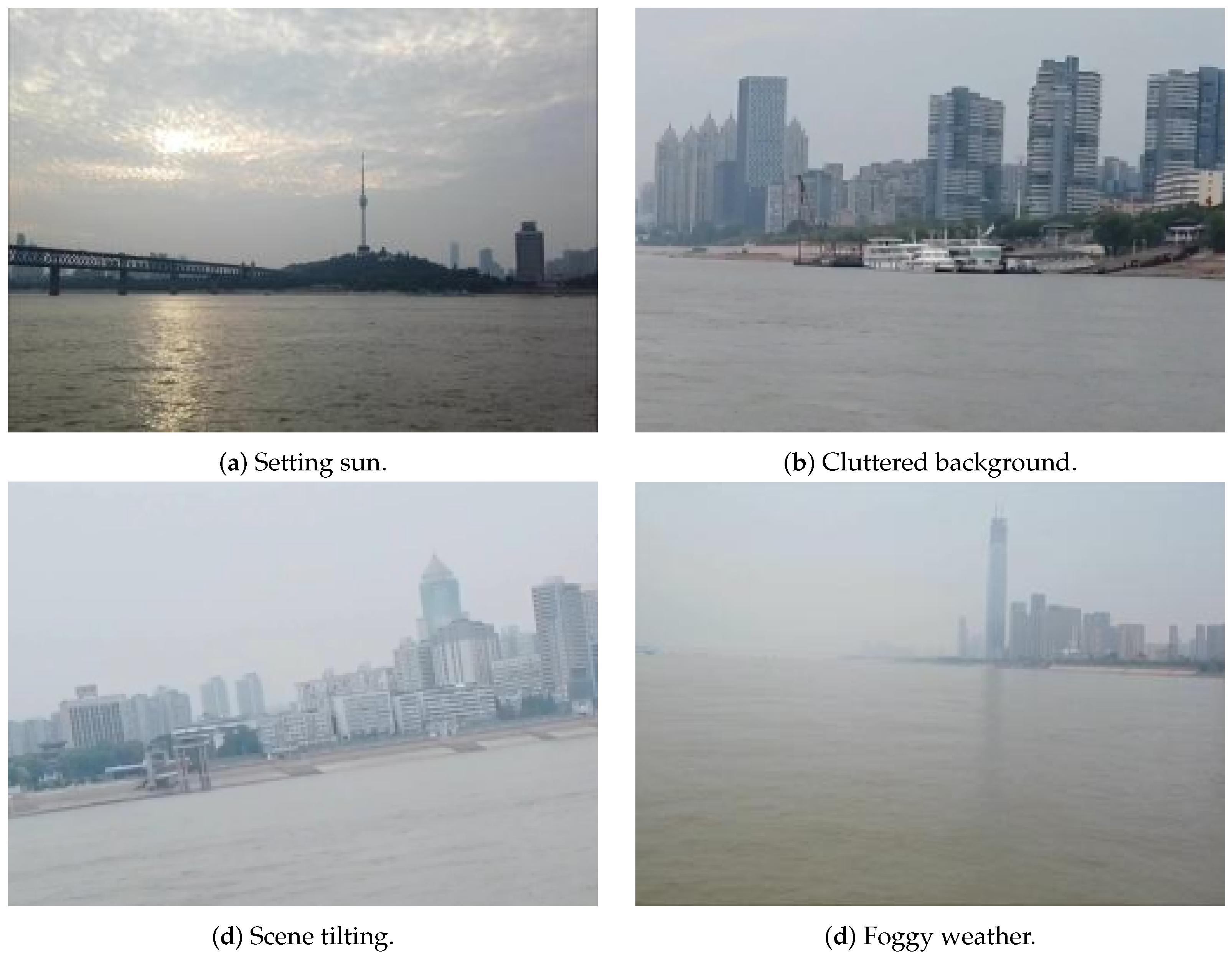
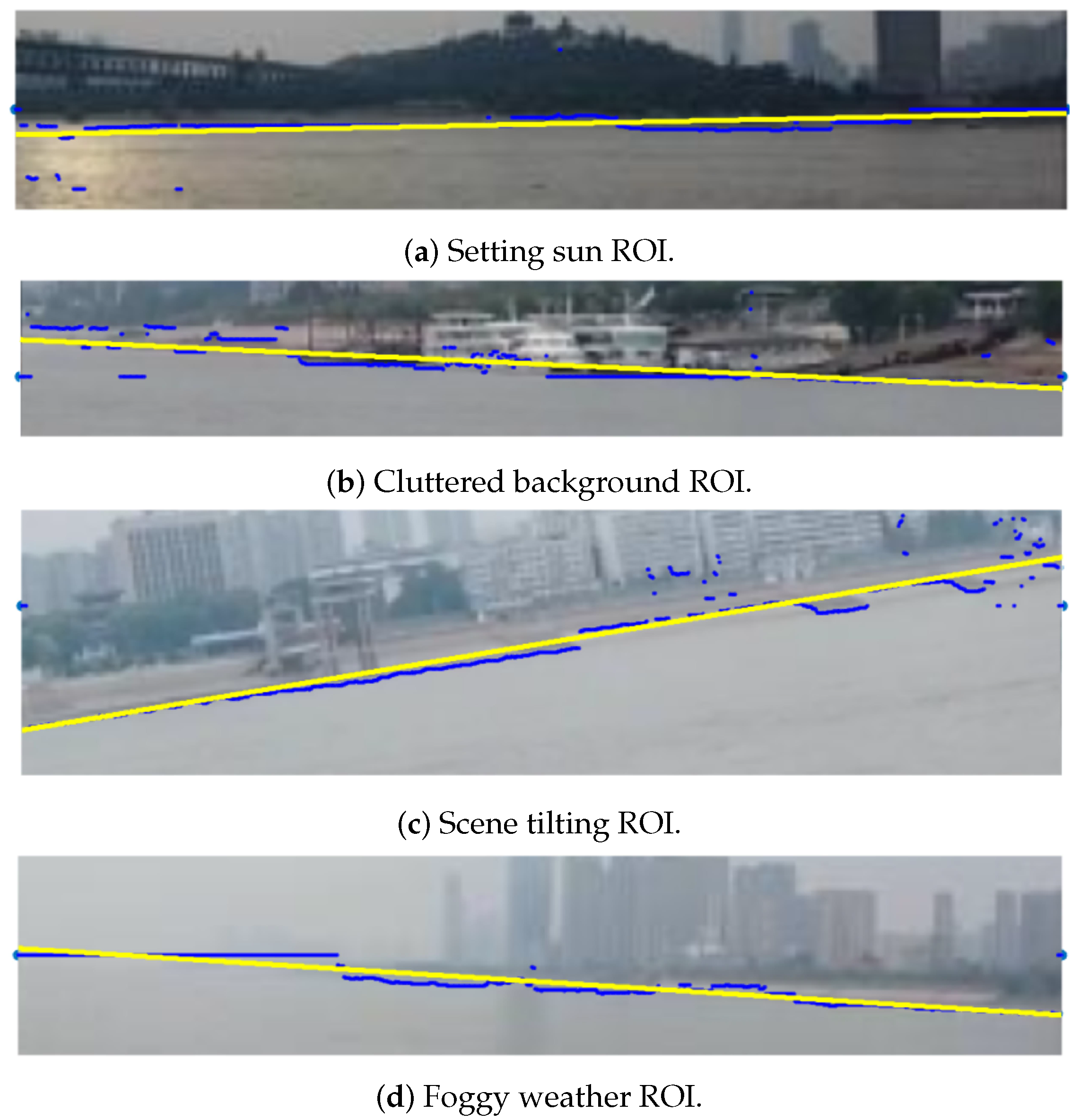
First, the water surface is susceptible to extremely dark or bright areas due to direct sunlight or reflections. For example, object shadows are formed when the light shining on the surface of an object is partially or completely blocked ([
33]). In addition to the effect of light projection, the reflection of the sun on the water surface can create large patches of extremely bright light that considerably block the continuity of the horizon line, as shown in
Figure 1a. Second, complex scenarios are bound to have other ships, floating objects, navigation aids, and other types of cluttered background, as shown in
Figure 1b, which disrupt the continuity of the horizon line features. When there are multiple obstacles blocking each other, horizon line detection will be even more challenging. Third, USVs are usually lightweight vessels, and when they are moving quickly, it is difficult to maintain the balance of the hull in a sustainable manner, resulting in a certain angle of tilt of the horizon line (as shown in
Figure 1c), which may be random and unpredictable. In addition, special weather conditions, such as night, rain, snow, and fog, can also affect the accurate extraction of the horizon line. As shown in
Figure 1d, foggy weather can cause the distinction between the water area and the background area to be blurred. As a result, the image information captured in complex scenarios is more complex and does not have a clear distinction between the water area and the background area compared to open water. Therefore, complex scenarios and their determination criteria are defined before conducting a horizon line detection to facilitate the coverage of a variety of challenging scenarios.
4. Proposed Approach
4.1. Classification of the Scenario Complexity
A spatial relationship is considered to be a function of the distance between two pixels, and the texture features extracted from a camera image using a grey level co-ocurrence matrix (GLCM) [
34] can be used to differentiate between navigation scenario complexities. Before the construction of the GLCM, we need to transform the original navigation scenarios into grey-level images. Assume an
navigation scene
I is transformed into a grey image
, which is described as:
is an image with
grey grades, and
and
are two pixel points in scene
with distance
d in the direction of
. Then, the GLCM of this navigation scene is calculated as follows:
where # denotes the number of elements in the set.
represents the grey levels of two pixels. The angular second moment (ASM) is one GLCM feature, which is often used to describe the uniformity of the greyscale distribution in images. The ASM is calculated as follows:
When the distribution of elements in the GLCM is more concentrated around the main diagonal, a smaller ASM indicates a more uniform distribution of pixel greyscales and finer textures; conversely, it indicates an uneven distribution of pixel greyscales and coarser textures. Hence, we use the ASM value as a criterion to determine the complexity of the scenario in this paper.
4.2. Expanded Region-of-Interest (ROI) Extraction
As the valuable information containing the horizon line feature points is usually concentrated in the central region of the whole image, if all the pixels of the whole image are traversed for the search calculation, it is not only computationally time-consuming but also difficult to meet the real-time requirements, and it introduces a large amount of unnecessary noise interference, which increases the image processing difficulty. Therefore, region-of-interest (ROI) extraction is a necessary operation for image processing.
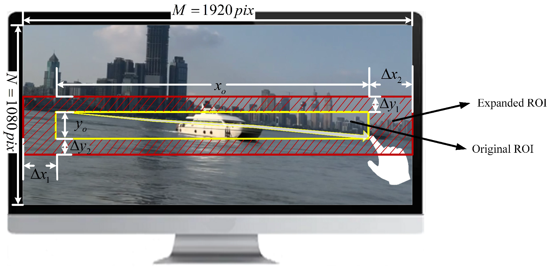
As shown in
Figure 2, to simplify horizon line detection, an original ROI defining a bounding box (yellow) around the touched line must be drawn by the user. Due to the small size of the display and the jittering hands of the user, the ROI is properly expanded as the the red bounding box. The following relationship exists between the expanded and original ROI:
where
and
denote the width and height of the expanded ROI, and
and
denote the width and height of the original ROI, respectively.
and
represent the expansion of the ROI compared to the original ROI in the horizontal and vertical directions, respectively. The image captured by the vision camera is of a
resolution, with three-channel RGB. In the actual processing, the width of the expanded ROI
is
M, which is the width of the captured image. Usually, the values of
and
can be unequal, i.e., the user is not required to manually draw the original ROI as horizontally centred. However,
and
are generally equal and take values of 20 pixels unless the size of the expanded ROI exceeds the boundary of the captured image, in which case the upper/lower boundary of the expanded ROI is taken directly from the upper/lower boundary of the captured image. The value of
is approximately equal to one-fifth of
N.
4.3. Dynamic ROI Matching
Using an interactive-based expanded ROI extraction strategy, the expanded ROI to be selected for a horizon line detection can be reduced. Unfortunately, it is also impractical to perform interactive ROI extraction for every frame because the workload is undoubtedly huge for video images of at least 25 frames per second (FPS). Considering that video images captured by the shipboard camera are continuous sequences containing time-stamped information, there is strong spatial continuity between the sequence images over a short time interval. Therefore, we only select the first image frame for interactive ROI extraction in the initialization phase of the algorithm, which is a minimal interaction that is usually acceptable in a crowdsourcing approach. The specific process of dynamic ROI matching is as follows:
Step 1: Initialization of the master areas. The expanded ROI
in the first video frame of the shipboard camera acts as the master areas.
is coregistered until all the video images are registered.
Step 2: Coarse extraction of the keypoints. The keypoints
of the master areas
and
are initially extracted using the oriented features from a accelerated segment test (oFAST), which introduces the concept of feature orientation to achieve the feature point rotation invariance.
Step 3: Fine extraction of the keypoints. Construct the Hessian matrix for the keypoints and finely extract
again to select the keypoint with better traceability. For the keypoints
, the following two conditions need to be met simultaneously:
where
and
both represent the Hessian matrix discriminant.
indicates the set threshold value. Equation (
7) implies that while the Hessian matrix discriminant of
is a local maximum, the sum of their differences needs to be greater than
.
Step 4: The keypoint descriptor. After a fine extraction of the keypoints, we use the rotated binary robust independent elementary features (RBRIEF) operator to compute the feature descriptors. The RBRIEF descriptor is constructed from a set of binary intensity tests.
Step 5: ROI matching. Brute force (BF) descriptor matching assigns the closest descriptor of the slave areas to the master areas. The power of BF matching lies in its ability to retrieve the nearest neighbours with a high probability given enough hash tables.
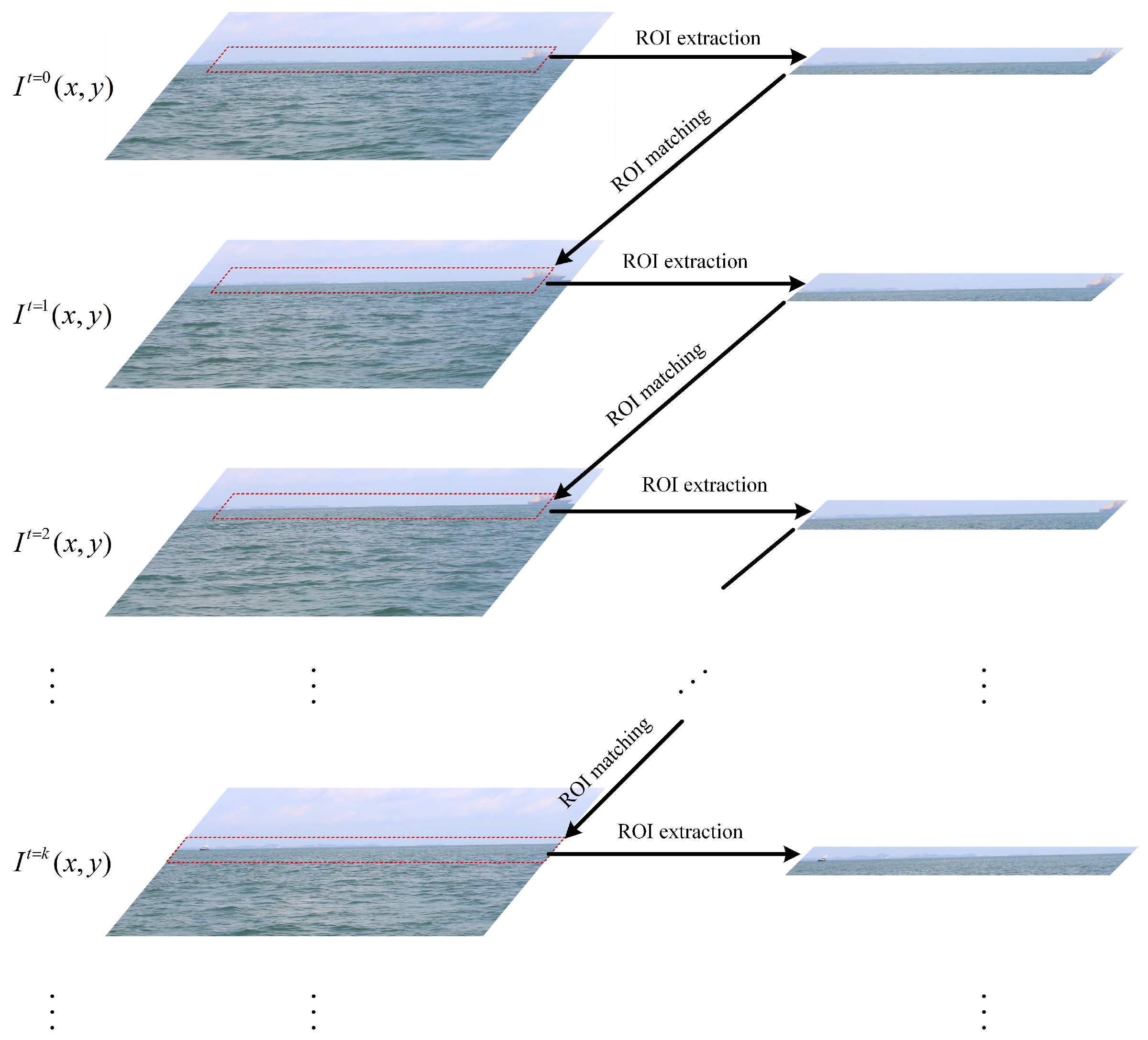
The horizon line candidate regions can be obtained continuously after the above five processing steps. As shown in
Figure 3, the spatiotemporal similarity between the upper and lower frames is used to dynamically locate the ROI.
4.4. Edge Extraction Based on Zernike Moments
After the dynamic ROI area has been extracted, the navigational scene needs to be further processed to obtain the horizon line information. Considering the poor robustness of the traditional Sobel and Canny operator edge detection algorithms against noise and image rotation, this study uses Zernike moments to extract the image contour edge. Zernike moments are a type of convolutional integration method that is highly resistant to noise interference and is rotationally invariant.
First, the two-dimensional Zernike moments of the ROI region can be defined as:
where
m and
n are two integers,
, and the value of
is an even number.
is the position of the edge of the image, while
.
is the angle between the X-axis and
.
means the ROI region.
is a Zernike polynomial of order
n, defined as a function of
and
in the polar coordinate system.
is the conjugate complex number of
.
Second, the paper directly refers to the classical
template factor calculated in [
35]
. Let the ROI region
, and note that the template of
is
; then, we have:
Then, Equation (
9) is utilized to calculate the templates and each pixel point of the ROI region image for the convolution operation to obtain
Zernike moments:
.
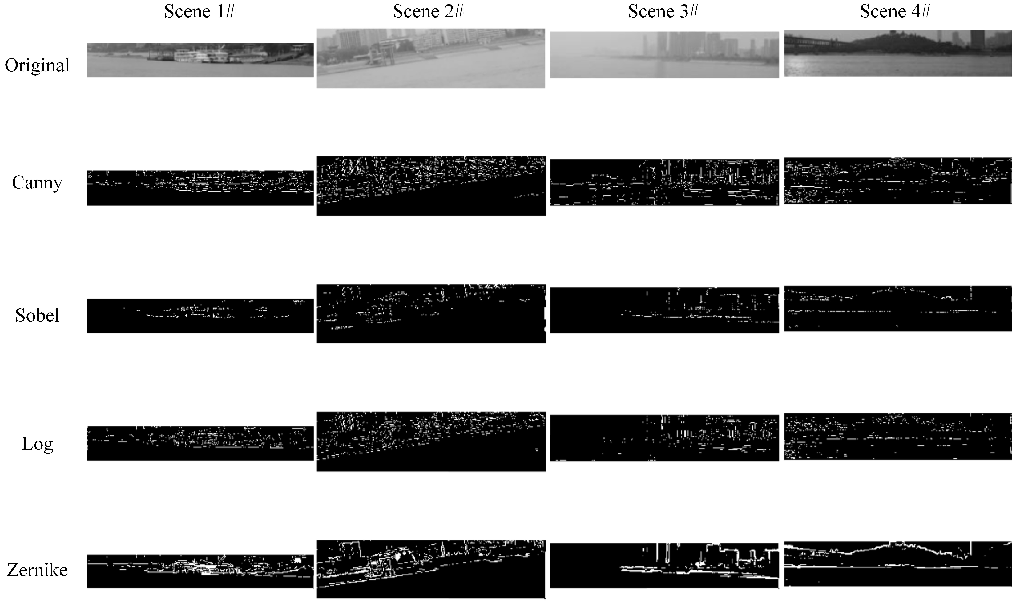
Finally, using the rotational invariance principle of the Zernike moments and edge points, the spatial greyscale model of edge points can be solved to find the pixel positions of the edge points in the ROI region.
Figure 4 shows the results of different edge extraction algorithms, where the ROI regions (Scene 1#, Scene 2#, Scene 3#, Scene 4#) come from
Figure 1.
4.5. Lower Edge-Point Linear Regression Fitting
The ROI region can be roughly located using edge detection based on the Zernike moments; however, further linear fitting is required to obtain a more accurate horizon line. Due to the influence of water spots, obstacles, complex backgrounds, and foggy weather, edge areas are often uneven and haphazard, which poses a great challenge for fitting the horizon line directly. To this end, the analysis of many edge images shows that there is usually a clear differentiation between the background area and the navigable water surface area, i.e., edge noise is usually distributed in the background area, while there are no edge points in the navigable area. Therefore, in this paper, by performing lower edge-point tracking on the edge points in the background region and putting the tracked points into the set
, we obtain the specific tracking process in Algorithm 1.
| Algorithm 1 Lower edge-point tracking algorithm |
| Require: The binarized image after Zernike moments edge extraction |
| Require: The number of rows of the ROI region M |
| Require: The column number of the ROI region N |
| Ensure: The set of |
| 1: while do i denotes the number of columns currently searched |
| 2: while do j denotes the number of rows currently searched |
| 3: if then |
| 4: Put the point into the set |
| 5: Break |
| 6: end if |
| 7: |
| 8: end while |
| 9: if then denotes that no edge points exist in this column |
| 10: Put the point into the set |
| 11: end if |
| 12: |
| 13: end while |
| 14: Return |
The linear regression method is used to fit the traced lower edge points
. A fitted linear equation
is first constructed, and the fitted linear function
is found so that the sum of squares of the errors with the actual value is minimized, and the objective function is:
where
is the weight of the lower edge point, and the initial weight of each edge point is 1 in Equation (
11).
Next, the weights of the edge points are updated according to the weight function, and the residual value
of the fitted line is calculated by fitting the equation of the line and the distance from the edge point to the fitted line. The weights of the lower edge points that deviate from the line should decrease as the residual
increases, and at the same time, the amount of weight function design computation is reduced, as follows:
where the reciprocal of the residual value is used as the weighted value of the lower edge points when the residual value is not zero.
Finally, the updated weight values are substituted into Equation (
10) using the least squares method to solve for the estimated horizon line information, and the specific effect is shown in
Figure 5. The ROIs in
Figure 5 are derived from
Figure 1, where the blue points are the traced lower edge points and the yellow lines are the horizon lines.
5. Experiment and Results
5.1. Datasets and Evaluation Metric
To verify the effectiveness of the proposed method, experiments were conducted on the SMD [
18], MODD [
19], and YRNSD datasets [
6], of which the first two are classical datasets and the third is a self-collected dataset. The SMD dataset was collected in Singapore waters from July 2015 to May 2016 under various environmental conditions, such as before sunrise (40 min before sunrise), sunrise, midday, afternoon, evening, haze and rainfall, and after sunset (2 h after sunset). The MODD dataset was collected in Koper Bay, Slovenia, using a camera fixed to an unmanned boat over a period of approximately 15 months, with the camera capturing video at a given resolution at 10 frames per second. The self-collected YRNSD dataset in this paper was captured in the Wuhan section of the Yangtze River basin and consists of 64 videos, which cover a wide range of types of obstacles and meteorological conditions. The experimental environment in this paper is an Intel Core i7-8700K CPU 3.70 GHz*12, NVIDIA GeForce GTX 1080Ti GPU, 32 GB RAM.
To quantitatively compare the performance of the methods, the
was employed to evaluate the complexity of the scene. In general, we consider that a larger
value represents a more complex navigational scene image and a greater difficulty in performing horizon line detection. The calculation of the
value can be used as a basis for choosing to use this method or a conventional edge detection before performing a specific horizon line detection.
Table 1 shows the distribution of
values corresponding to the three datasets.
As seen from
Table 1, the ASM value variation range for the same video scenes is small, as reflected by the small maximum ASM value variation ranges and their small standard deviation, indicating that the ASM values are relatively stable.
5.2. Impact of Different Complexity Levels
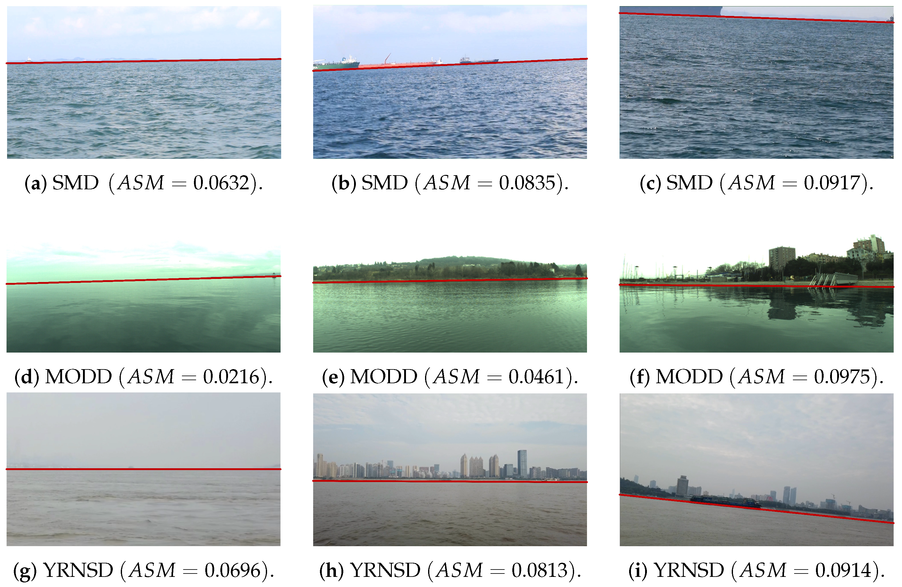
The complexity of the textures contained within each dataset also varies, so all the scene images are classified into low, medium, and high complexities, and specified as less than 25% (lower quartile), the 25% to 75% interval, and the greater than 75% (upper quartile) respectively.
Figure 6 shows 9 images derived from the 3 datasets.
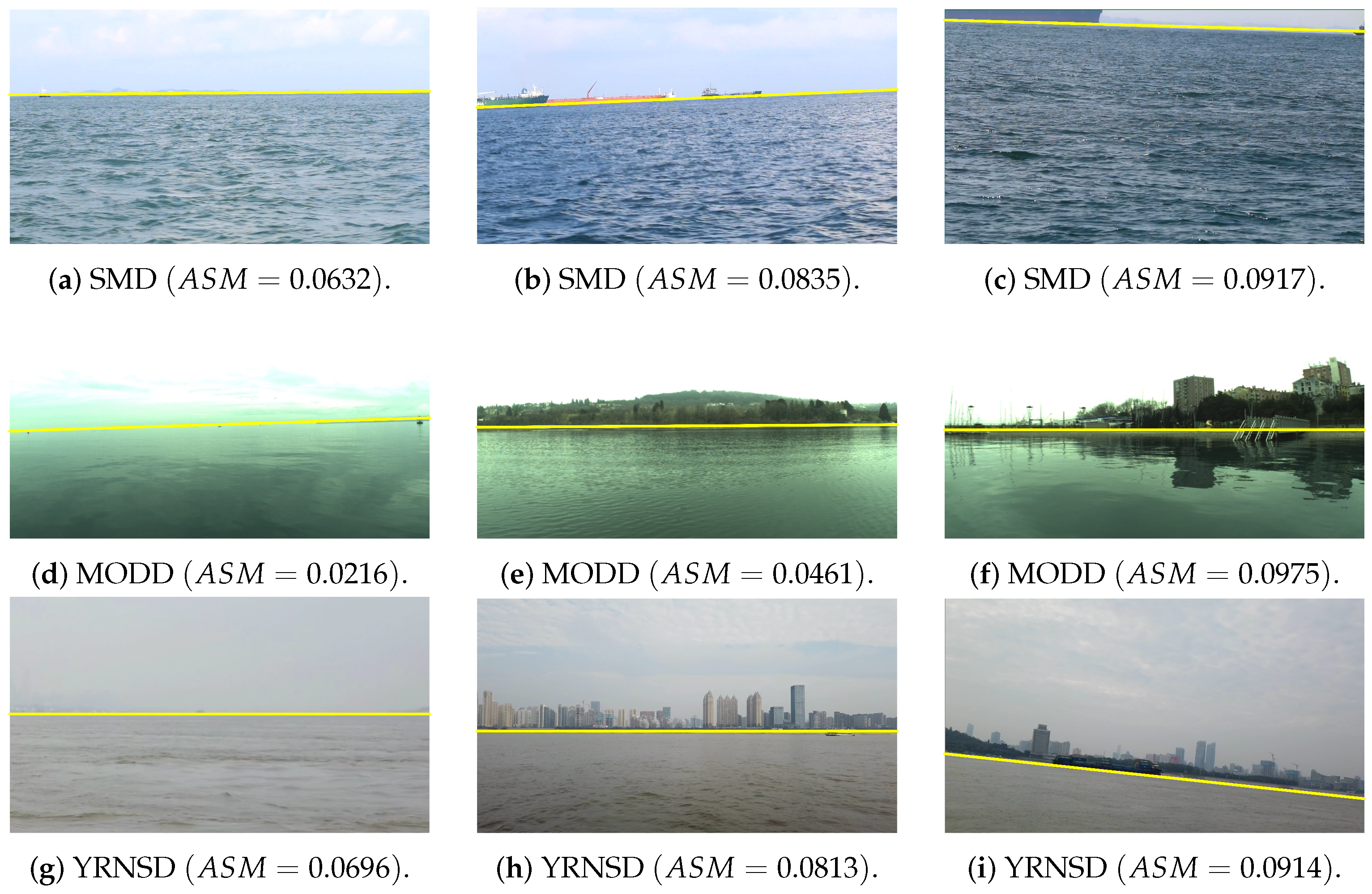
To quantitatively verify the accuracy of the proposed method, we extracted the horizon lines, point by point, for each of the 9 images in
Figure 6 by using manual annotations and used them as the real horizon line, and the extraction results are shown as the red straight lines in
Figure 6. Meanwhile, the horizon line information is obtained using the method in this paper, and the effect is shown as a yellow straight line in
Figure 7. Then, the average error
e between the detection result and the real result is calculated as Equation (
12), and the results are shown in
Table 2.
where
denotes the longitudinal coordinate of the
horizon line points detected by the proposed algorithm.
denotes the real longitudinal coordinate of the
horizon line points.
n denotes the number of horizon line points.
As seen from the results in
Table 2, the average algorithm error for scenes of different complexity from the three different datasets is within 2 pixels, indicating that the horizon line detection results of our method are very close to the real results, and the impact of different complexity scenes on this method is small. This is because we detect the region of interest in advance, and the complex background interference is already removed. Moreover, except for the initial region, which needs to be calibrated the first time it is used, all subsequent detection operations can be carried out automatically.
5.3. Comparative Analysis of Different Methods
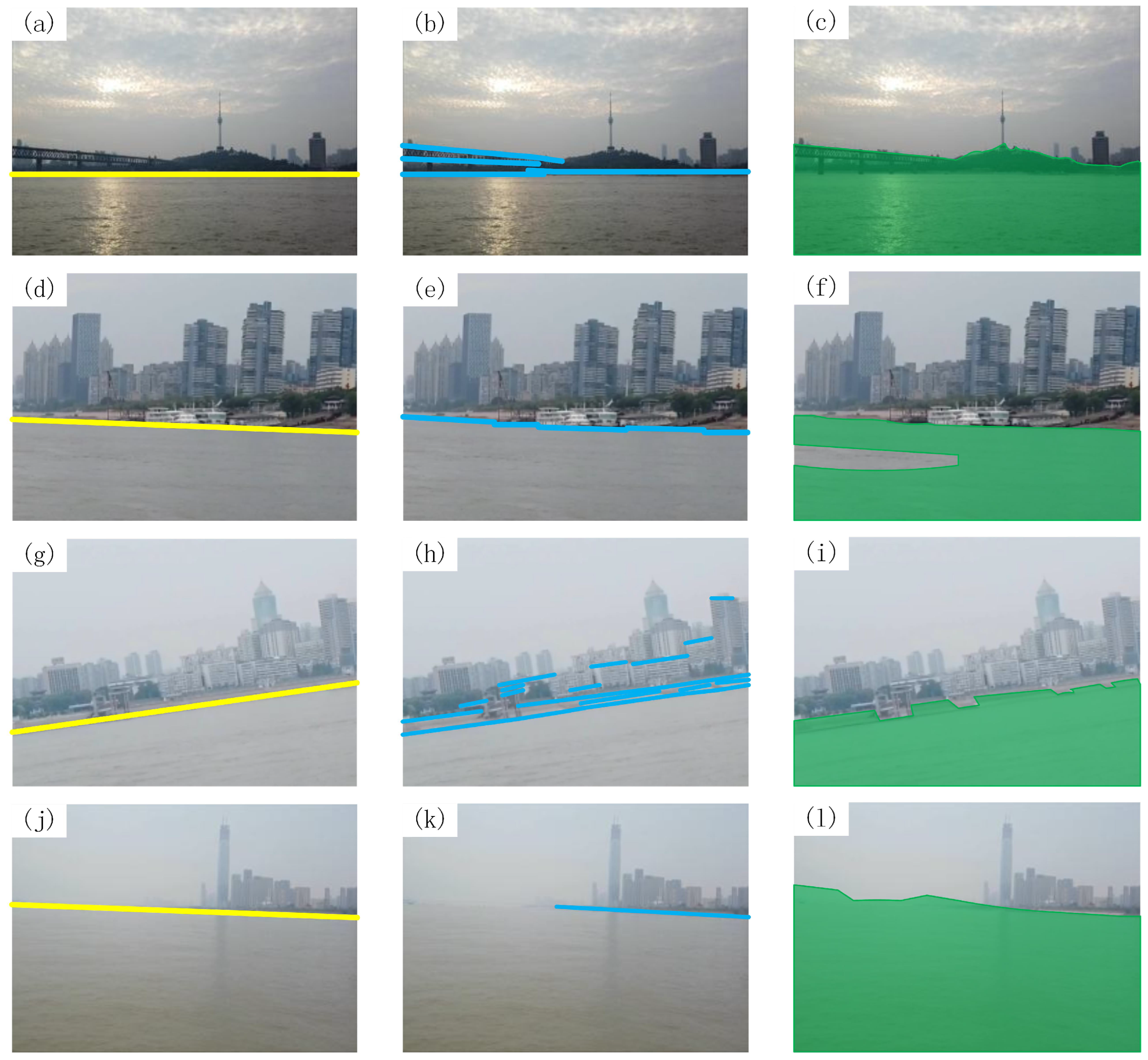
To further verify the methods performance, we compared the same images using the proposed method, the conventional edge detection and threshold segmentation methods (EDTSM), and the semantic segmentation methods (SSM), and the results are shown in
Figure 8.
Figure 8a,d,g,j show the horizon line detection results obtained using the proposed method;
Figure 8b,e,h,k show the horizon line detection results obtained using the conventional EDTSM; and
Figure 8c,f,i,l show the horizon line detection obtained using the SSM.
From the above experimental results, it can be concluded that the proposed algorithm is able to detect the horizon line relatively accurately, even under scenarios such as a setting sun, cluttered background, scene tilting and foggy weather images. The horizon line detected by traditional EDTSM-like methods often consists of multiple discontinuous line segments, and horizon line detection will fail in scenarios with high background complexities, cluttered edge information, and bad weather (e.g., foggy days). Although the recent trend of semantic segmentation for extracting horizon lines is effective and has a certain ability to improve the anti-interference capability compared to the EDTSM-like methods, most of these methods need a large amount of manually labelled data, and it takes a long time from training and testing to application deployment.
We employed our method on the R2018b Matlab platform to process a 2 min video sequence (obtained from the YRNSD dataset). The horizon line detection time took approximately 40 s, which also included the selection of initial frames of ROI that took about 10 s. Excluding the manual interaction period, the average detection time per frame was roughly 0.213 s. On the other hand, EDTSM-like methods under similar conditions took about 15 s and an average processing time of 0.12 s per frame while providing subpar accuracy in complex environments. The SSM-based method may be applied directly to process the same video sequence without requiring prior training, which takes approximately 38 s of processing time. This translates to 0.317 s per frame image. However, similar to edge-based methods, the horizon information extracted via SSM may not be precise enough in complex scenes.
In a comprehensive comparison, the proposed method is a coastline extraction algorithm based on minimal manual interaction, which definitely used less computational resources than the method based on SSM. Our method first performs an upfront calculation of the complexity of the scene, in addition to extracting the initial ROI using manual annotation and subsequent matching. These three steps are time-consuming but greatly reduce the region to be searched in the specific edge extraction phase, which can save some time. Moreover, for conventional EDTSM-like-method algorithms, which take the least amount of time, our method is able to obtain more accurate edge information, which is of the utmost importance. Therefore, for a USV with a long navigation time, the method in this paper can help obtain relatively accurate information about the horizon line in real time.
6. Conclusions
We proposed a horizon line detection method based on minimal manual interaction, which specifically includes evaluating the complexity of the navigation scene using the ASM parameters of GLCM. For highly complex scenes, we use manual interactions to dynamically extract the ROI in the initialization phase of the method, and then use key feature points to match the ROI in the next image frame as a way to continuously exclude the interference of the complex background environment. We then use Zernike moments to extract the edge features of the current ROI, and finally use the method of least squares to linearly fit all the lower edge feature points to the horizon line. To evaluate the effectiveness of our method, comparative experiments were designed for navigation scenarios of different complexities, also quantitative comparisons were conducted between this paper and the conventional EDTSMs and SSMs. Our experiments show that this method has the potential to be applied to the autonomous navigation and control of USVs.
Our method partially solves the problem of horizon extraction in complex environments but has some shortcomings. At present, the anti-interference and stability of our approach are poor in some extreme or unexpected situations. For example, during the long-term navigation of a USV, the front camera is frequently disturbed by water splashes, resulting in unclear images and failure of the dynamic region-matching algorithm to converge, leading to the failure of the horizon line extraction. In addition, as the endurance mileage of USV becomes longer, errors in the horizon line extracted by the linear fitting algorithm at the early stage may accumulate, requiring manual correction during the journey. The above two aspects are the main shortcomings of our method. In the future, we will focus on improving the anti-interference and stability of our approach. Specifically, we will concentrate on improving the hardware part of the image acquisition device to address the problem of susceptibility to water splash disturbance, and explore new discrete point-fitting methods to improve the long-term stability of the algorithm.


