
Vibration Suppression Trajectory Planning of Underwater Flexible Manipulators Based on Incremental Kriging-Assisted Optimization Algorithm

Abstract
:1. Introduction
2. Materials and Methods
3. Vibration Suppression Trajectory Planning
3.1. Cubic Polynomial Trajectory Planning
3.2. Constraint Condition
3.3. Objective Function
4. Optimization Algorithm
4.1. PSO Algorithm
4.2. Sparrow Search Algorithm (SSA)
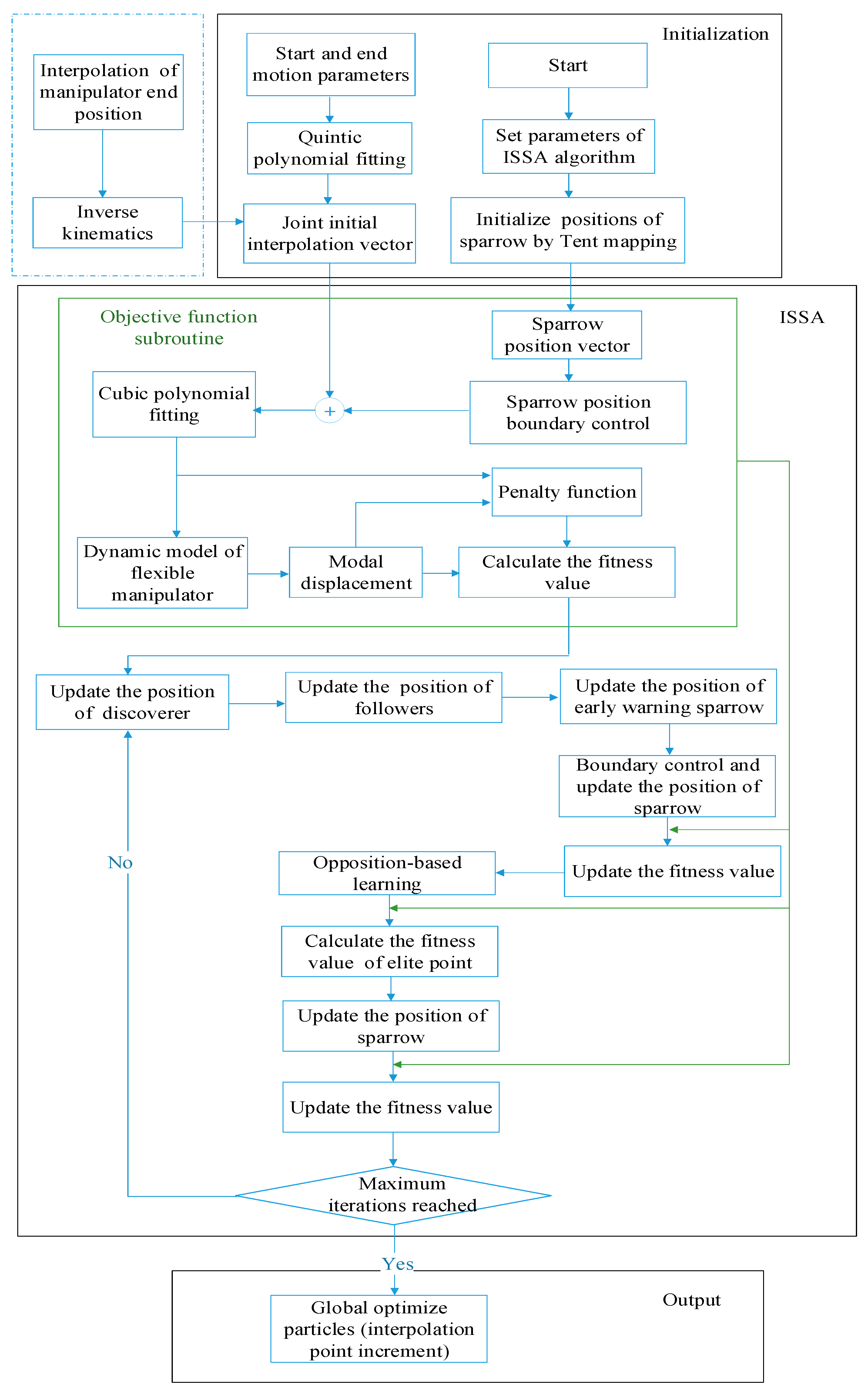
4.3. Improved Sparrow Search Algorithm (ISSA)
4.4. Simulation
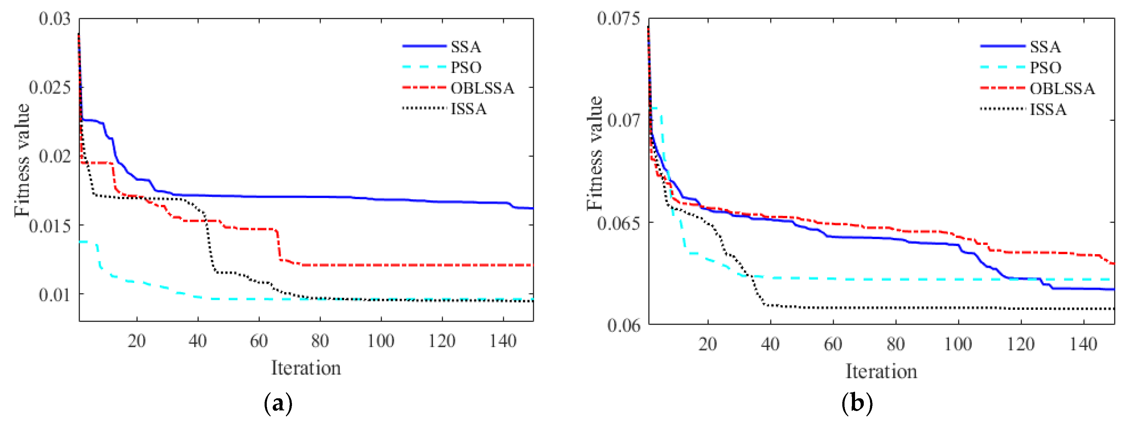
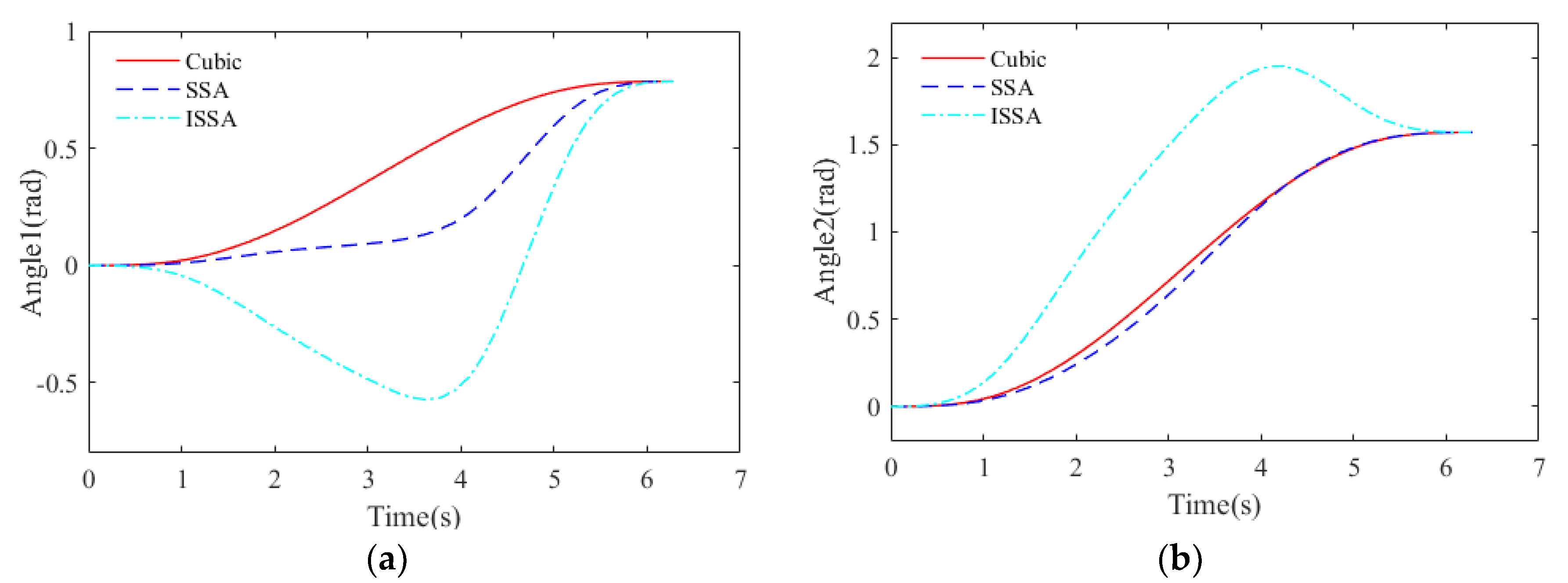
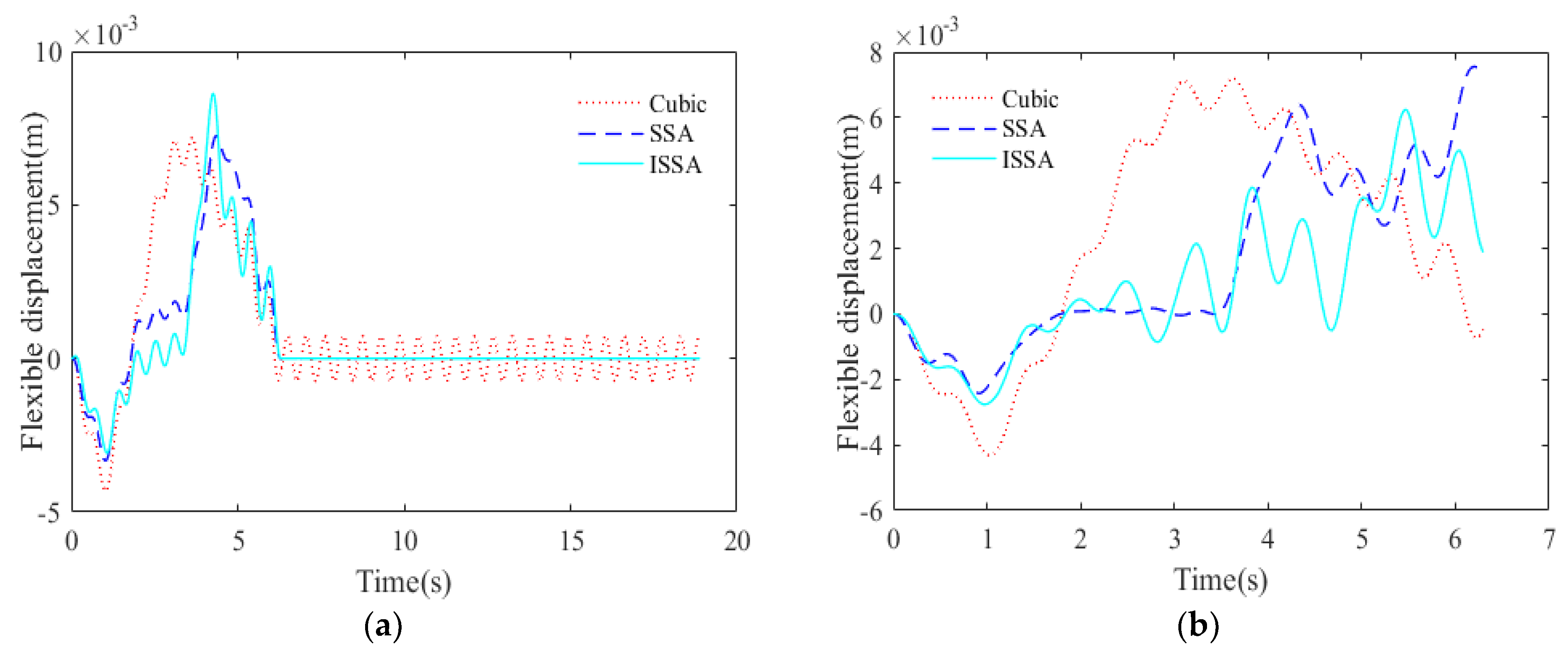
4.4.1. Trajectory Planning with Different Gravity Conditions
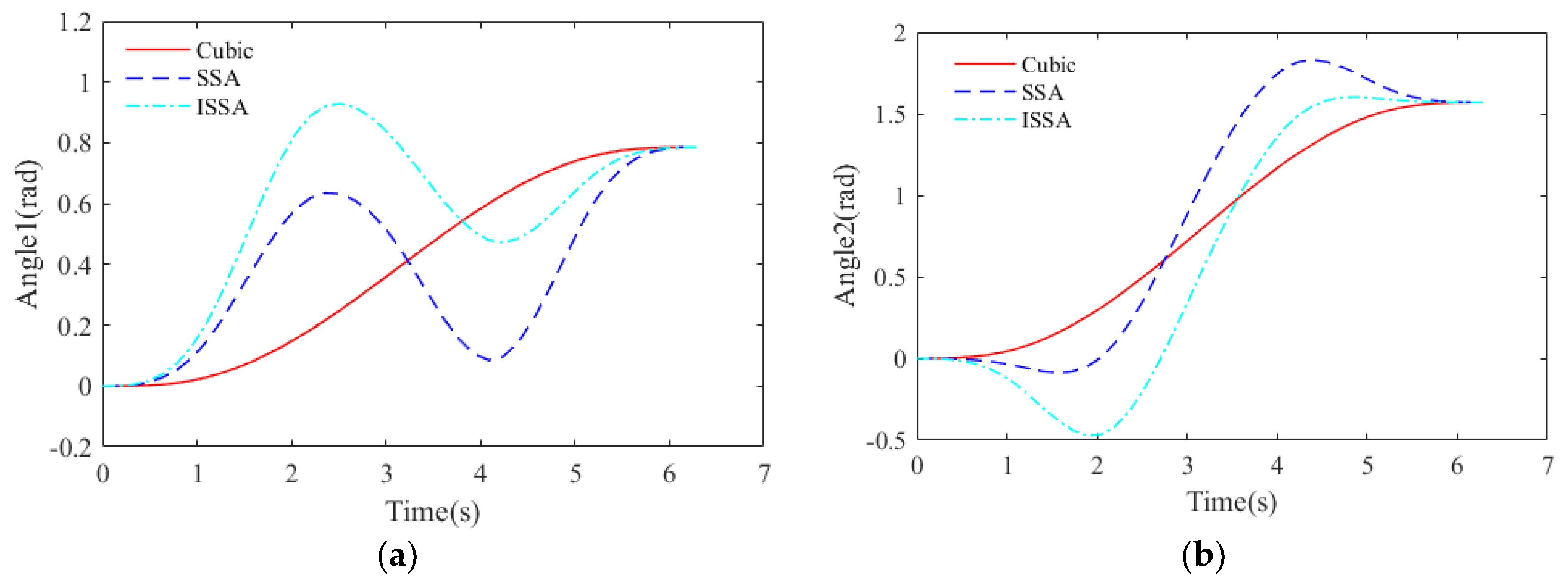
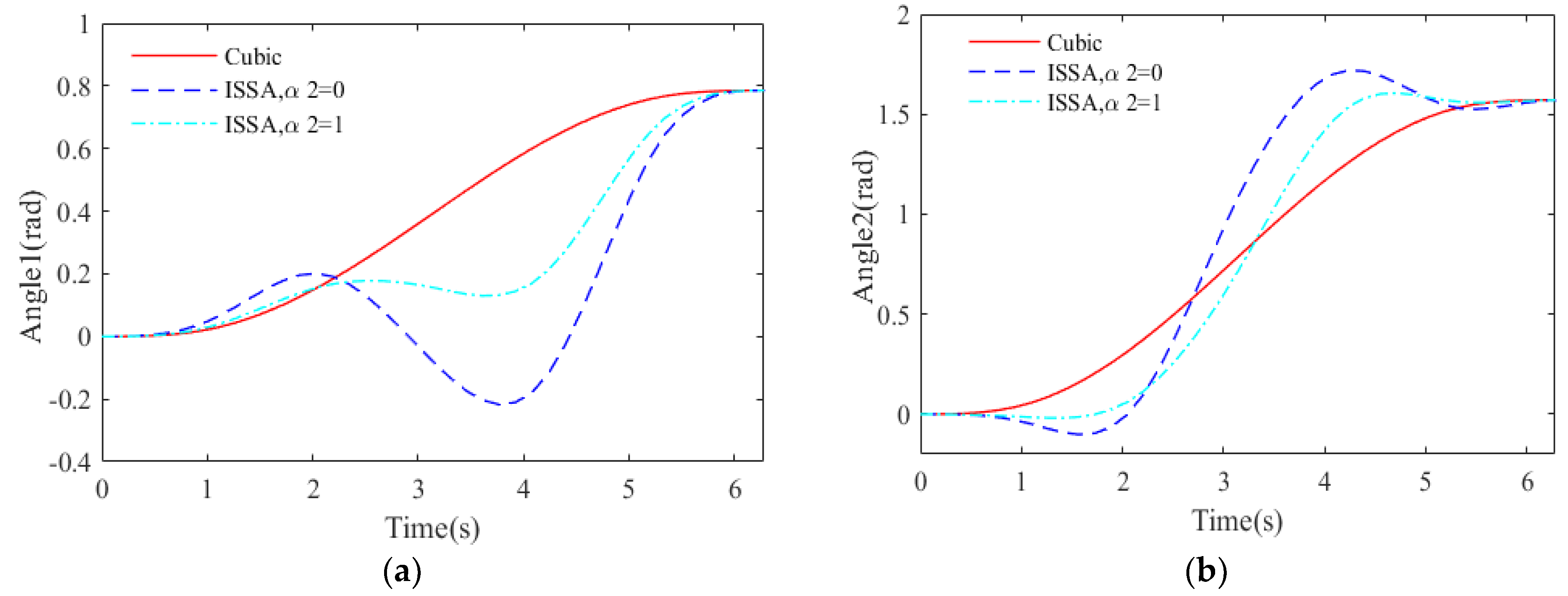
4.4.2. Trajectory Planning with Different Weight Factors
5. Incremental Kriging-Assisted ISSA
5.1. Incremental Learning Kriging Model
5.2. Infill Criteria
| Algorithm 1. Optimization process of IKA-ISSA. |
| Parameters: number of sample points Nt, maximum number of sample points Nm, learning increment step of Kriging model |
| 1. Initial sample set generation: Latin superelevation method to generate N initial design points . the response value of vibration accumulation and the maximum flexible displacement constraint value obtained by the dynamic model. |
| 2. Generate objective function values: generate objective function y with penalty factors based on response and constraint values and rank to obtain the optimal value . |
| 3. While Nt < Nm do |
| 4. If = = 1 |
| Generating the initial Kriging model: the initial sample set is used to generate the responding Kriging model and the constrained Kriging model , respectively. |
| 5. Else |
| Update the Kriging model: generate new Kriging models , based on the Kriging model from the previous learning increment step and the sample set increments , , . |
| End if |
| 6. ISSA optimization: set the optimal population P, obtain the predicted value of the population sample based on the initial Kriging model and perform iterations of ISSA optimization to obtain the optimized population P1. |
| 7. Generate candidate increment set: merge similar individuals in population P1 to generate population P2. Remove points in population P2 that are similar to sample set as candidate increment set . |
| 8. Generate increment sets: select sample set increments , , from the candidate increment set based on MSP + EI infill criterion and Kriging model. |
| 9. Generate objective function values of infill points: obtain the response value and the constraint value for the sample set increment through the dynamic model and calculate the objective function for the increment sample set. |
| 10. Update variables: update the sample sets , , ; update Nt and ; update the optimal value and the corresponding optimal point . |
| 11. End while |
| 12. Output optimal solution: Output and . |
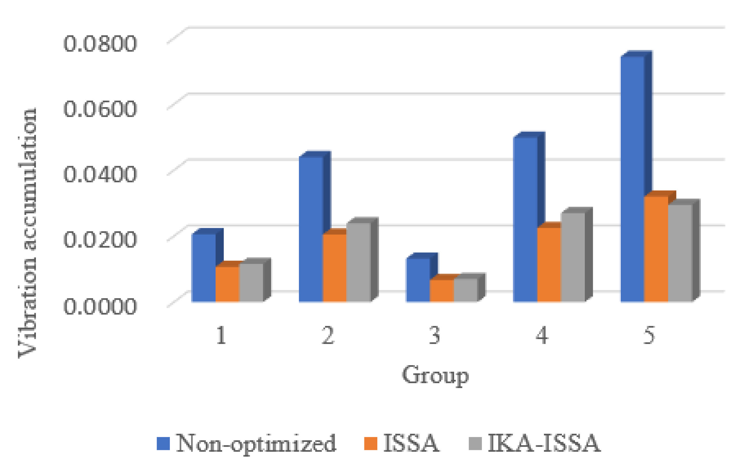
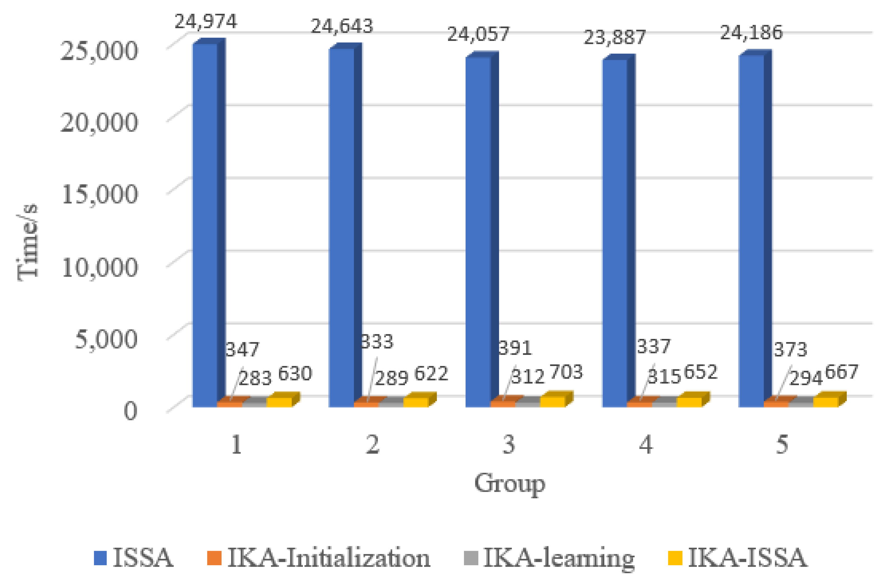
5.3. Simulation
6. Conclusions
Author Contributions
Funding
Institutional Review Board Statement
Informed Consent Statement
Data Availability Statement
Conflicts of Interest
Nomenclature
| SSA | Sparrow search algorithm | Early warning value | |
| ISSA | Improved sparrow search algorithm | Safety value | |
| PSO | Particle swarm optimization | The proportion of early warnings | |
| IKA-ISSA | Incremental Kriging-assisted ISSA | The proportion of discoverers | |
| GA | Genetic algorithm | The proportion of elite groups | |
| UUV | Unmanned underwater vehicles | Sine cosine switching coefficient | |
| AMM | Assumed mode method | Elite group | |
| Joint angle | Optimize iteration steps | ||
| First two-order modes | Learning factor | ||
| Stiffness matrix | Maximum number of iterations | ||
| Centrifugal forces, Coriolis forces and gravity terms | Random number subject to normal distribution | ||
| Mass matrices, represents or | 1 × d-dimensional matrix in which each element is l | ||
| Generalized force related to hydrodynamic force | Best position of the current discoverer | ||
| Joint torque | Worst position in the current global situation | ||
| Reference joint angle trajectory | Global optimal position | ||
| Initial joint angle | Step control parameter | ||
| Joint angle at end time | Number of individuals in the population | ||
| End time | Optimized dimensionality | ||
| Joint angle of the i-th trajectory control point | The number of data points for the fourth-order Runge–Kutta model | ||
| Floating value of the i-th trajectory control point | EI criterion | ||
| Basic value of the i-th trajectory control point | EI criterion with constraints | ||
| Cubic polynomial over the time interval | Objective function | ||
| Angular velocities at the start time and the end time | Hyperparameters | ||
| Angular acceleration at the start time and the end time | Gaussian process with mean zero | ||
| Maximum angular velocity for joint j | Correlation matrix | ||
| Maximum angular acceleration for joint j | Maximum likelihood estimation of hyperparameters | ||
| Flexible displacement at the end of the manipulator | Correlation vector | ||
| First two-order modal shape functions | Lower triangular matrix | ||
| Weight factors | Incremental matrix of new data | ||
| Position of the population | Objective value of sample points | ||
| Velocity of the particle | Best linear unbiased prediction | ||
| Optimal solution of the particle | Error estimation of the prediction | ||
| Global optimal solution currently found | Standard normal cumulative distribution function | ||
| Random number | Standard normal probability density function | ||
| Random number | Incremental form of | ||
| Best individual of the group after the t-th iteration | Updated correlation matrix |
References
- Irani, R.A.; Limited, R.-R.C.; Kehoe, D.; Spencer, W.W.; Watt, G.D.; Gillis, C.; Carretero, J.A.; Dubay, R. Towards a UUV launch and recovery system on a slowly moving submarine. In Proceedings of the International Conference on Warship, Bath, UK, 15–16 June 2014. [Google Scholar]
- Watt, G.D.; Roy, A.R.; Currie, J.; Gillis, C.B.; Giesbrecht, J.; Heard, G.J.; Birsan, M.; Seto, M.L.; Carretero, J.A.; Dubay, R.; et al. A Concept for Docking a UUV With a Slowly Moving Submarine Under Waves. IEEE J. Ocean. Eng. 2015, 41, 471–498. [Google Scholar] [CrossRef]
- Sivčev, S.; Coleman, J.; Omerdić, E.; Dooly, G.; Toal, D. Underwater manipulators: A review. Ocean Eng. 2018, 163, 431–450. [Google Scholar] [CrossRef]
- Vakil, M.; Fotouhi, R.; Nikiforuk, P.N. A new method for dynamic modeling of flexible-link flexible-joint manipulators. J. Vib. Acoust.-Trans. ASME. 2011, 134, 014503. [Google Scholar] [CrossRef]
- Meng, D.; Wang, X.; Xu, W.; Liang, B. Space robots with flexible appendages: Dynamic modeling, coupling measurement, and vibration suppression. J. Sound Vib. 2017, 396, 30–50. [Google Scholar] [CrossRef]
- Sahu, U.K.; Patra, D. Observer based backstepping method for tip tracking control of 2-DOF Serial Flexible Link Manipulator. In Proceedings of the Region 10 Conference, Singapore, 22–25 November 2016. [Google Scholar]
- Yang, Y.-L.; Wei, Y.-D.; Lou, J.-Q.; Fu, L.; Fang, S.; Chen, T.-H. Dynamic modeling and adaptive vibration suppression of a high-speed macro-micro manipulator. J. Sound Vib. 2018, 422, 318–342. [Google Scholar] [CrossRef]
- Rahmani, B.; Belkheiri, M. Adaptive Neural Network Output Feedback Control for Flexible Multi-Link Robotic Manipulators. Int. J. Control. 2018, 92, 2324–2338. [Google Scholar] [CrossRef]
- Yavuz, Ş. An improved vibration control method of a flexible non-uniform shaped manipulator. Simul. Model. Pract. Theory 2021, 111, 102348. [Google Scholar] [CrossRef]
- Guo, Z.; Zhang, J.; Zhang, P. Research on the Residual Vibration Suppression of Delta Robots Based on the Dual-Modal Input Shaping Method. Actuators 2023, 12, 84. [Google Scholar] [CrossRef]
- Xu, S.; Cui, N.; Fan, Y.; Guan, Y. A Study on Optimal Compensation Design for Meteorological Satellites in the Presence of Periodic Disturbance. Appl. Sci. 2018, 8, 1190. [Google Scholar] [CrossRef]
- Sands, T. Optimization Provenance of Whiplash Compensation for Flexible Space Robotics. Aerospace 2019, 6, 93. [Google Scholar] [CrossRef]
- Park, K.-J.; Park, Y.-S. Fourier-based optimal design of a flexible manipulator path to reduce residual vibration of the endpoint. Robotica 1993, 11, 263–272. [Google Scholar] [CrossRef]
- Wu, H.; Sun, F.; Sun, Z.; Wu, L. Optimal Trajectory Planning of a Flexible Dual-Arm Space Robot with Vibration Reduction. J. Intell. Robot. Syst. 2004, 40, 147–163. [Google Scholar] [CrossRef]
- Guo, C.; Gao, H.; Ni, F.; Liu, H. A vibration suppression method for flexible joints manipulator based on trajectory optimization. In Proceedings of the IEEE International Conference on Mechatronics & Automation, Harbin, China, 7–10 August 2016. [Google Scholar] [CrossRef]
- Cui, L.; Wang, H.; Chen, W. Trajectory planning of a spatial flexible manipulator for vibration suppression. Robot. Auton. Syst. 2019, 123, 103316. [Google Scholar] [CrossRef]
- Lin, C.; Chang, P.; Luh, J. Formulation and Optimization of Cubic Polynomial Joint Trajectories for Industrial Robots. IEEE Trans. Autom. Control 1984, 28, 1066–1074. [Google Scholar] [CrossRef]
- Yin, H.; Kobayashi, Y.; Hoshino, Y.; Emaru, T. Hybrid sliding mode control with optimization for flexible manipulator under fast motion. In Proceedings of the Robotics and Automation (ICRA), 2011 IEEE International Conference, Shanghai, China, 9–13 May 2011; pp. 458–463. [Google Scholar] [CrossRef]
- Li, Y.; Ge, S.S.; Wei, Q.; Gan, T.; Tao, X. An Online Trajectory Planning Method of a Flexible-Link Manipulator Aiming at Vibration Suppression. IEEE Access 2020, 8, 130616–130632. [Google Scholar] [CrossRef]
- Yue, H.S.; Henrich, D.; Xu, W.L. Trajectory planning in joint space for flexible robots with kinematics redundancy. In Proceedings of the IASTED International Conference, Honolulu, HI, USA, 13–16 August 2001; pp. 1–6. [Google Scholar]
- Kazem, I.B.; Mahdi, A.I.; Oudah, A.T. Motion Planning for a Robot Arm by Using Genetic Algorithm. Jordan J. Mech. Ind. Eng. 2008, 2, 131–136. [Google Scholar]
- Qingmei, L.; Jia, J.; Yu-An, H. Vibration suppression of manipulator using quantum genetic algorithm. In Proceedings of the Information Technology, Networking, Electronic and Automation Control, Chengdu, China, 15–17 December 2017; pp. 802–807. [Google Scholar] [CrossRef]
- Kramer, O. A Review of Constraint-Handling Techniques for Evolution Strategies. Appl. Comput. Intell. Soft Comput. 2010, 2010, 185063. [Google Scholar] [CrossRef]
- Jordehi, A.R. A review on constraint handling strategies in particle swarm optimisation. Neural Comput. Appl. 2015, 26, 1265–1275. [Google Scholar] [CrossRef]
- Kohler, M.; Forero, L.; Vellasco, M.; Tanscheit, R.; Pacheco, M.A. PSO+: A nonlinear constraints-handling particle swarm optimization. In Proceedings of the IEEE Congress on Evolutionary Computation (CEC), Vancouver, BC, Canada, 24–29 July 2016; pp. 2518–2523. [Google Scholar] [CrossRef]
- Cao, B.; Sun, K.; Li, T.; Gu, Y.; Jin, M.; Liu, H. Trajectory Modified in Joint Space for Vibration Suppression of Manipulator. IEEE Access 2018, 6, 57969–57980. [Google Scholar] [CrossRef]
- Wang, M.; Luo, J.; Yuan, J.; Walter, U. Coordinated trajectory planning of dual-arm space robot using constrained particle swarm optimization. Acta Astronaut. 2018, 146, 259–272. [Google Scholar] [CrossRef]
- Xue, J.; Shen, B. A novel swarm intelligence optimization approach: Sparrow search algorithm. Syst. Sci. Control. Eng. 2020, 8, 22–34. [Google Scholar] [CrossRef]
- Zhang, Z.; He, R.; Yang, K. A bioinspired path planning approach for mobile robots based on improved sparrow search algorithm. Adv. Manuf. 2022, 10, 114–130. [Google Scholar] [CrossRef]
- Liu, G.; Shu, C.; Liang, Z.; Peng, B.; Cheng, L. A Modified Sparrow Search Algorithm with Application in 3d Route Planning for UAV. Sensors 2021, 21, 1224. [Google Scholar] [CrossRef]
- Farivarnejad, H.; Moosavian, S.A.A. Multiple Impedance Control for object manipulation by a dual arm underwater vehicle–manipulator system. Ocean Eng. 2014, 89, 82–98. [Google Scholar] [CrossRef]
- Li, J.; Huang, H.; Wan, L.; Zhou, Z.; Xu, Y. Hybrid Strategy-based Coordinate Controller for an Underwater Vehicle Manipulator System Using Nonlinear Disturbance Observer. Robotica 2019, 37, 1710–1731. [Google Scholar] [CrossRef]
- Huang, H.; Tang, G.Y.; Han, L.J.; Cheng, M.L.; Xie, D.; Chen, H.X. Neural network Adaptive Backstepping Control of Multi-link Underwater Flexible Manipulators. In Proceedings of the 31st International Ocean and Polar Engineering Conference, Rhodes, Greece, 20–25 June 2021. [Google Scholar]
- Huang, H.; Tang, G.; Chen, H.; Han, L.; Xie, D. Dynamic Modeling and Vibration Suppression for Two-Link Underwater Flexible Manipulators. IEEE Access 2022, 10, 40181–40196. [Google Scholar] [CrossRef]
- Kennedy, J.; Eberhart, R. Particle Swarm Optimization. In Proceedings of the ICNN’95—International Conference on Neural Networks, Perth, Australia, 27 November–1 December 1995; pp. 1942–1948. [Google Scholar] [CrossRef]
- Clerc, M.; Kennedy, J. The particle swarm—Explosion, stability, and convergence in a multidimensional complex space. IEEE Trans. Evol. Comput. 2002, 6, 58–73. [Google Scholar] [CrossRef]
- Mirjalili, S. SCA: A Sine Cosine Algorithm for solving optimization problems. Knowl.-Based Syst. 2016, 96, 120–133. [Google Scholar] [CrossRef]
- Tizhoosh, H. Opposition-based learning: A new scheme for machine intelligence. In Proceedings of the International Conference on Computational Intelligence for Modelling, Control and Automation, Vienna, Austria, 28–30 November 2005; pp. 695–701. [Google Scholar] [CrossRef]
- Zhao, C.; Dinar, M.; Melkote, S.N. A data-driven framework for learning the capability of manufacturing process sequences. J. Manuf. Syst. 2022, 64, 68–80. [Google Scholar] [CrossRef]
- Zhang, S.; Liang, P.; Pang, Y.; Li, J.; Song, X. Multi-fidelity surrogate model ensemble based on feasible intervals. Struct. Multidiscip. Optim. 2022, 65, 1–13. [Google Scholar] [CrossRef]
- Yang, Z.; Pak, U.; Yan, Y.; Kwon, C. Reliability-based robust optimization design for vehicle drum brake considering multiple failure modes. Struct. Multidiscip. Optim. 2022, 65, 1–17. [Google Scholar] [CrossRef]
- Zhan, D.; Xing, H. A fast kriging-assisted evolutionary algorithm based on incremental learning. IEEE Trans. Evol. Comput. 2021, 25, 941–955. [Google Scholar] [CrossRef]
- Zhong, J.; Zheng, Y.; Chen, J.; Jing, Z. Variable-stiffness composite cylinder design under combined loadings by using the improved Kriging model. Acta Mech. Sin. 2019, 35, 201–211. [Google Scholar] [CrossRef]


| Parameter | Symbol | Value |
|---|---|---|
| Length (m) | ||
| Density (kg·m−1) | ||
| Bending stiffness (N·m2) | 125 | |
| Water resistance coefficient | 1.1 | |
| Additional mass coefficient | 1 |
| Case | Algorithm | Optimization Algorithm Parameters |
|---|---|---|
| Case 1 (without gravity) | PSO | N = 30, d = 6, c1 = 2.05, c2 = 2.05, K = 150, , Num = 500 |
| SSA | N = 30, d = 6, ST = 0.7, PD = 0.7, SD = 0.2, K = 150, Num = 500 | |
| OBLSSA | N = 30, d = 6, ST = 0.7, PD = 0.7, SD = 0.2, ED = 0.2, K = 150, Num = 500 | |
| ISSA | N = 30, d = 6, ST = 0.7, PD = 0.7, SD = 0.2, ED = 0.2, = 2, K = 150, Num = 500 | |
| Case 1 (with gravity) | PSO | N = 30, d = 6, c1 = 2.05, c2 = 2.05, K = 150, , Num = 500 |
| SSA | N = 30, d = 6, ST = 0.7, PD = 0.7, SD = 0.2, K = 150, Num = 500 | |
| OBLSSA | N = 30, d = 6, ST = 0.7, PD = 0.7, SD = 0.2, ED = 0.2, K = 150, Num = 500 | |
| ISSA | N = 30, d = 6, ST = 0.7, PD = 0.7, SD = 0.2, ED = 0.2, = 2, K = 150, Num = 500 | |
| Case 2 () | PSO | N = 30, d = 8, c1 = 2.05, c2 = 2.05, K = 150, , Num = 500 |
| SSA | N = 30, d = 8, ST = 0.7, PD = 0.7, SD = 0.2, K = 150, Num = 500 | |
| OBLSSA | N = 30, d = 8, ST = 0.7, PD = 0.7, SD = 0.2, ED = 0.2, K = 150, Num = 500 | |
| ISSA | N = 30, d = 8, ST = 0.7, PD = 0.7, SD = 0.2, ED = 0.2, = 2, K = 150, Num = 500 | |
| Case 2 () | PSO | N = 30, d = 8, c1 = 2.05, c2 = 2.05, K = 150, , Num = 500 |
| SSA | N = 30, d = 8, ST = 0.7, PD = 0.7, SD = 0.2, K = 150, Num = 500 | |
| OBLSSA | N = 30, d = 8, ST = 0.7, PD = 0.7, SD = 0.2, ED = 0.2, K = 150, Num = 500 | |
| ISSA | N = 30, d = 8, ST = 0.7, PD = 0.7, SD = 0.2, ED = 0.2, = 2, K = 150, Num = 500 |
| Case | Algorithm | Optimal Solution | Running Time/s | ||
|---|---|---|---|---|---|
| Best | Worst | Mean | |||
| Case 1 (without gravity) | PSO | 0.0096 | 0.0111 | 0.0101 | 66,838 |
| SSA | 0.0162 | 0.0166 | 0.0163 | 16,434 | |
| OBLSSA | 0.0108 | 0.0121 | 0.0110 | 19,978 | |
| ISSA | 0.0095 | 0.0095 | 0.0095 | 17,518 | |
| Case 1 (with gravity) | PSO | 0.0622 | 0.0622 | 0.0622 | 65,619 |
| SSA | 0.0617 | 0.0617 | 0.0617 | 19,058 | |
| OBLSSA | 0.0630 | 0.0632 | 0.0631 | 22,286 | |
| ISSA | 0.0608 | 0.0612 | 0.0609 | 18,673 | |
| Case 2 () | PSO | 0.0191 | 0.0191 | 0.0191 | 67,459 |
| SSA | 0.0174 | 0.0174 | 0.0174 | 16,893 | |
| OBLSSA | 0.0206 | 0.0208 | 0.0207 | 20,974 | |
| ISSA | 0.0148 | 0.0148 | 0.0148 | 18,146 | |
| Case 2 () | PSO | 0.0217 | 0.0217 | 0.0217 | 82,930 |
| SSA | 0.0137 | 0.0145 | 0.0142 | 15,743 | |
| OBLSSA | 0.0132 | 0.0135 | 0.0133 | 19,876 | |
| ISSA | 0.0112 | 0.0113 | 0.0113 | 22,495 | |
| Optimization Algorithm | ||
|---|---|---|
| PSO | 25.0% | 3.68 |
| SSA | 29.2% | 0.90 |
| OBLSSA | 32.6% | 1.10 |
| ISSA | 42.3% | 1.00 |
Disclaimer/Publisher’s Note: The statements, opinions and data contained in all publications are solely those of the individual author(s) and contributor(s) and not of MDPI and/or the editor(s). MDPI and/or the editor(s) disclaim responsibility for any injury to people or property resulting from any ideas, methods, instructions or products referred to in the content. |
© 2023 by the authors. Licensee MDPI, Basel, Switzerland. This article is an open access article distributed under the terms and conditions of the Creative Commons Attribution (CC BY) license (https://creativecommons.org/licenses/by/4.0/).
Share and Cite
Huang, H.; Tang, G.; Chen, H.; Wang, J.; Han, L.; Xie, D. Vibration Suppression Trajectory Planning of Underwater Flexible Manipulators Based on Incremental Kriging-Assisted Optimization Algorithm. J. Mar. Sci. Eng. 2023, 11, 938. https://doi.org/10.3390/jmse11050938
Huang H, Tang G, Chen H, Wang J, Han L, Xie D. Vibration Suppression Trajectory Planning of Underwater Flexible Manipulators Based on Incremental Kriging-Assisted Optimization Algorithm. Journal of Marine Science and Engineering. 2023; 11(5):938. https://doi.org/10.3390/jmse11050938
Chicago/Turabian StyleHuang, Hui, Guoyuan Tang, Hongxuan Chen, Jianjun Wang, Lijun Han, and De Xie. 2023. "Vibration Suppression Trajectory Planning of Underwater Flexible Manipulators Based on Incremental Kriging-Assisted Optimization Algorithm" Journal of Marine Science and Engineering 11, no. 5: 938. https://doi.org/10.3390/jmse11050938