

New Insights into the Seamount Structure of the Northern Part of the Ninetyeast Ridge (Indian Ocean) through the Integrated Analysis of Geophysical Data
 ,
, 
Abstract
:1. Introduction
2. Methods and Results
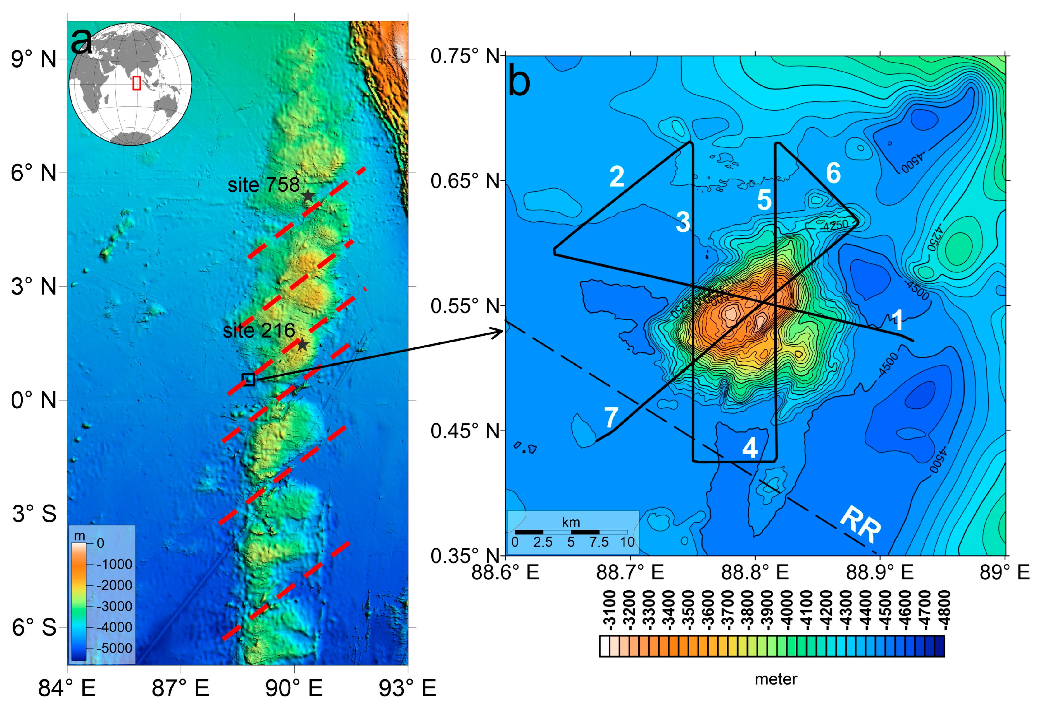
2.1. Bathymetry
2.1.1. Methods
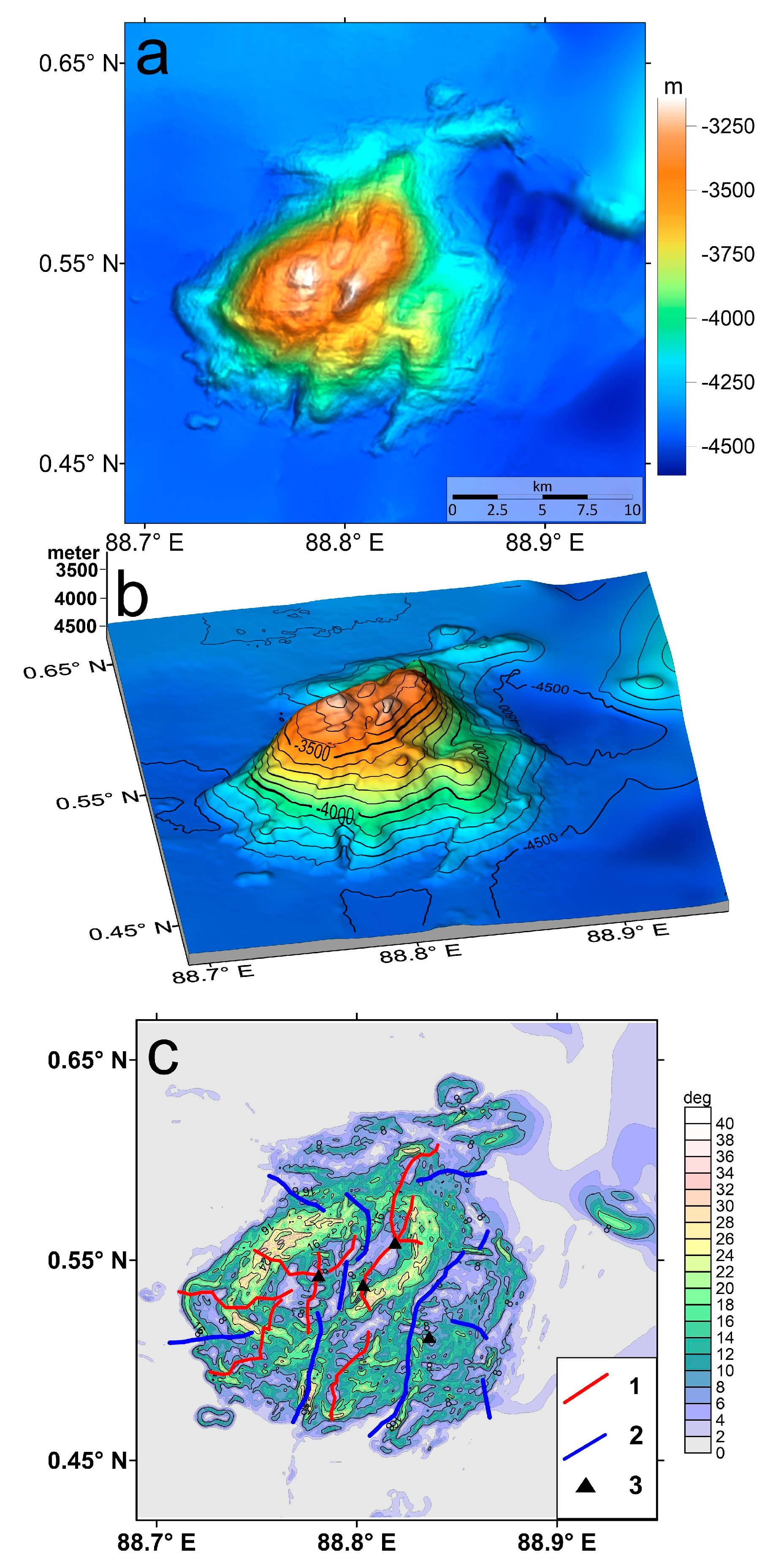
2.1.2. Results
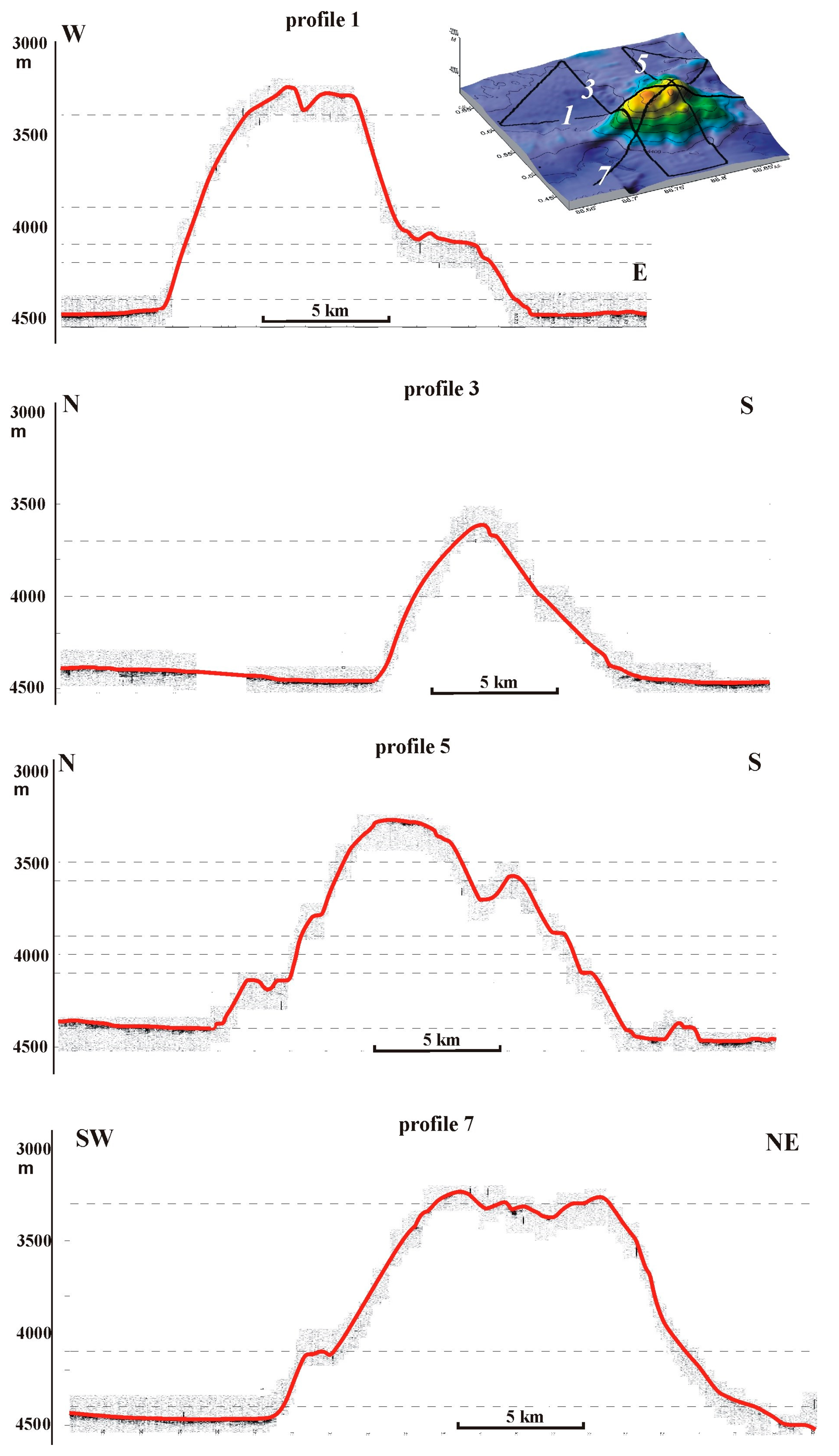
2.2. Seismic Profiling
2.2.1. Methods
2.2.2. Results
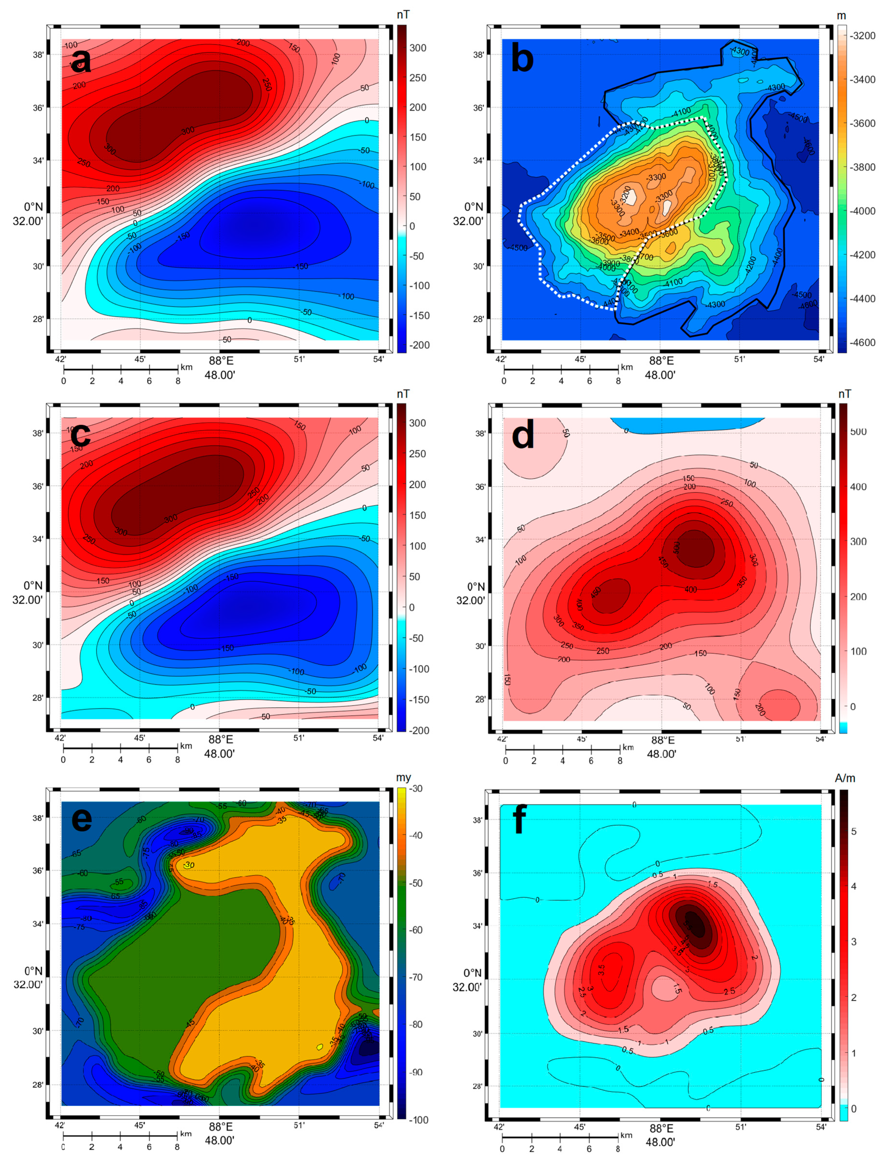
2.3. Magnetic Survey
2.3.1. Data and Methods
2.3.2. Results
3. Discussion
4. Conclusions
- (1)
- The studied seamount appears to consist of two different-age fragments formed about 47 Ma and 23 Ma, respectively, 31 and 55 Ma after the main Ninetyeast Ridge massif. In the first stage, the main western part of the seamount was formed. Then, during the exploratory phase of magmatic activity, the volcanic structure expanded eastward;
- (2)
- The explored seamount located at latitude 0.5° N and the volcano of the late Miocene age located to the south at latitude 10° S [16] are in the zone of one of the giant meridional faults that define the NER fault structure [8]. It is likely that the mechanism of formation of these two volcanic structures is somewhat the same, although the timing of formation differs significantly. As for the two volcanoes on the NER dome near 17° S [19], these appeared to be related to the underplating magmatism of the reactivation of this fault when the critical intraplate compression during continental collision was reached;
- (3)
- The morphology of the studied seamount suggests that it was formed as a result of magma outpourings in the SW-NE strike-slip fault after the formation of the main NER massif in the zone of a giant meridional fault [24]. Presumably, these SW-NE strike-slip faults are second-order structures that apparently formed in the zone of the ancient meridional transform fault [12]. The process was complicated by the fact that shear deformations occurred along the fault during the relaxation of excess regional compression stress with a NW-SE vector in the body of the Indo-Australian lithospheric plate due to continental collision at its northern boundary. These shifts potentially created the local tensile fault zones necessary for this, along which the rise of magmatic material took place;
- (4)
- The results of comprehensive studies performed in cruise #42 of the R/V Akademik Boris Petrov suggest rather long cyclic magmatic activity in the northern segment of the NER after 47 Ma already after the formation of its main massif at about 80 Ma.
Author Contributions
Funding
Institutional Review Board Statement
Informed Consent Statement
Data Availability Statement
Acknowledgments
Conflicts of Interest
References
- Koppers, A.A.P.; Watts, A.B. Intraplate seamounts as a window into deep earth processes. Oceanography 2010, 23, 42–57. [Google Scholar] [CrossRef]
- Hedervari, P.A. Possible submarine volcano near the central part of Ninety-East Ridge, Indian Ocean. J. Volcanol. Geotherm. Res. 1982, 13, 199–211. [Google Scholar] [CrossRef]
- Mukhopadhyay, R.; Batiza, R. Basinal Seamounts and Seamount Chains of the Central Indian Ocean: Probable Near-Axis Origin from a Fast-Spreading Ridge. Mar. Geoph. Res. 1994, 16, 303–314. [Google Scholar] [CrossRef]
- Mukhopadhyay, R. Post-Cretaceous intraplate volcanism in the Central Indian Basin. Mar. Geol. 1998, 151, 135–142. [Google Scholar] [CrossRef]
- Das, P.; Iyer, S.D.; Kodagali, V.N.; Krishna, K.S. Distribution and Origin of Seamounts in the Central Indian Ocean Basin. Mar. Geod. 2005, 28, 259–269. [Google Scholar] [CrossRef]
- Iyer, S.D.; Das, P.; Kalangutkar, N.G. Seamounts—Windows of opportunities and the Indian scenario. Curr. Sci. 2012, 102, 1382–1391. [Google Scholar]
- Homrighausen, S.; Hoernle, K.; Wartho, J.-A.; Hauff, F.; Werner, R. Do the 85° E Ridge and Conrad Rise form a hotspot track crossing the Indian Ocean? Lithos 2021, 398–399, 106234. [Google Scholar] [CrossRef]
- Royer, J.-Y.; Peirce, J.W.; Weissel, J.K. Tectonic constraints on the hot-spot formation of Ninetyeast Ridge. Proc. ODP Sci. Res. 1991, 121, 763–776. [Google Scholar] [CrossRef]
- Krishna, K.S.; Abraham, H.; Sager, W.W. Tectonics of the Ninetyeast Ridge derived from spreading records in adjacent ocean basins and age constraints of the ridge. J. Geophys. Res. 2012, 117, B04101. [Google Scholar] [CrossRef]
- Nobre Silva, G.; Weis, D.; Scoates, J.S.; Barling, J. The Ninetyeast Ridge and its relation to the Kerguelen, Amsterdam and St. Paul Hotspots in the Indian ocean. J. Petrol. 2013, 54, 1177–1210. [Google Scholar] [CrossRef]
- Frey, F.A.; Silva, I.G.N.; Huang, S.; Pringle, M.S.; Meleney, P.R.; Weis, D. Depleted components in the source of hotspot magmas: Evidence from the Ninetyeast Ridge (Kerguelen). Earth Planet. Sci. Let. 2015, 426, 293–304. [Google Scholar] [CrossRef]
- Sushchevskaya, N.M.; Levchenko, O.V.; Dubinin, E.P.; Belyatsky, B.V. Ninetyeast Ridge: Magmatism and geodynamics. Geochem. Int. 2016, 54, 237–256. [Google Scholar] [CrossRef]
- Levchenko, O.V.; Sushchevskaya, N.M.; Marinova, Y.G. The Nature and Evolution of the Ninetyeast Ridge: A Key Tectonic and Magmatic Feature of the East Indian Ocean. Geotectonics 2021, 55, 194–218. [Google Scholar] [CrossRef]
- Von der Borch, C.C.; Christopher, C.; Sclater, J.G.; Veevers, J.J.; Hekinian, R.; Thompson, R.W.; Pimm, A.C.; McGowran, B.; Gartner, S., Jr.; Johnson, D.A. Initial Reports of the Deep-Sea Drilling Project; US Government Printing Office: Washington, DC, USA, 1974; Volume 22, p. 890.
- Weissel, J.; Peirce, J.; Taylor, E.; Alt, J. Proceedings of the ODP: Scientific Results; Ocean Drilling Program: College Station, TX, USA, 1991; Volume 121, p. 990. [Google Scholar]
- Kumar, R.T.; Windley, B.F. Spatial variations of effective elastic thickness over the Ninetyeast Ridge and implications for its structure and tectonic evolution. Tectonophysics 2013, 608, 847–856. [Google Scholar] [CrossRef]
- Sreejith, K.M.; Krishna, K.S. Magma production rate along the Ninetyeast Ridge and its relationship to Indian Plate motion and Kerguelen Hot Spot activity. Geophys. Rev. Lett. 2015, 42, 1105–1112. [Google Scholar] [CrossRef]
- Evsyukov, Y.D. Morphology of the Ninetyeast Ridge north of the equator. Oceanology 2003, 43, 270–275. [Google Scholar]
- Kopf, A.; Klaeschen, D.; Weinrebe, W.; Flueh, E.R.; Grevemeyer, I. Geophysical evidence for late stage magmatism at the central Ninetyeast ridge, Eastern Indian Ocean. Mar. Geophys. Res. 2001, 22, 225–234. [Google Scholar] [CrossRef]
- Sager, W.W.; Bull, J.M.; Krishna, K.S. Active faulting on the Ninetyeast Ridge and its relation to deformation of the Indo-Australian plate. J. Geophys. Res. 2013, 118, 13755–13782. [Google Scholar] [CrossRef]
- Levchenko, O.V.; Sborshchikov, I.M.; Marinova, Y.G. Tectonics of the Ninetyeast Ridge. Oceanology 2014, 54, 231–244. [Google Scholar] [CrossRef]
- Kashintsev, G.L.; Levchenko, O.V. Miocene volcanism of the Ninetyeast Ridge. Dokl. Earth Sci. 2009, 428, 1054–1057. [Google Scholar] [CrossRef]
- Bezrukov, P.I.; Neprochnov, Y.P. (Eds.) Geology and Geophysics of the Sea Floor in the Eastern Indian Ocean; Nauka: Moskow, Russia, 1981; 255p. (In Russian) [Google Scholar]
- Kashintsev, G.L. Aspects of magmatism of the Ninetyeast Ridge. Oceanology 2001, 41, 413–418. [Google Scholar]
- Levchenko, O.V.; Shapovalov, S.M. Return of Russian Oceanographers to the Indian Ocean: Multidisciplinary Study during the 42nd Cruise of the Research Vessel Akademik Boris Petrov. Oceanology 2019, 59, 164–167. [Google Scholar] [CrossRef]
- GEBCO (General Bahtymetric Chart of the Oceans). The GEBCO_2019 Grid. Available online: https://www.gebco.net/data_and_products/gridded_bathymetry_data/ (accessed on 10 December 2022).
- Multibeam Report for RR1510. Ship Name: Roger Revelle: Chief Scientist: None: Source Organization: UNOLS R2R: Start Date: 8 July 2015: End Date: 2 August 2015. Available online: https://www.ngdc.noaa.gov/ships/roger_revelle/RR1510_mb.html (accessed on 15 December 2022).
- Stein, S.; Okal, E.O. Seismicity and tectonics of the Ninetyeast Ridge area: Evidence for internal deformation of the Indian plate. J. Geophys. Res. 1978, 83, 2233–2246. [Google Scholar] [CrossRef]
- Petroy, D.E.; Wiens, D.A. Historical seicmicity and implications for diffuse plate convergence in the northeast Indian Ocean. J. Geophys. Res. 1989, 94, 12301–12319. [Google Scholar] [CrossRef]
- Bastia, R.; Radhakrishna, M.; Das, S.; Kale, A.S.; Catuneanu, O. Delineation of the 85° E ridge and its structure in the Mahanadi Offshore Basin, Eastern Continental Margin of India (ECMI), from seismic reflection imaging. Mar. Pet. Geol. 2010, 27, 1841–1848. [Google Scholar] [CrossRef]
- Satriano, C.; Kiraly, E.; Pascal Bernard, P.; Vilotte, J.-P. The 2012 Mw 8.6 Sumatra earthquake: Evidence of westward sequential seismic ruptures associated to the reactivation of a N-S ocean fabric. Geophys. Res. Lett. 2012, 39, L15302. [Google Scholar] [CrossRef]
- Caress, D.W.; Chayes, D.N. MB-System Version 5.5.2252. Open Source Software Distributed from the MBARI and L-DEO Web Sites, 2000–2015. 2015. Available online: https://www.mbari.org/products/research-software/mb-system/ (accessed on 20 November 2022).
- GEODAS. Available online: https://www.ncei.noaa.gov/maps/bathymetry/ (accessed on 20 November 2022).
- Conrad, O.; Bechtel, B.; Bock, M.; Dietrich, H.; Fischer, E.; Gerlitz, L.; Wehberg, J.; Wichmann, V.; Böhner, J. System for Automated Geoscientific Analyses (SAGA) v. 2.1.4. Geosci. Model Dev. 2015, 8, 1991–2007. [Google Scholar] [CrossRef]
- Catuneanu, O. Principles of Sequence Stratigraphy, 2nd ed.; Elsevier: Amsterdam, The Netherlands, 2022; 375p. [Google Scholar]
- Mitchum, R.M. Seismic stratigraphy and global changes of sea level, Part 11: Glossary of terms used in seismic stratigraphy. In Seismic Stratigraphy—Applications to Hydrocarbon Exploration; Payton, C.E., Ed.; AAPG Memoir 26: Tulsa, OK, USA, 1977; pp. 205–212. [Google Scholar]
- Vail, P.R.; Mitchum, R.M.; Todd, R.G.; Widmier, J.M.; Thompsom, S.; Sangree, J.B.; Bubb, J.N.; Hailelid, W.G. Seismic stratigraphy and global changes in sea level. In Seismic Stratigraphy—Applications to Hydrocarbon Exploration; Payton, C.E., Ed.; AAPG Memoir 26: Tulsa, OK, USA, 1977; pp. 49–212. [Google Scholar]
- Clemens, S.C.; Kuhnt, W.; LeVay, L.J.; Anand, P.; Ando, T.; Bartol, M.; Bolton, C.T.; Ding, X.; Gariboldi, K.; Giosan, L.; et al. Indian Monsoon Rainfall. In Proceedings of the International Ocean Discovery Program, College Station, TX, USA, 29 November 2014–29 January 2015; International Ocean Discovery Program: College Station, TX, USA, 2016; Volume 353. [Google Scholar] [CrossRef]
- Lewis, K.W. Slumping on a continental slope inclined at 1°–4°. Sedimentology 1971, 16, 97–110. [Google Scholar] [CrossRef]
- National Centers for Environmental Information, NCEI Database. NGDC. Available online: https://www.ngdc.noaa.gov/mgg/trk/trackline (accessed on 15 December 2022).
- Okubo, Y.; Matsunaga, T. Curie point depth in northeast Japan and its correlation with regional thermal structure and seismicity. J. Geophys. Res. Solid Earth 1994, 99, 22363–22371. [Google Scholar] [CrossRef]
- Thébault, E. Magnetic Anomalies, Interpretation. In Encyclopedia of Solid Earth Geophysics. Encyclopedia of Earth Sciences Series; Gupta, H.K., Ed.; Springer: Dordrecht, The Netherlands, 2011. [Google Scholar] [CrossRef]
- Vine, F.J.; Matthew, D.H. Magnetic anomalies over oceanic ridges. Nature 1963, 199, 947–949. [Google Scholar] [CrossRef]
- Hulot, G.; Olsen, N.; Sabaka, T.J. The Present Field, Chap. 6, Vol. 5. In Geomagnetism; Kono, M., Ed.; Treatise on Geophysics; Elsevier: Amsterdam, The Netherlands, 2007; pp. 33–72. [Google Scholar]
- Baranov, V. Potential Fields and Their Transformations in Applied Geophysics; Borntraeger: Berlin, Germany, 1975; ISBN 3443130089. [Google Scholar]
- Helbig, K. Some integrals of magnetic anomalies and their relationship to the parameters of disturbing body. Z. Geophys. 1962, 29, 83–97. [Google Scholar]
- Caratori Tontini, F.; Pedersen, L.B. Interpreting magnetic data by integral moments. Geophys. J. Int. 2008, 174, 815–824. [Google Scholar] [CrossRef]
- Valyashko, G.M.; Ivanenko, A.N.; Czerniawski, G.E.; Lukyanov, S.V. Interpretation Procedure of Marine Magnetic Data: Topical Problems. In Anomalous Magnetic Field of the World Ocean; Gorodnitsky, A.M., Ed.; CRC Press: Boca Raton, FL, USA, 1995; pp. 21–66. [Google Scholar]
- Spector, A.; Grant, F.S. Statistical models for interpreting aeromagnetic data. Geophysics 1970, 35, 293–302. [Google Scholar] [CrossRef]
- Kelemework, Y.; Fedi, M.; Milano, M. A review of spectral analysis of magnetic data for depth estimation. Geophysics 2021, 86, J33–J58. [Google Scholar] [CrossRef]
- Van Hinsbergen, D.J.J.; de Groot, L.V.; van Schaik, S.J.; Spakman, W.; Bijl, P.K.; Sluijs, A.; Langereis, C.G.; Brinkhuis, H. A Paleolatitude Calculator for Paleoclimate Studies (model version 2.1). PLoS ONE 2015, 10, e0126946. [Google Scholar] [CrossRef]
- Levchenko, O.V.; Milanovsky, V.E.; Popov, A.A. Sediment thickness map and tectonics of the Distal Bengal Fan. Oceanology 1993, 33, 269–275. [Google Scholar]
- Ogg, J. Geomagnetic Polarity Time Scale. In Geologic Time Scale, 1st ed.; Elsevier: Amsterdam, The Netherlands, 2022; pp. 159–192. [Google Scholar] [CrossRef]
- Coffin, M.F. Emplacement and subsidence of Indian Ocean Plateaus and submarine ridges. In Synthesis of Results from Scientific Drilling in the Indian Ocean; Monograph 70; American Geophysical Union: Washington, DC, USA, 1992; pp. 115–125. [Google Scholar]
- Ninkovich, D. Distribution, age and chemical composition of tephra layers in deep-sea sediments of western Indonesia. J. Volcanol. Geotherm. Res. 1979, 5, 67–86. [Google Scholar] [CrossRef]
- Krishna, K.S.; Bull, J.M.; Ishizuka, O.; Scrutton, R.A.; Jaishankar, S.; Banakar, V.K. Growth of the Afanasy Nikitin seamount and its relationship with the 85° E Ridge, northeastern Indian Ocean. J. Earth Syst. Sci. 2014, 123, 33–47. [Google Scholar] [CrossRef]


Disclaimer/Publisher’s Note: The statements, opinions and data contained in all publications are solely those of the individual author(s) and contributor(s) and not of MDPI and/or the editor(s). MDPI and/or the editor(s) disclaim responsibility for any injury to people or property resulting from any ideas, methods, instructions or products referred to in the content. |
© 2023 by the authors. Licensee MDPI, Basel, Switzerland. This article is an open access article distributed under the terms and conditions of the Creative Commons Attribution (CC BY) license (https://creativecommons.org/licenses/by/4.0/).
Share and Cite
Yutsis, V.; Levchenko, O.; Ivanenko, A.; Veklich, I.; Turko, N.; Marinova, Y. New Insights into the Seamount Structure of the Northern Part of the Ninetyeast Ridge (Indian Ocean) through the Integrated Analysis of Geophysical Data. J. Mar. Sci. Eng. 2023, 11, 924. https://doi.org/10.3390/jmse11050924
Yutsis V, Levchenko O, Ivanenko A, Veklich I, Turko N, Marinova Y. New Insights into the Seamount Structure of the Northern Part of the Ninetyeast Ridge (Indian Ocean) through the Integrated Analysis of Geophysical Data. Journal of Marine Science and Engineering. 2023; 11(5):924. https://doi.org/10.3390/jmse11050924
Chicago/Turabian StyleYutsis, Vsevolod, Oleg Levchenko, Alexander Ivanenko, Ilya Veklich, Nataliya Turko, and Yulia Marinova. 2023. "New Insights into the Seamount Structure of the Northern Part of the Ninetyeast Ridge (Indian Ocean) through the Integrated Analysis of Geophysical Data" Journal of Marine Science and Engineering 11, no. 5: 924. https://doi.org/10.3390/jmse11050924