Author Contributions
Conceptualization, M.H. and R.C.E.; Methodology, M.H. and R.C.E.; Software, J.L., M.H. and R.C.E.; Validation, J.L. and M.H.; Formal analysis, J.L.; Investigation, J.L. and M.H.; Resources, M.H.; Writing—original draft, J.L.; Writing—review & editing, M.H. and R.C.E.; Visualization, J.L.; Supervision, M.H. and R.C.E.; Project administration, M.H. All authors have read and agreed to the published version of the manuscript.
Figure 1.
Schematic of the NS computational domain used in this study. Solitary and cnoidal waves are created at the generation zone, using different theories.
Figure 1.
Schematic of the NS computational domain used in this study. Solitary and cnoidal waves are created at the generation zone, using different theories.
Figure 2.
Comparisons of steady-state surface elevations of a solitary wave with , generated by various theories.
Figure 2.
Comparisons of steady-state surface elevations of a solitary wave with , generated by various theories.
Figure 3.
Comparisons of steady-state surface elevation of cnoidal waves generated by various theories. .
Figure 3.
Comparisons of steady-state surface elevation of cnoidal waves generated by various theories. .
Figure 4.
Comparisons of steady-state horizontal particle velocity of cnoidal waves generated by various theories. .
Figure 4.
Comparisons of steady-state horizontal particle velocity of cnoidal waves generated by various theories. .
Figure 5.
Comparisons of steady-state vertical particle velocity of cnoidal waves generated by various theories. .
Figure 5.
Comparisons of steady-state vertical particle velocity of cnoidal waves generated by various theories. .
Figure 6.
Comparisons of surface elevations of a solitary wave with , generated by the KdV and GN equations, propagating in domains of the NS and GN equations.
Figure 6.
Comparisons of surface elevations of a solitary wave with , generated by the KdV and GN equations, propagating in domains of the NS and GN equations.
Figure 7.
Comparisons of surface elevations of a solitary wave with , generated by the KdV and GN equations, propagating in domains of the NS and GN equations.
Figure 7.
Comparisons of surface elevations of a solitary wave with , generated by the KdV and GN equations, propagating in domains of the NS and GN equations.
Figure 8.
Comparisons of surface elevations of a solitary wave with , generated by the KdV and GN equations, propagating in domains of the NS and GN equations.
Figure 8.
Comparisons of surface elevations of a solitary wave with , generated by the KdV and GN equations, propagating in domains of the NS and GN equations.
Figure 9.
Comparisons of surface elevations of a solitary wave with , generated by the KdV and GN equations, propagating in domains of the NS and GN equations.
Figure 9.
Comparisons of surface elevations of a solitary wave with , generated by the KdV and GN equations, propagating in domains of the NS and GN equations.
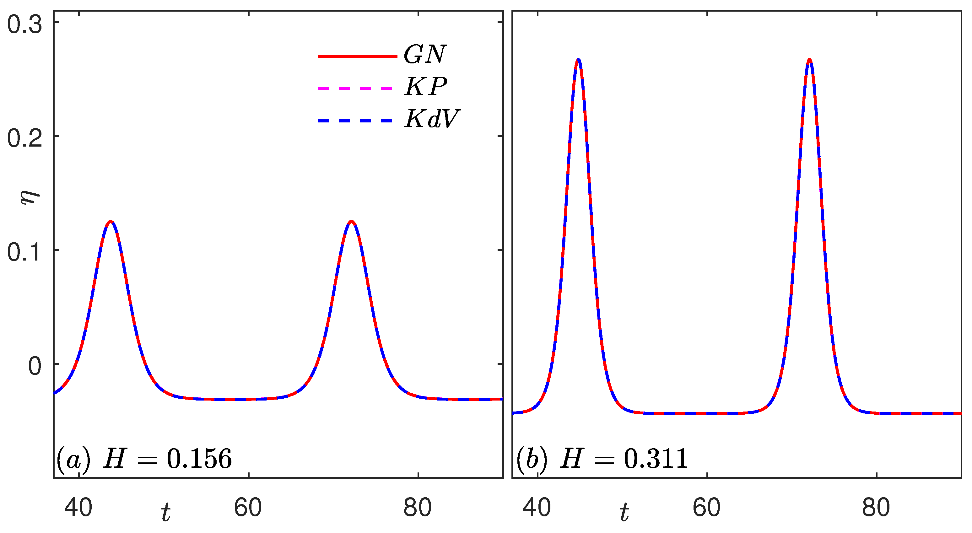
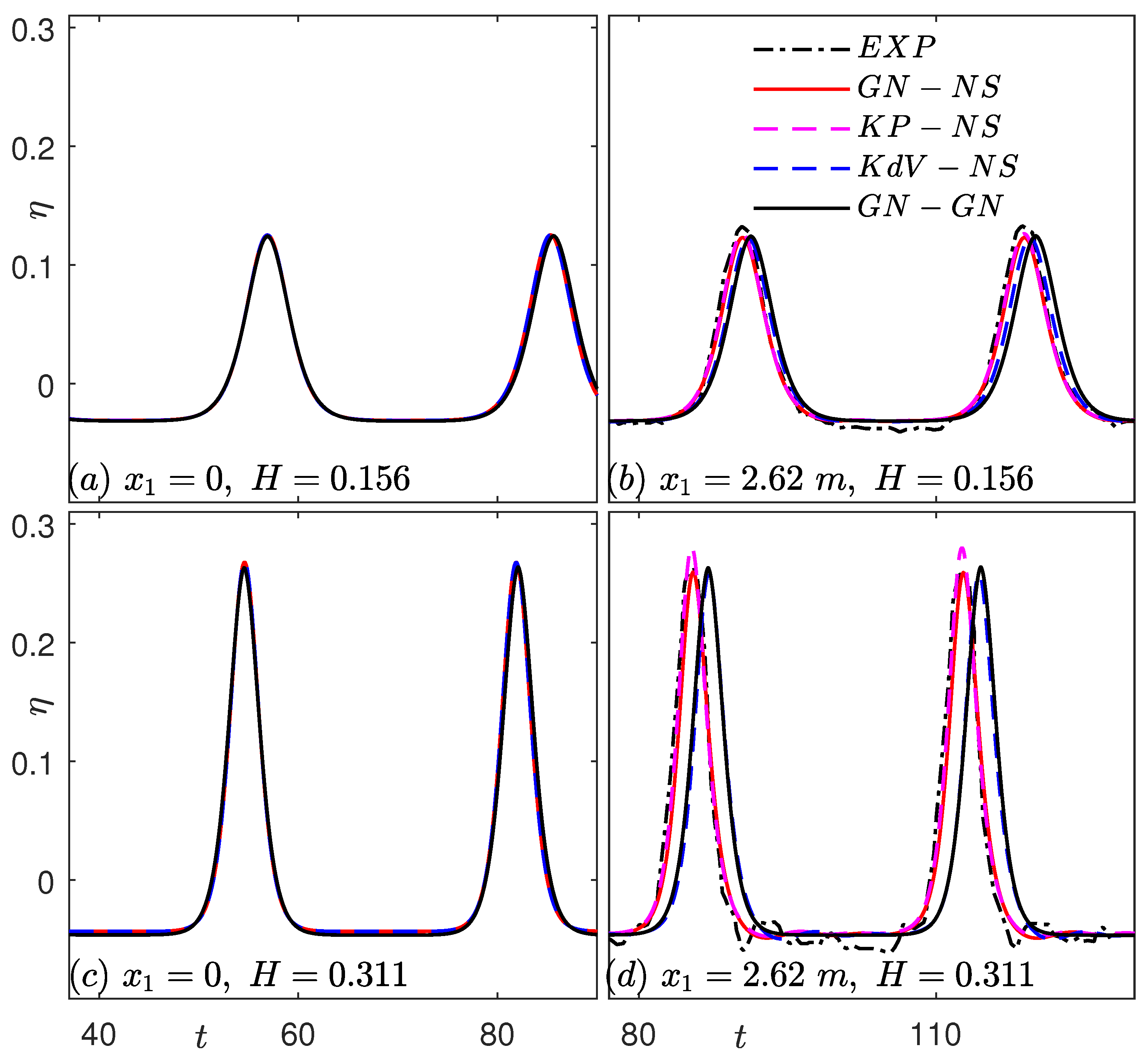
Figure 10.
Comparisons of surface elevation of cnoidal waves of GN-NS, KP-NS, KdV-NS and GN-GN and the laboratory measurements of [
43].
.
Figure 10.
Comparisons of surface elevation of cnoidal waves of GN-NS, KP-NS, KdV-NS and GN-GN and the laboratory measurements of [
43].
.
Figure 11.
Comparisons of pressure of cnoidal waves of various theories, propagating in domain of the NS and GN equations. .
Figure 11.
Comparisons of pressure of cnoidal waves of various theories, propagating in domain of the NS and GN equations. .
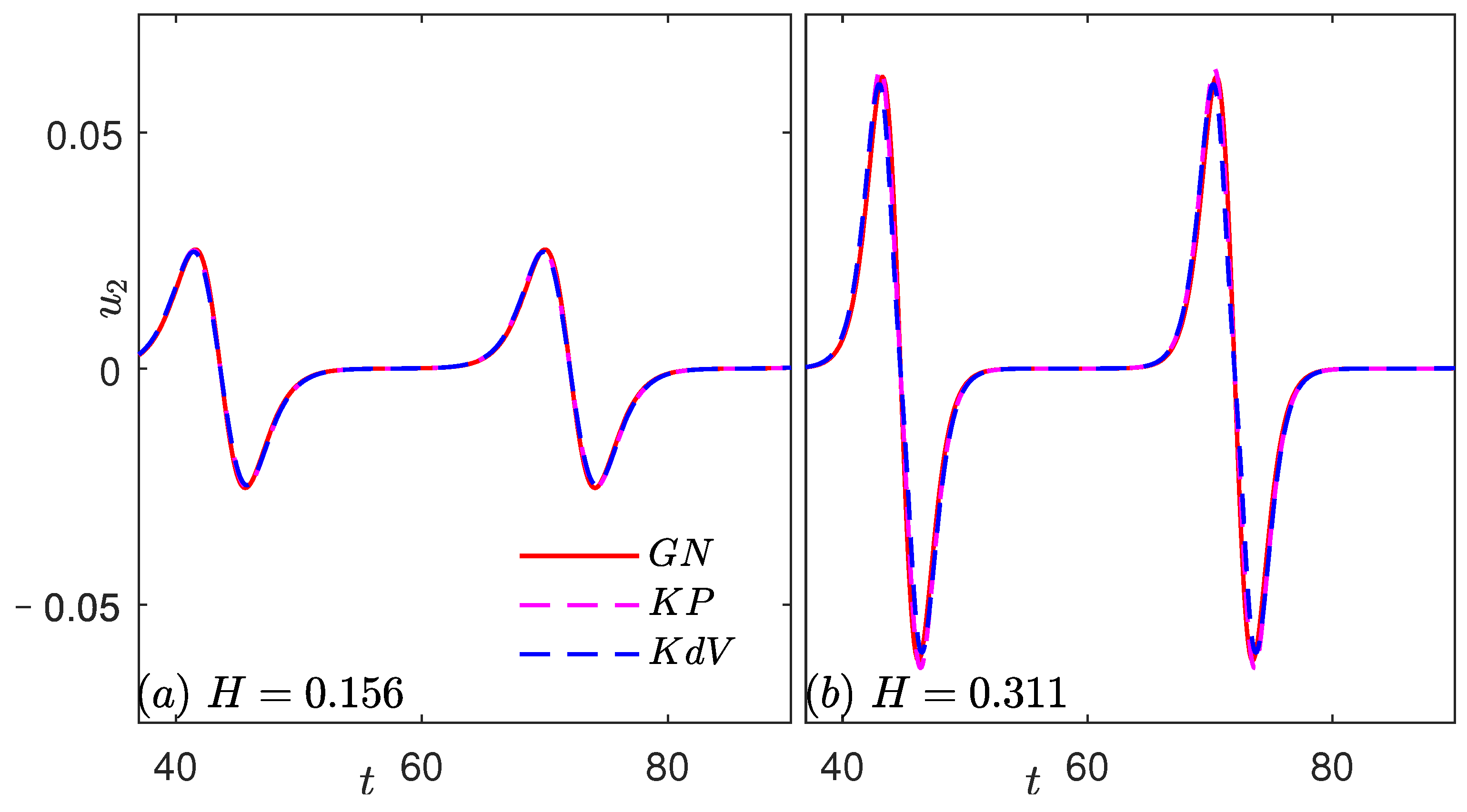
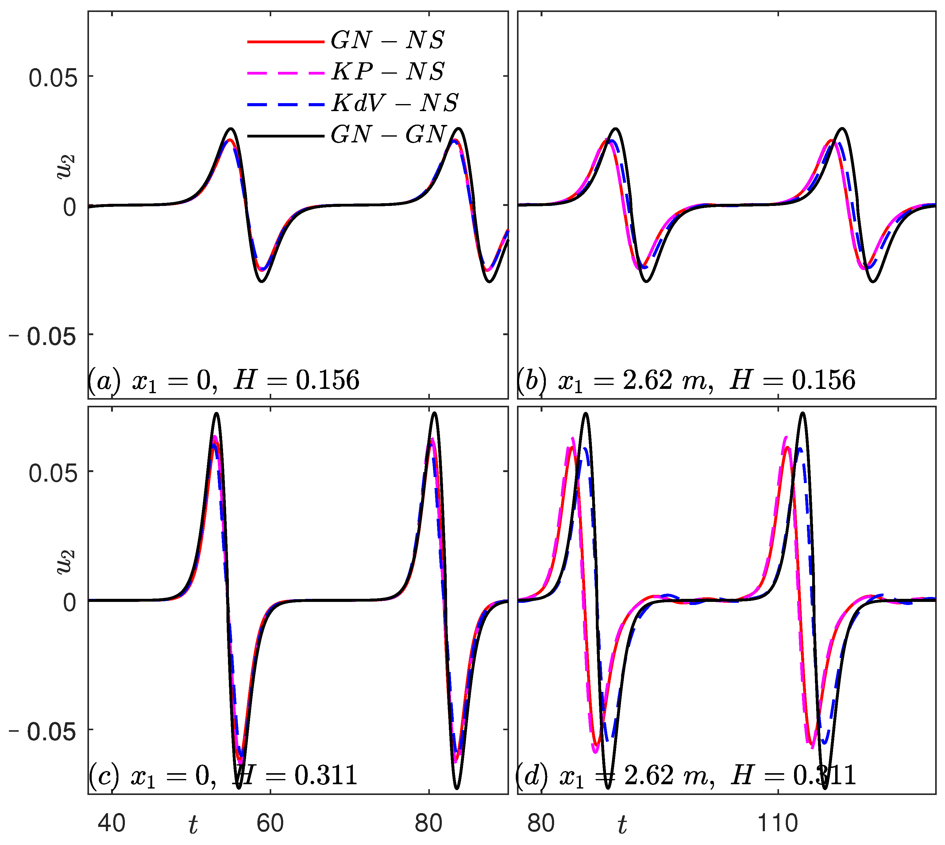
Figure 12.
Comparisons of horizontal particle velocity of cnoidal waves generated by various theories, propagating in domain of the NS equations. .
Figure 12.
Comparisons of horizontal particle velocity of cnoidal waves generated by various theories, propagating in domain of the NS equations. .
Figure 13.
Comparisons of vertical particle velocity of cnoidal waves generated by various theories, propagating in domain of the NS equations. .
Figure 13.
Comparisons of vertical particle velocity of cnoidal waves generated by various theories, propagating in domain of the NS equations. .
Figure 14.
Comparisons of horizontal velocity distribution of cnoidal waves of theories, propagating in domains of the NS and GN equations in Case 1. , .
Figure 14.
Comparisons of horizontal velocity distribution of cnoidal waves of theories, propagating in domains of the NS and GN equations in Case 1. , .
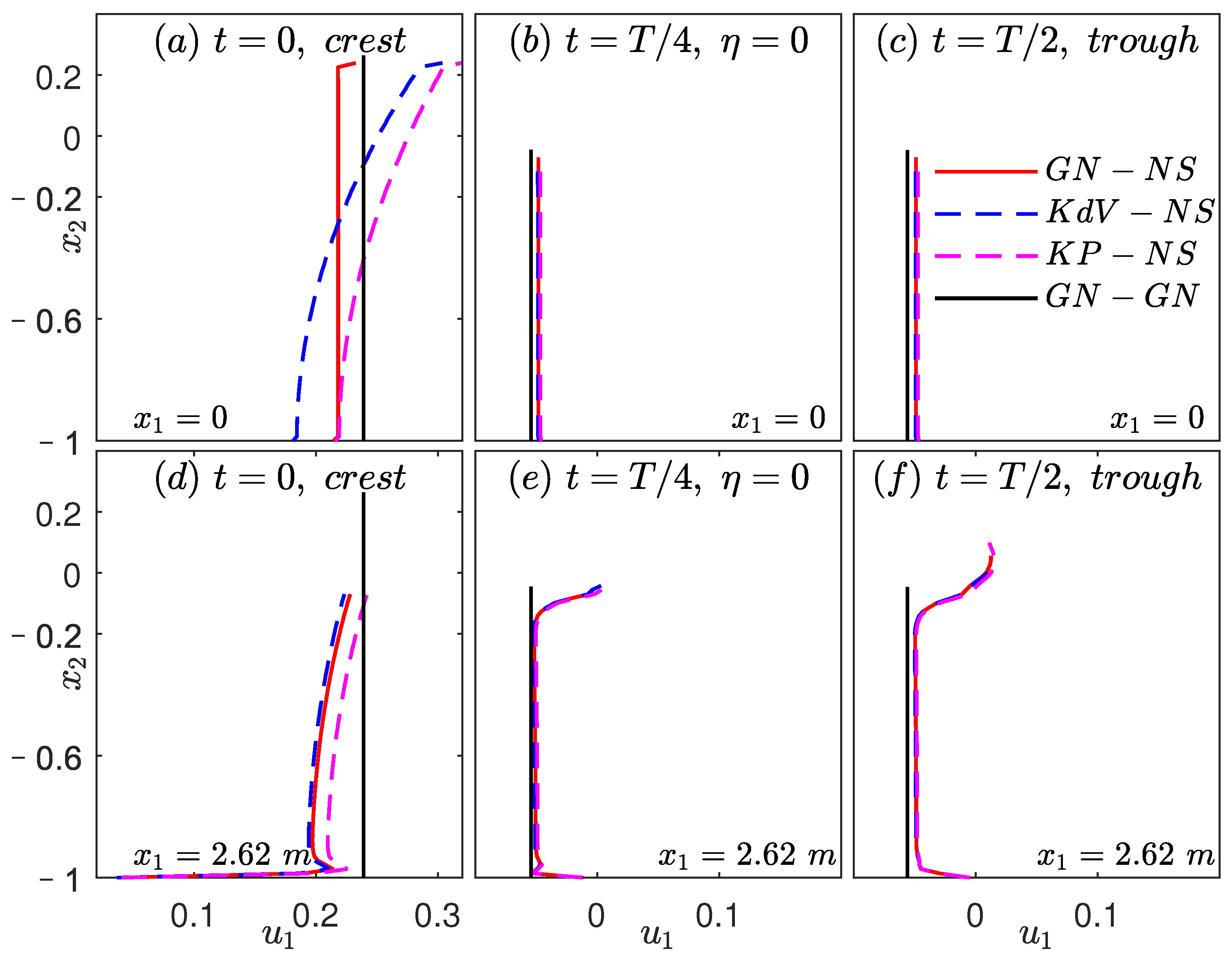
Figure 15.
Comparisons of horizontal velocity distribution of cnoidal waves of theories, propagating in domains of the NS and GN equations in Case 2. , .
Figure 15.
Comparisons of horizontal velocity distribution of cnoidal waves of theories, propagating in domains of the NS and GN equations in Case 2. , .
Figure 16.
Comparisons of vertical velocity distribution of cnoidal waves of theories, propagating in domains of the NS and GN equations in Case 1. , .
Figure 16.
Comparisons of vertical velocity distribution of cnoidal waves of theories, propagating in domains of the NS and GN equations in Case 1. , .
Figure 17.
Comparisons of vertical velocity distribution of cnoidal waves of theories, propagating in domains of the NS and GN equations in Case 2. , .
Figure 17.
Comparisons of vertical velocity distribution of cnoidal waves of theories, propagating in domains of the NS and GN equations in Case 2. , .
Table 1.
Solutions of solitary wave by different theories.
Table 1.
Solutions of solitary wave by different theories.
| | Boussinesq | KdV | Laitone’s 1st Order | Laitone’s 2nd Order | GN |
|---|
|
|
|
|
|
|
|
| C |
|
|
|
|
|
|
|
|
|
|
|
|
|
| |
|
|
|
|
Table 2.
Comparisons of the peak values of the surface elevation, horizontal and vertical velocities of cnoidal wave () of the GN equations and the KP equations.
Table 2.
Comparisons of the peak values of the surface elevation, horizontal and vertical velocities of cnoidal wave () of the GN equations and the KP equations.
| |
|
|
|
|---|
| GN | 0.1251 | 0.1145 | 0.0252 |
| KP | 0.1251 | 0.1219 | 0.0250 |
| R |
|
|
|
| KdV | 0.1251 | 0.1162 | 0.0247 |
| R |
|
|
|
Table 3.
Comparisons of the peak values of the surface elevation, horizontal and vertical velocities of cnoidal wave () of the GN equations and the KP equations.
Table 3.
Comparisons of the peak values of the surface elevation, horizontal and vertical velocities of cnoidal wave () of the GN equations and the KP equations.
| |
|
|
|
|---|
| GN | 0.2675 | 0.2273 | 0.0618 |
| KP | 0.2675 | 0.2580 | 0.0635 |
| R |
|
|
|
| KdV | 0.2674 | 0.2265 | 0.0603 |
| R |
|
|
|
Table 4.
List of the combination of wave makers and domain equations of the unsteady cases considered in this study.
Table 4.
List of the combination of wave makers and domain equations of the unsteady cases considered in this study.
| Case | Wave Maker Theory | Domain Governing Equations | Type of Waves |
|---|
| KdV-NS | KdV | NS | solitary & cnoidal |
| KP-NS | KP | NS | cnoidal |
| GN-NS | GN | NS | solitary & cnoidal |
| GN-GN | GN | GN | solitary & cnoidal |
Table 5.
Solitary wave cases considered in this study.
Table 5.
Solitary wave cases considered in this study.
| Case | A |
|---|
| 1 | 0.192 |
| 2 | 0.301 |
| 3 | 0.408 |
| 4 | 0.525 |
Table 6.
The analytical and numerical wave speeds of various theories ().
Table 6.
The analytical and numerical wave speeds of various theories ().
| | | Analytical | Value of C |
|---|
| Steady-state | Boussinesq Theory |
| 1.1832 |
| Laitone’s 1st Theory |
| 1.2000 |
| Laitone’s 2st Theory |
| 1.1760 |
| GN Theory |
| 1.1832 |
| KdV equations |
| 1.1832 |
| Unsteady | KdV-NS | | 1.1767 |
| GN-NS | | 1.1769 |
| GN-GN | | 1.1769 |
Table 7.
Cnoidal wave cases considered in this study.
Table 7.
Cnoidal wave cases considered in this study.
| Case |
| H |
|---|
| 1 | 29.6 | 0.156 |
| 2 | 29.6 | 0.311 |
Table 8.
The percentage differences between the peak of the surface elevation of cnoidal waves of different models and the laboratory measurements of [
43].
.
Table 8.
The percentage differences between the peak of the surface elevation of cnoidal waves of different models and the laboratory measurements of [
43].
.
| Case |
|
|
|---|
| Experiments | 0.132 | 0.262 |
| GN-NS | 0.123 | 0.259 |
| R |
|
|
| KP-NS | 0.126 | 0.280 |
| R |
|
|
| KdV-NS | 0.123 | 0.257 |
| R |
|
|
| GN-GN | 0.125 | 0.264 |
| R |
|
|
Table 9.
The differences between the peak pressure of cnoidal waves generated by various theories.
Table 9.
The differences between the peak pressure of cnoidal waves generated by various theories.
| Case |
|
|
|---|
| GN-GN | 1.124 | 1.263 |
| GN-NS | 1.100 | 1.201 |
| R |
|
|
| KP-NS | 1.108 | 1.216 |
| R |
|
|
| KdV-NS | 1.105 | 1.200 |
| R |
|
|
Table 10.
The differences between the peak horizontal velocity of cnoidal waves generated by various theories.
Table 10.
The differences between the peak horizontal velocity of cnoidal waves generated by various theories.
| Case |
|
|
|---|
| GN-GN | 0.121 | 0.242 |
| GN-NS | 0.114 | 0.220 |
| R |
|
|
| KP-NS | 0.117 | 0.235 |
| R |
|
|
| KdV-NS | 0.114 | 0.219 |
| R |
|
|
Table 11.
The differences between the peak vertical velocity of cnoidal waves generated by various theories.
Table 11.
The differences between the peak vertical velocity of cnoidal waves generated by various theories.
| Case |
|
|
|---|
| GN-GN | 0.0296 | 0.0726 |
| GN-NS | 0.0250 | 0.0592 |
| R |
|
|
| KP-NS | 0.0255 | 0.0632 |
| R |
|
|
| KdV-NS | 0.0249 | 0.0588 |
| R |
|
|


