Model Predictive Controller Design Based on Residual Model Trained by Gaussian Process for Robots

Abstract

Model mismatch is inevitable in robot control due to the presence of unknown dynamics and unknown perturbations. Traditional model predictive control algorithms are usually based on constant value assumptions and are not able to overcome the degradation of controller performance due to model mismatch. In this paper, a model predictive control (MPC) algorithm based on Gaussian process regression (GPR) is proposed. Firstly, the kinematic equations of the mobile robot are established by the mechanistic analysis method; similarly, the dynamics of the mobile robot system are modeled using the second-class Lagrangian equations. Secondly, the problem of stability and reliability degradation due to model mismatch during the operation of mobile robot is considered. This paper uses a MPC algorithm with a main model plus residual model to solve the MPC closed-loop control strategy. The state at each moment is decomposed into a predicted state based on the first-principles model and a residual state. The residual state is learned by GPR in real-time and used to compensate for deviations between the real process model and the predicted model. The proposed method requires fewer data samples, enhancing the technique’s practicality. Finally, the simulation results show that the proposed algorithm is more stable and achieves the desired tracking faster. Compared with the MPC algorithm, the arrival time of the system is reduced by 28% and the speed error is controlled within 0.07.

1. Introduction

Omnidirectional mobile robots have good stability and load-bearing capacity [1,2]. Mobile robots have great application potential in high-end manufacturing fields such as aviation, aerospace, and industrial transportation [3]. However, their complex gear train structure renders them difficult to accurately control. In [4], the dynamic equation of a mobile robot was proposed, which was derived using the second Lagrange equation. In [5], a two-stage control system was designed to realize the indoor navigation of the robot. It is well known that the dynamic model of a mobile robot is highly nonlinear and contains model uncertainties. In addition, it is necessary to consider the input saturation constraint, which brings significant challenges to dynamic control [6].

Trajectory tracking control is one of the main problems of mobile robots control. Accurate trajectory tracking is also the first prerequisite for mobile robots to complete their tasks. In the previous research on trajectory tracking, the control is based on the precise attitude information of the mobile robots, and it is assumed that the ideal speed tracking of the mobile robots can be dynamically realized [7]. However, this situation is too idealistic. In practical applications, it is difficult to achieve ideal speed tracking due to the influence of errors and disturbances. Aiming at such problems, the literature [8] proposed a nonlinear disturbance observer technique to estimate disturbance and compensate for modelling errors. Considering the unknown disturbance and uncertainty, a sliding mode control method based on extended state observer is proposed for the trajectory tracking of mobile robots [9]. In addition, a fuzzy-model-based control framework deals with vehicle dynamics and highly uncertain behavior [10].

MPC is widely used in trajectory tracking control of mobile robots due to its robustness and stability [11]. This is because MPC provides a method that incorporates both goals and constraints. However, in the practical application of MPC, model mismatch is inevitable. It comes from modeling errors caused by external disturbances and system modeling errors. This also means that MPC needs to fully consider the model’s uncertainty and adaptively update the model. Luo et al. [12] designed a heterogeneous robust MPC with modelling uncertainty and external disturbances. Cao et al. [13] further control the tracking error through constraint transformation in MPC to reduce the workload of tracking error control. In [14], an MPC planning controller is proposed to enable path planning systems for autonomous vehicles to cleanly handle different obstacles and road structures while exploiting vehicle dynamics for optimal path planning. In [15], Rasekhipour et al. provided a vehicle collision avoidance path planning and tracking method based on multi-constraint model predictive control. They used the Hildreth quadratic programming method to solve it. In [16], Ji designed a high-speed obstacle avoidance path planning algorithm based on real-time output constraints MPC. In [17], Kim et al. proposed an MPC-based trajectory tracking implementation that considers the road’s feasible area and the vehicle’s shape. In [18], Guo et al. proposed a quasi-infinite time-domain nonlinear MPC scheme for general reference trajectory tracking, which obtains available terminal-reachable trajectories without increasing online computational complexity.

1.1. Related Work

With the rapid development of machine learning in recent years, many “learning” ideas have also been introduced into model predictive control [19,20]. Aswani [21] was the first to propose learning-based model predictive control (LBMPC), which has been the subject of intensive research for more than ten years. In recent reports, many LBMPC algorithms have emerged [22,23,24].

The LBMPC algorithm aims to mine historical and/or online operating data, using machine learning algorithms to improve the accuracy of the predictive model or optimize the controller design, thereby improving the control quality of the closed-loop system. The LBMPC algorithm considers using data collected online (such as input and output or state measurements) to update the model and/or describe the uncertainty. Recently, the LBMPC control strategy has been widely used in mobile robot control.

The combination of robust reachability guarantees of control theory with Bayesian analysis based on empirical observations guarantees that the constraints of MPC are satisfied. In [25], Zhang et al. propose an adaptive LBMPC scheme for track tracking of disturbed ground vehicles subject to input constraints.

Due to the existence of model uncertainty, algorithms such as learning system models are similar to adaptive MPC algorithms. The work mainly focuses on using some machine learning algorithms (such as neural networks [25,26], reinforcement learning [27], etc.) to learn MPC offline or online. The controller’s internal model or uncertainty description and the MPC controller’s design are based on the learned model. To realize the real-time response of the controller, the literature [24,28,29] uses a deep neural network to train the sample database offline. However, such methods rely too much on prior knowledge [30]. The literature results [31] show that GPR requires less prior process knowledge, can directly provide a measure of the uncertainty of the residual model, and improve control performance by learning periodic time-varying disturbances. As a supervised learning method, GPR improves robustness to overfitting under small data conditions by applying a “kernel trick” to implicitly compute in a high-dimensional space since there is no need to check an uncountable set of possible functions when using the training data for regression. In a recent report, the literature [32,33] utilizes the uncertainty variation in the GP learning process to ensure the system’s stability.

Lukas et al. [34] propose using GP as a prediction function to model the residuals and test the proposed method in a racing path planning scenario. The results show that the performance and security of the controller can be improved significantly.

Bonzanini et al. [35] proposed a GPs-based strategy to monitor model changes due to model-plant mismatch.

1.2. Contributions

Although model uncertainty and unknown disturbances are considered in the existing studies, few studies on the mobile robots have considered these factors simultaneously. Ignoring these factors in robot control may reduce the stability of the system. Based on the above analysis and considering the problem of degraded MPC closed-loop control performance, we aim to train a residual model using GPR to learn the deviation of the main model from the mobile robot dynamics to complement the prediction results further.

We use a GPR-MPC control strategy with a main model plus a residual model. Where the main model is used to describe the main dynamic relationship between the input and the state. The residual model is trained with GPR. The state and input-dependent uncertainty model describes the relationship between the state of the controlled object and the actual state using GPR to correct the estimation results. In the initial moment, the state of the controlled object is used as the initial main model state. Then the main model’s and residual model’s output are predicted based on the control inputs to be optimized. The sum of the two is the estimate of the actual state. In the second prediction step, the main model state is used as the base point to predict the main model’s output and the residual model’s output corresponding to the inputs to be optimized, respectively. In this way, it is iterated until the end of the prediction time domain. The method proposed in this paper updates the mismatch model of the prediction error of the MPC controller for the control action online. It improves the performance of the MPC controller.

2. Mobile Robot Kinematics Model

The kinematic model of a mobile robot is modeled by analyzing its motion law and using the mechanism analysis method because its actuator spacing, geometric center and other parameters are known or measurable, and the kinematic model is relatively simple.

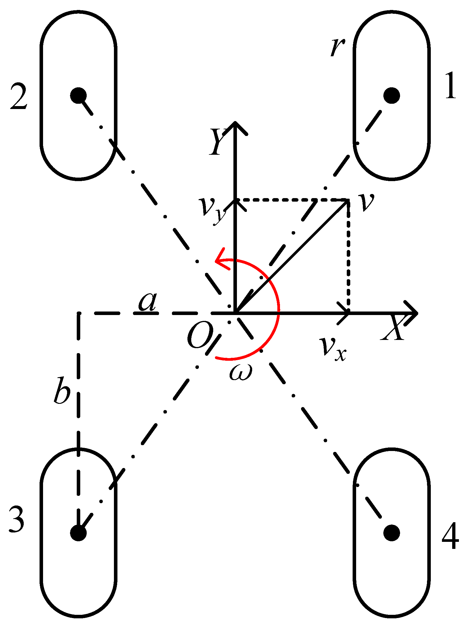
The mobile robots mechanism is mounted on the chassis in an O-rectangular layout. Assume that the mobile robot actuator is a rigid body. Firstly, the coordinate system $xoyz$ of the mobile robot itself is established, and the geometric center of the mobile robot is its coordinate origin O. The motion of the mobile robot is decomposed into three separate parts, which are as follows: the translation in the x-axis direction, the translation in the y-axis direction and the rotation around the z-axis (vertical xoy plane outward). The body is specified as the positive direction of the x-axis in the right direction, the positive direction of the y-axis in the forward direction and the counterclockwise direction is the positive direction of rotation around the z-axis. Schematic diagram of mobile robot mechanism is shown in Figure 1.

The meaning of the parameters are listed below,

• O denotes the geometric center of the mobile robot.
• $\overrightarrow{v}$ denotes the translational velocity of the mobile robot in its own coordinate system.
• ${\overrightarrow{v}}_x$ denotes the component of the mobile robot in the x-axis direction in its own coordinate system.
• ${\overrightarrow{v}}_y$ denotes the component of the mobile robot in the direction of y-axis in its own coordinate system.
• $\overrightarrow{\omega }$ denotes the rotation speed of the mobile robot around its geometric center in its own coordinate system.
• a denotes the distance from the center of the mobile robot axis in the x-axis direction to the geometric center of the mobile robot mechanism.
• b denotes the distance from the axis center of the mobile robot in the y-axis direction to the geometric center of the mobile robot mechanism.
• r denotes the radius of the mobile robot.

Specify ${\overrightarrow{v}}_1$, ${\overrightarrow{v}}_2$, ${\overrightarrow{v}}_3$, and ${\overrightarrow{v}}_4$ as the axial velocities of actuator 1, actuator 2, actuator 3 and actuator 4, respectively; ${\overrightarrow{\omega }}_1$, ${\overrightarrow{\omega }}_2$, ${\overrightarrow{\omega }}_3$, and ${\overrightarrow{\omega }}_4$ as the angular velocities of actuator 1, actuator 2, actuator 3 and actuator 4, respectively, and the counterclockwise rotation direction is positive.

As the mobile robot moves in the direction of the x-axis.

$$\left\{\begin{array}{c}{\overrightarrow{v}}_1=-{\overrightarrow{v}}_x\\ {\overrightarrow{v}}_2=+{\overrightarrow{v}}_x\\ {\overrightarrow{v}}_3=-{\overrightarrow{v}}_x\\ {\overrightarrow{v}}_4=+{\overrightarrow{v}}_x\end{array}\right.$$

(1)

As the mobile robot moves in the direction of the y-axis.

$$\left\{\begin{array}{c}{\overrightarrow{v}}_1={\overrightarrow{v}}_y\\ {\overrightarrow{v}}_1={\overrightarrow{v}}_y\\ {\overrightarrow{v}}_1={\overrightarrow{v}}_y\\ {\overrightarrow{v}}_1={\overrightarrow{v}}_y\end{array}\right.$$

(2)

As the mobile robot rotates around its geometric center.

$$\left\{\begin{array}{c}{\overrightarrow{v}}_1=+\overrightarrow{\omega }\left(a+b\right)\\ {\overrightarrow{v}}_2=+\overrightarrow{\omega }\left(a+b\right)\\ {\overrightarrow{v}}_3=+\overrightarrow{\omega }\left(a+b\right)\\ {\overrightarrow{v}}_4=+\overrightarrow{\omega }\left(a+b\right)\end{array}\right.$$

(3)

The general speed relationship for the motion of the driven mechanism in the plane can be obtained by summing the three aforementioned motions as follows

$$\left\{\begin{array}{c}{\overrightarrow{v}}_1=-{\overrightarrow{v}}_x+{\overrightarrow{v}}_y+\overrightarrow{\omega }\left(a+b\right)\\ {\overrightarrow{v}}_2=+{\overrightarrow{v}}_x+{\overrightarrow{v}}_y-\overrightarrow{\omega }\left(a+b\right)\\ {\overrightarrow{v}}_3=-{\overrightarrow{v}}_x+{\overrightarrow{v}}_y-\overrightarrow{\omega }\left(a+b\right)\\ {\overrightarrow{v}}_4=+{\overrightarrow{v}}_x+{\overrightarrow{v}}_y+\overrightarrow{\omega }\left(a+b\right).\end{array}\right.$$

(4)

The collation leads to

$$\left[\begin{array}{c}{\overrightarrow{v}}_1\\ {\overrightarrow{v}}_2\\ {\overrightarrow{v}}_3\\ {\overrightarrow{v}}_4\end{array}\right]=\left[\begin{array}{ccc}\begin{array}{c}-1\\ 1\\ -1\\ 1\end{array}& \begin{array}{c}1\\ 1\\ 1\\ 1\end{array}& \begin{array}{c}a+b\\ -\left(a+b\right)\\ -\left(a+b\right)\\ a+b\end{array}\end{array}\right]\left[\begin{array}{c}{\overrightarrow{v}}_x\\ {\overrightarrow{v}}_y\\ \overrightarrow{\omega }\end{array}\right].$$

(5)

Let

$$J\left(\alpha \right)=\left[\begin{array}{ccc}\begin{array}{c}-1\\ 1\\ -1\\ 1\end{array}& \begin{array}{c}1\\ 1\\ 1\\ 1\end{array}& \begin{array}{c}a+b\\ -\left(a+b\right)\\ -\left(a+b\right)\\ a+b\end{array}\end{array}\right],$$

that is:

$$\left[\begin{array}{c}{\overrightarrow{v}}_1\\ {\overrightarrow{v}}_2\\ {\overrightarrow{v}}_3\\ {\overrightarrow{v}}_4\end{array}\right]=J\left(\alpha \right)\left[\begin{array}{c}{\overrightarrow{v}}_x\\ {\overrightarrow{v}}_y\\ \overrightarrow{\omega }\end{array}\right].$$

(6)

The above Equation (6) is the inverse kinematic equation of the mobile robot. The matrix $J\left(\alpha \right)$ represents the mapping relationship from ${\left[{\overrightarrow{v}}_x,{\overrightarrow{v}}_y,\overrightarrow{\omega }\right]}^T$ to ${\left[\begin{array}{c}{\overrightarrow{v}}_1,{\overrightarrow{v}}_2,{\overrightarrow{v}}_3,{\overrightarrow{v}}_4\end{array}\right]}^T$. According to Equation (6), it is known that the velocity of each actuator can be solved by the velocity components of the whole mechanism in each direction.

The inverse kinematic equation of the omnidirectional mobile robot mechanism embodies the velocity of the omnidirectional mobile robot as a function of the velocity of each actuator. The kinematic properties of the drive mechanism can be represented by the Jacobi matrix of the inverse kinematic equations. When the Jacobi matrix of inverse kinematics is not full rank, the omnidirectional mobile robot will have singularities during motion, i.e., the robot loses degrees of freedom during motion and does not have omnidirectional motion capability. Therefore, the Jacobi matrix of the inverse kinematic equations is a full rank matrix, which is necessary for the robot to have omnidirectional mobility.

The generalized inverse kinematic equation $J{\left(\alpha \right)}^{+}$ can be obtained by performing a matrix transformation on J.

$$J{\left(\alpha \right)}^{+}={\left(J{\left(\alpha \right)}^{T}J\left(\alpha \right)\right)}^{-1}J{\left(\alpha \right)}^T=\frac{1}{4}\left[\begin{array}{cccc}\begin{array}{c}-1\\ 1\\ \frac{1}{a+b}\end{array}& \begin{array}{c}1\\ 1\\ -\frac{1}{a+b}\end{array}& \begin{array}{c}-1\\ 1\\ -\frac{1}{a+b}\end{array}& \begin{array}{c}1\\ 1\\ \frac{1}{a+b}\end{array}\end{array}\right]$$

(7)

Therefore, the kinematic equations of the mobile robot during horizontal travel are as follows.

$$\left[\begin{array}{c}{\overrightarrow{v}}_x\\ {\overrightarrow{v}}_y\\ \overrightarrow{\omega }\end{array}\right]=\frac{1}{4}\left[\begin{array}{cccc}\begin{array}{c}-1\\ 1\\ \frac{1}{a+b}\end{array}& \begin{array}{c}1\\ 1\\ -\frac{1}{a+b}\end{array}& \begin{array}{c}-1\\ 1\\ -\frac{1}{a+b}\end{array}& \begin{array}{c}1\\ 1\\ \frac{1}{a+b}\end{array}\end{array}\right]\left[\begin{array}{c}{\overrightarrow{v}}_1\\ {\overrightarrow{v}}_2\\ {\overrightarrow{v}}_3\\ {\overrightarrow{v}}_4\end{array}\right]$$

(8)

Converting the axial velocity of an actuator to its angular velocity can be achieved with the following equation.

$$\left[\begin{array}{c}{\overrightarrow{v}}_x\\ {\overrightarrow{v}}_y\\ \overrightarrow{\omega }\end{array}\right]=\frac{r}{4}\left[\begin{array}{cccc}\begin{array}{c}-1\\ 1\\ \frac{1}{a+b}\end{array}& \begin{array}{c}1\\ 1\\ -\frac{1}{a+b}\end{array}& \begin{array}{c}-1\\ 1\\ -\frac{1}{a+b}\end{array}& \begin{array}{c}1\\ 1\\ \frac{1}{a+b}\end{array}\end{array}\right]\left[\begin{array}{c}{\omega }_1\\ {\omega }_2\\ {\omega }_3\\ {\omega }_4\end{array}\right]$$

(9)

3. Mobile Robot Dynamics Model

As with the kinematic model, the kinetic modeling is performed by analyzing its kinematic laws using the mechanism analysis method because its specific parameters can be measured or easily estimated, and the model is relatively simple.

The dynamics is modeled using the Lagrangian method. In order to simplify the model and facilitate the analysis, the following assumptions were made.

Assumption A1.

The potential energy of a mobile robot traveling on a horizontal surface remains constant at 0.

Assumption A2.

The inertia of the mobile robot is neglected.

Assumption A3.

The robot’s own coordinate system is located on its center of gravity.

The kinetic energy of the system $E_k$

$$E_k=\frac{1}{2}m(v_x^2+v_y^2)+\frac{1}{2}{I}_Z{\omega }^2+\frac{1}{2}{I}_{\omega }{\sum }_{i=1}^4{\omega }_i^2$$

(10)

According to the kinematic equation established by Equation (8), the following equation is obtained:

$$\left\{\begin{array}{c}{v}_X^2={\left(\frac{r}{4}\times \left(-{\omega }_1+{\omega }_2-{\omega }_3+{\omega }_4\right)\right)}^2\\ v_Y^2={\left(\frac{r}{4}\times \left({\omega }_1+{\omega }_2+{\omega }_3+{\omega }_4\right)\right)}^2\\ {\omega }^2={\left(\frac{r}{4}\times \frac{1}{a+b}\times \left({\omega }_1-{\omega }_2-{\omega }_3+{\omega }_4\right)\right)}^2\end{array}\right.$$

(11)

where m is the total mass of the mobile robot; $I_Z$ is the rotational inertia of the mobile robot in the z-axis direction; $I_{\omega }$ is the rotational inertia of the actuator; and ${\omega }_i$ is the angular velocity of the i-th ($i=1,2,3,4$) actuator.

From the second type of Lagrangian equation, we get

$$\frac{d}{dt}\left(\frac{\partial L}{\partial \dot{q}}\right)-\frac{\partial L}{\partial q}=\tau$$

(12)

where q denotes the generalized coordinates, which in this paper are expressed as the coordinates and the positional offset angle of the mobile robot in the world coordinate system; $\dot{q}$ denotes the generalized velocity, which is the differentiation of the generalized coordinates; and L denotes the Lagrangian function, which is equal to the kinetic energy of the system minus the potential energy of the system. The potential energy of the system is 0; so, the Lagrangian function of mobile robot system is its kinetic energy. $\tau$ denotes the generalized force, which in this thesis represents the inertial driving moment of the actuator.

Considering the effect of friction in the internal structure of the mobile robot. Force analysis for each actuator can be obtained:

$$T=\tau +T_g+T_f$$

(13)

where T denotes the total driving moment to which the actuator is subjected. $T_g$ denotes the frictional moment of actuator. $T_f$ denotes the frictional moment applied to the axle center when the actuator is rotating.

The friction moment $T_g$ is also the load moment of the robot, which is related to the mass m of the robot and the coefficient of friction $\mu$ of actuator, and the weight of the robot is divided equally among the four actuators. The following equation is shown.

$$T_g=\mu \frac{mg}{4}r$$

(14)

The friction torque $T_f$ is related to the speed ${\omega }_i$ of the actuator and the axial viscous friction coefficient f of the actuator, as shown in the following equation.

$$T_f=f{\omega }_i$$

(15)

Since the ratio between the actuators and the motor in the mobile robot system is 1, the driving torque and the electromagnetic torque of the machine are equal and can be obtained as follows.

$$T=T_g$$

(16)

According to the electromagnetic torque equation of the brushless DC motor, $T_e=\frac{p·2e_a{i}_a}{\omega }=p·K_{T}i$, and joint Equations (13) and (16), we can get

$$p·K_{T}i=\tau +\mu \frac{mg}{4}r+f\omega .$$

(17)

Considering the mobile robot system from a single actuator, the association of Equations (11), (12) and (17) yields

$$p{K}_T\left[\begin{array}{c}{i}_1\\ i_2\\ i_3\\ i_4\end{array}\right]=M\left[\begin{array}{c}{\omega }_1\\ {\omega }_2\\ {\omega }_3\\ {\omega }_4\end{array}\right]+f\left[\begin{array}{c}{\omega }_1\\ {\omega }_2\\ {\omega }_3\\ {\omega }_4\end{array}\right]+\mu \frac{mg}{4}r\left[\begin{array}{c}1\\ 1\\ 1\\ 1\end{array}\right].$$

(18)

where

$$M=\left[\begin{array}{cccc}\begin{array}{c}C\\ -B\\ D\\ B\end{array}& \begin{array}{c}-B\\ C\\ B\\ D\end{array}& \begin{array}{c}D\\ B\\ C\\ -B\end{array}& \begin{array}{c}B\\ D\\ -B\\ C\end{array}\end{array}\right],$$

(19)

$$\left\{\begin{array}{c}A=\frac{m{r}^2}{8}\\ B=\frac{I_Z{r}^2}{16{\left(a+b\right)}^2}\\ C=A+B+I_{\omega }\\ D=A-B\end{array}\right.$$

(20)

The collation of Equation (18) leads to a drive dynamics model for a mobile robot containing a DC brushless motor model.

$$\left[\begin{array}{c}{i}_1\\ i_2\\ i_3\\ i_4\end{array}\right]=\frac{M}{p{K}_T}\left[\begin{array}{c}{\omega }_1\\ {\omega }_2\\ {\omega }_3\\ {\omega }_4\end{array}\right]+\frac{f}{p{K}_T}\left[\begin{array}{c}{\omega }_1\\ {\omega }_2\\ {\omega }_3\\ {\omega }_4\end{array}\right]+\mu \frac{mg}{4p{K}_T}r\left[\begin{array}{c}1\\ 1\\ 1\\ 1\end{array}\right]$$

(21)

where $\left[\begin{array}{c}{i}_1,i_2,i_3,i_4\end{array}\right]$ denotes the input matrix of the control current of the system.

4. Gaussian Process Based Model Predictive Control

According to the kinematic model of the mobile robot traveling on the plane, it is known that the mobile robot can achieve the omnidirectional motion of any attitude in three degrees of freedom in the plane. The controller designed in this section expects that the mobile robot can move according to the desired trajectory with low error state as much as possible under the control and regulation of the controller, and reach the desired location to improve the stability and reliability of the robot at work. In this section, the kinematic model of the mobile robots, the driving method, and the GPR-based model predictive control algorithm are used to design the controller to study the relationship between the speed and position of the mobile robots.

4.1. Model Predictive Control

The form of the optimization problem to be solved by the GPR-MPC algorithm is given in this section. As shown in Figure 2, the Mpc control strategy block diagram is mainly composed of an optimizer and a GPR-based master and residual model. We consider a general nonlinear dynamical system that can be modeled as

$$x_{k+1}=f\left(x_k,u_k\right)$$

(22)

where $x\in {\mathbb{R}}^{n_x}$ denotes the state vector and $u\in {\mathbb{R}}^{n_u}$ denotes the input vector. It is assumed that both the state and the input vary in a bounded range and that the controlled system has no measurement noise in order to avoid the interference of measurement noise affecting the effectiveness of GPR model modeling. In the above equation, $f(·)$ represents the modelable relation, which is the modelable part of the controlled system and is assumed to be linear.

Next, some necessary assumptions utilized in the following sections are given below. These assumptions ensure the existence and uniqueness of the solution of the MPC initial value problem.

Assumption A4.

The nonlinear System (27) is controllable and observable. $f:\mathcal{X}\times \mathcal{U}\to \mathcal{X}$ is a continuous Lipschitz function.

Assumption A5.

For the initial conditions, the System (27) has a unique solution, that is, there exists an optimal control policye ${\pi }^{*}$.

The use of state feedback can improve the closed-loop dynamics of the system, especially when the controlled object itself does not have stability. Here, closed-loop feedback is added to the main model to form a control law:

$$u_k=-K{x}_k^f.$$

(23)

To differentiate the representation, the main state of the model is denoted as $x^f$ and the state of the residual model is represented as $x^g$. The feedback gain K can be designed according to the system requirements.

To differentiate the representation, ${\widehat{x}}_k$ is used to denote the estimation of the actual state vector, and the prediction model is the sum of the main model and the residual model.

$${\widehat{x}}_k=x_k^f+x_k^g$$

(24)

At the initial moment, the state $x_k$ of the controlled object is used as the initial main model state, and then the output $x_{k+1}^f$ of the main model and the output $x_{k+1}^g$ of the residual model are predicted based on the control input $u_k$ to be optimized, and the sum of the two is an estimate of the actual state ${\widehat{x}}_{k+1}$.

In the actual system, due to some physical constraints of the equipment itself or the need to meet some security constraints in the operation process, it is usually required that the input and output of the system and some intermediate variables meet specific constraints. The system state and input are constrained by

$$\begin{array}{c}x\left(k\right)\in \mathcal{X}=\left\{x\left(k\right)\left|-x_{min}\le x\left(k\right)\le x_{max}\right.\right\}\subseteq {\mathbb{R}}^n,\hfill \\ u\left(k\right)\in \mathcal{U}=\left\{u\left(k\right)\left|-u_{min}\le u\left(k\right)\le u_{max}\right.\right\}\subseteq {\mathbb{R}}^m,\hfill \end{array}$$

(25)

where each element of $x_{min}$, $x_{max}$, $u_{min}$ and $u_{max}$ is positive real number.

The performance index function should ensure that the mobile robot can track the reference trajectory quickly and smoothly. After consulting the references and considering the use of many performance index functions in the trajectory tracking of the mobile robot, the following performance index functions will be used:

$$\begin{array}{c}\underset{\Pi }{min}\begin{array}{cc}& J(x,\Pi )={∥x\left(N\right)∥}_F^2+{\displaystyle \sum _{k=0}^{N-1}}{∥x\left(k\left|k\right.\right)∥}_Q^2+{∥u\left(k\left|k\right.\right)∥}_R^2\end{array}\hfill \\ s.t.\begin{array}{cc}& \begin{array}{c}x(k+1\left|k\right.)=f(x\left(k\right),u\left(k\right))\hfill \\ u\left(k\right)=\pi \left(x\right(k\left)\right)\hfill \\ x\left(k\right)\in X\hfill \\ u\left(k\right)\in U\hfill \end{array}\end{array}\hfill \end{array}$$

(26)

where $Q>0$,$R>0$ and $F>0$ are symmetric weighting matrices; $x(k+i\left|k\right.)$ refers to the predicted value of the measured state vector at time $k+i$ based on the measured value at time k, and $x\left(k\left|k\right.\right)$ represents the measured value of the measured state vector at time k.$u(k+i\left|k\right.)$ represents the control input at time $k+i$ calculated by the optimization problem at time k, and $u\left(k\left|k\right.\right)$ represents the control input at time k. The decision variables are defined by a control policy $\Pi =\left\{{\pi }_0,\dots ,{\pi }_N\right\}$ that is a sequence of control laws ${\pi }_i\left(x\right)$ over the prediction horizon N. The objective function is composed of a scalar stage cost J.

4.2. GPR Model Mismatch Online Modelling

The previous section briefly introduced the MPC algorithm. The main model in the MPC controller cannot accurately describe the process dynamics due to the impossibility of accurate modelling and possible changes in the system dynamics over time (such as changes in characteristics due to equipment ageing). This will lead to a decrease in control performance. This section will consider how to compensate for the model mismatch in the rolling optimization process of MPC, assuming that the prediction error between the actual output and the predicted output of the system comes from the influence of model mismatch and measurement noise.

In this section we consider a state-space equation with a GPR residual model.

$$x_{k+1}=f(x_k,u_k)+g(x_k,u_k,{\omega }_k;\theta )$$

(27)

where $g(·)$ represents the unmodeled or mismatched part of the controlled system, which can be linear or nonlinear. It is also assumed that the unmodeled part is bounded. The residual model building process is a process of model identification based on historical data, i.e., fitting the input and output data using a given model form. The $\omega$ is an external disturbance, which is assumed to be bounded and $\theta$ is a vector of unknown parameters that defines the latent dynamics.

From System (27), and linearize $f(·)$, we can get the following formula:

$$\begin{array}{c}g(·)=x(k+1)-f\left(x\right(k),u(k\left)\right)\hfill \\ \begin{array}{cc}\begin{array}{cc}& \end{array}& \approx \end{array}x(k+1)-(Ax\left(k\right)+BK{x}^f\left(k\right)).\hfill \end{array}$$

(28)

Using GPR to learn an unknown model that contains w in the system from the input and output data. We collected N state and input measurement values for GPR to quantify the uncertainty to obtain $g(·)$.

Letting $z_j=(x_j,u_j)$, $j=1,\dots N$, the training data set can be defined as

$$D=\left\{(g(·),z_j)\left|j=1,\dots ,N\right.\right\}.$$

(29)

We assume that each dimension of w in $g(·)$ is learned separately to reduce the difficulty of online calculation of MPC. Taking the training data D as the condition, we obtain the Gaussian posterior distribution of the mean and covariance at any given test point $z=(x,u)$ with mean ${\mu }^{*}$ and covariance ${\sum }^{*}$.

$$\begin{array}{c}{\mu }^{*}=K(X_{*},X){(K(X,X)+{\sigma }^{2}I)}^{-1}y\hfill \\ \sum ^{*}=K(X_{*},X_{*})+{\sigma }^{2}I-\hfill \\ \begin{array}{ccc}& & \end{array}K(X_{*},X){(K(X,X)+{\sigma }^{2}I)}^{-1}K(X_{*},X)\hfill \end{array}$$

(30)

Remark 1.

We can understand the mean function and covariance function as, for any $z,z_l\in Z$, there is

$$\begin{array}{c}m\left(z\right)=E\left[Z\right]\hfill \\ k(z,z_l)=E\left[(z-m\left(z\right))-(z_l-m\left(z_l\right))\right]\hfill \end{array}$$

(31)

$$K_{GP}=\left[\begin{array}{ccc}k(z_1,z_1)& \cdots & k(z_1,z_m)\\ ⋮& \ddots & ⋮\\ k(z_m,z_1)& \cdots & k(z_m,z_m)\end{array}\right]$$

where m can be any real function, $K_{GP}$ is a multivariate Gaussian covariance matrix; so, $K_{GP}$ must be positive semi-definite.

This condition is actually equivalent to the condition of the legal kernel function (Mercer condition), so any legal kernel function can be used as a covariance function.

To simplify the representation, we assume that each dimension of g is learned separately. At each moment, the GPR model evaluates the linearization error. The resulting closed-loop MPC problem is formulated as:

$$\begin{array}{c}\underset{\Pi }{min}\begin{array}{cc}& J(x,\Pi )={∥x\left(N\right)∥}_F^2+{\displaystyle \sum _{k=0}^{N-1}}{∥x\left(k\left|k\right.\right)∥}_Q^2+{∥u\left(k\left|k\right.\right)∥}_R^2\end{array}\hfill \\ s.t.\begin{array}{cc}& \begin{array}{c}x(k+1\left|k\right.)=Ax\left(k\right)+Bu\left(k\right)+g(x\left(k\right),u\left(k\right),\omega \left(k\right);\theta )\hfill \\ u\left(k\right)=\pi \left(x\right(k\left)\right)\hfill \\ x\left(k\right)\in X\hfill \\ u\left(k\right)\in U\hfill \end{array}\end{array}\hfill \end{array}$$

(32)

where the decision variables are defined by a control policy $\Pi =\left\{{\pi }_0,\dots ,{\pi }_N\right\}$ that is a sequence of control laws ${\pi }_i\left(x\right)$ over the prediction horizon N. The objective function is composed of a scalar stage cost J.

5. Controller Design

The mobile robot consists of four parts: ESC, DC brushless motor, drive gear and actuator. In this paper, the GPR-MPC algorithm is used to control the motor with speed feedback by using the difference between the desired speed of the motor and the feedback speed as the control input value of the ESC. The motor is made to have smooth torque, low noise, high efficiency, and high speed dynamic response. According to the kinematic equations in Section 2, it is known that when the mobile robot is driven by the actuator, the rotational speed of the four actuators cooperating with each other can be translated into the speed of the whole platform in three directions in the plane, i.e., the speed of the mobile robots itself is related to the rotational speed of each actuator and there exists a definite mapping relationship. Therefore, the control of the speed of the mobile robots can be translated into the control of the speed of each actuator.

Assume that the desired velocity of the mobile robots in its own coordinate system is $v_r={\left[v_{xr},v_{yr},{\omega }_r\right]}^T$ and the actual velocity is $v_a={\left[v_{xa},v_{ya},{\omega }_a\right]}^T$, the error between the desired velocity and the actual velocity can be derived as $e_r={\left[e_x,e_y,e_{\omega }\right]}^T$.

$$\left\{\begin{array}{c}{e}_x=v_{xr}-v_{xa}\\ e_y=v_{yr}-v_{ya}\\ e_w={\omega }_r-{\omega }_a\end{array}\right.$$

(33)

Assume that the control vector is $u={\left[u_x,u_y,u_{\omega }\right]}^T$ and the state vector is $x={\left[e_x,e_y,e_{\omega }\right]}^T$. The control output for speed is translated into a control output for each actuator through the kinematic equations. The mapping from the speed control input to the desired speed of each actuator motor is shown in the following equation.

$$\left[\begin{array}{c}{u}_{m1}\\ u_{m2}\\ u_{m3}\\ u_{m4}\end{array}\right]=\frac{J\left(\alpha \right)}{r}\left[\begin{array}{c}{u}_x\\ u_y\\ u_{\omega }\end{array}\right]$$

(34)

where $u_{mi}(i=1,2,3,4)$ denotes the control input of the $i-th$ actuator wheel.

Based on the MPC prediction model in the approximate, the control action of solving for a certain performance index under constraint conditions can be expressed as

$$min\begin{array}{cc}& J(x,u_{mi}^{*};g)\end{array}$$

(35)

where $u_{mi}^{*}(i=1,2,3,4)$ are the optimal control input, and $g\sim \mathcal{N}\left(0,K_{GP}\right)$ is the parameter of the performance function based on GPR training.

The motivation behind GPR-MPC is to use the target J of MPC to reason about achieving the desired control. Intuitively, this means that the performance of the control system can be significantly enhanced by using GPR to model and approximate the system’s unknown dynamics. According to the recursive natural definition of some $\widehat{f}$, according to Assumption 3. In order to minimize the MPC objective $\widehat{J}(x\left(k\right),u\left(k\right);\theta \left(k\right))$ with these simulations. If we start with $x\left(k\right)$ by applying the control distribution $\theta$, it is intended to predict the performance of the system. In other words, we hope to find the $\theta \left(k\right)$ to solve the problem. Once $\theta \left(k\right)$ has been established, $u\left(k\right)$ is drawn from k, the first control $u\left(k\right)$ is extracted, and it is applied to the real dynamic system f in System (27) to move to the next state $x(k+1)$. Since $\theta \left(k\right)$ is determined by $x\left(k\right)$, MPC is an effective state feedback.

6. Simulation

This section analyzes the motion state of the mobile robots trajectory tracking. In order to verify the effectiveness of the algorithm, numerical simulations of the trajectory tracking of the mobile robots were performed in the Matlab simulation environment. The simulation parameters are given as follows. The motion parameters of the mobile robot simulation are set as initial position $[0,$−$1]$, initial velocity 0, and initial angle 0. The tracking trajectory is $-\frac{1}{2}xsin(x/20)$, and the target velocity is 2.7 m/s; the maximum steering is $\frac{1}{3}\pi$. The parameters about the mobile robots and the controller parameters are shown in the

Table 1. Mobile robots simulation parameters.

Parameters	Numerical Value
r	50 mm
a	150 mm
b	125 mm
Prediction horizon	5
Control horizon	3
Sample time	0.1 s

.

Due to the different dimensions of the input features, the difference between the values is too large. In order to improve the model training accuracy, the input features are normalized with zero mean. The processed feature data have a mean value of 0 and a variance of 1, and the training set input samples are:

$$X=\left[\frac{x_1-{\overline{x}}_x}{{\sigma }_x},\cdots ,\frac{x_N-{\overline{x}}_x}{{\sigma }_x}\right]$$

(36)

where ${\overline{x}}_x$ is the training set sample mean vector, ${\sigma }_x$ is the training set sample standard deviation vector. The test set input samples also need to use ${\overline{x}}_x$ and ${\sigma }_x$ for normalization. The output features are used for model predictive control without normalization.

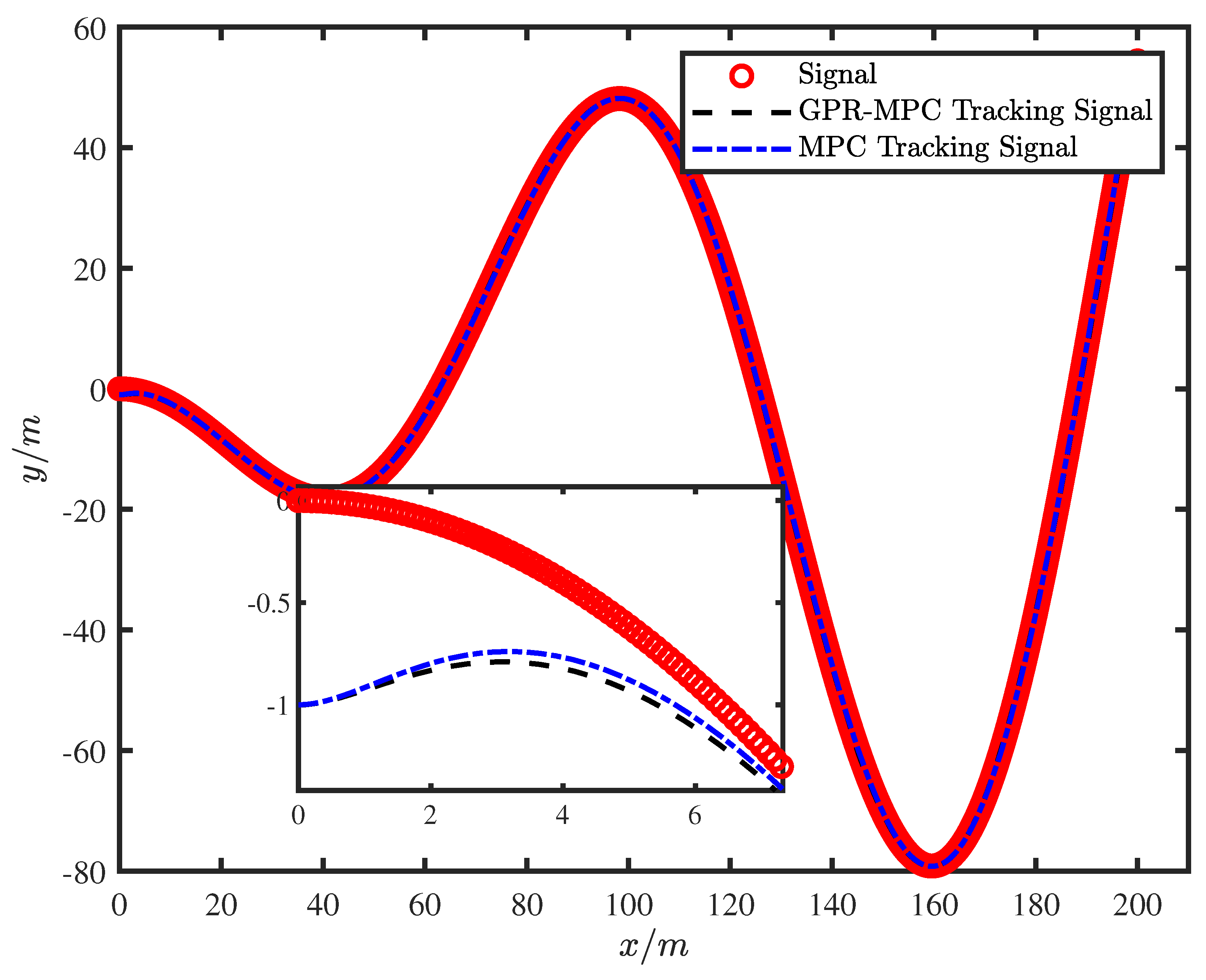
Figure 3 shows the track tracking status of the robot in the $xoy$ plane under different control strategies. It reflects the relationship between the actual position of the wheels and the reasonable position during the track tracking process. From the trajectory tracking curves, it can be seen that the trajectory tracking performance of GPR-MPC algorithm is better in the $XY$ plane and $\theta$ direction, and it can reach the steady state faster, and the difference between the actual position trajectory of the robot and the desired trajectory is smaller. Compared with MPC, the GPR-MPC algorithm has less error.

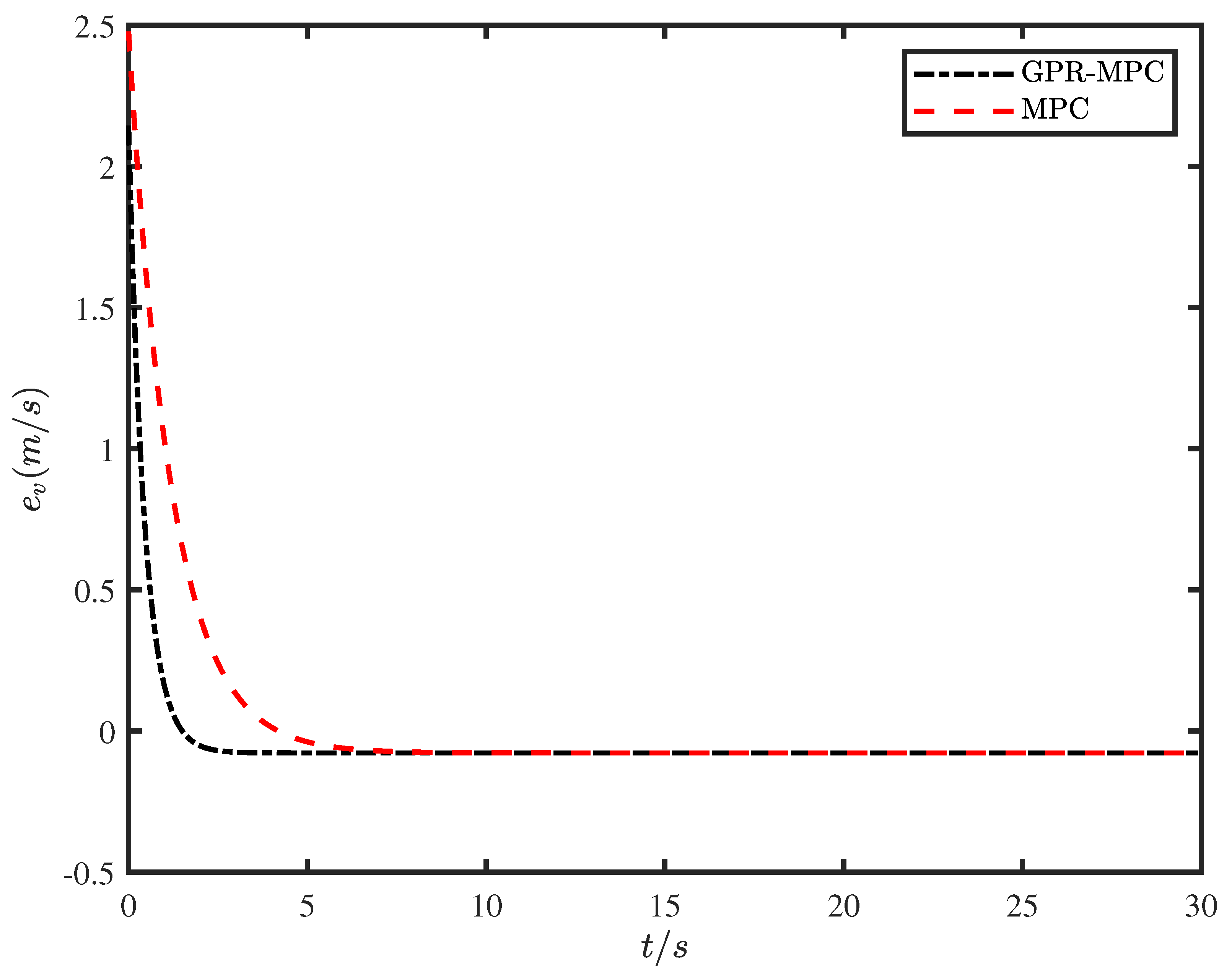
Figure 4 shows the velocity real-time position tracking tracking error under GPR-MPC and MPC control strategies. Since GPR-MPC keeps the cost function in the controller at a minimum value during each control cycle, the optimal control signal is computed to ensure the minimization of the error state. the GPR-MPC controller can force the mobile robot to complete the path tracking task with linearly increasing directional angles. The steady-state tracking error of the velocity is kept within 0.07 under GPR-MPC control, which is obviously well controlled. The results show that GPR-MPC has good performance with fast convergence and sufficiently small steady-state error.

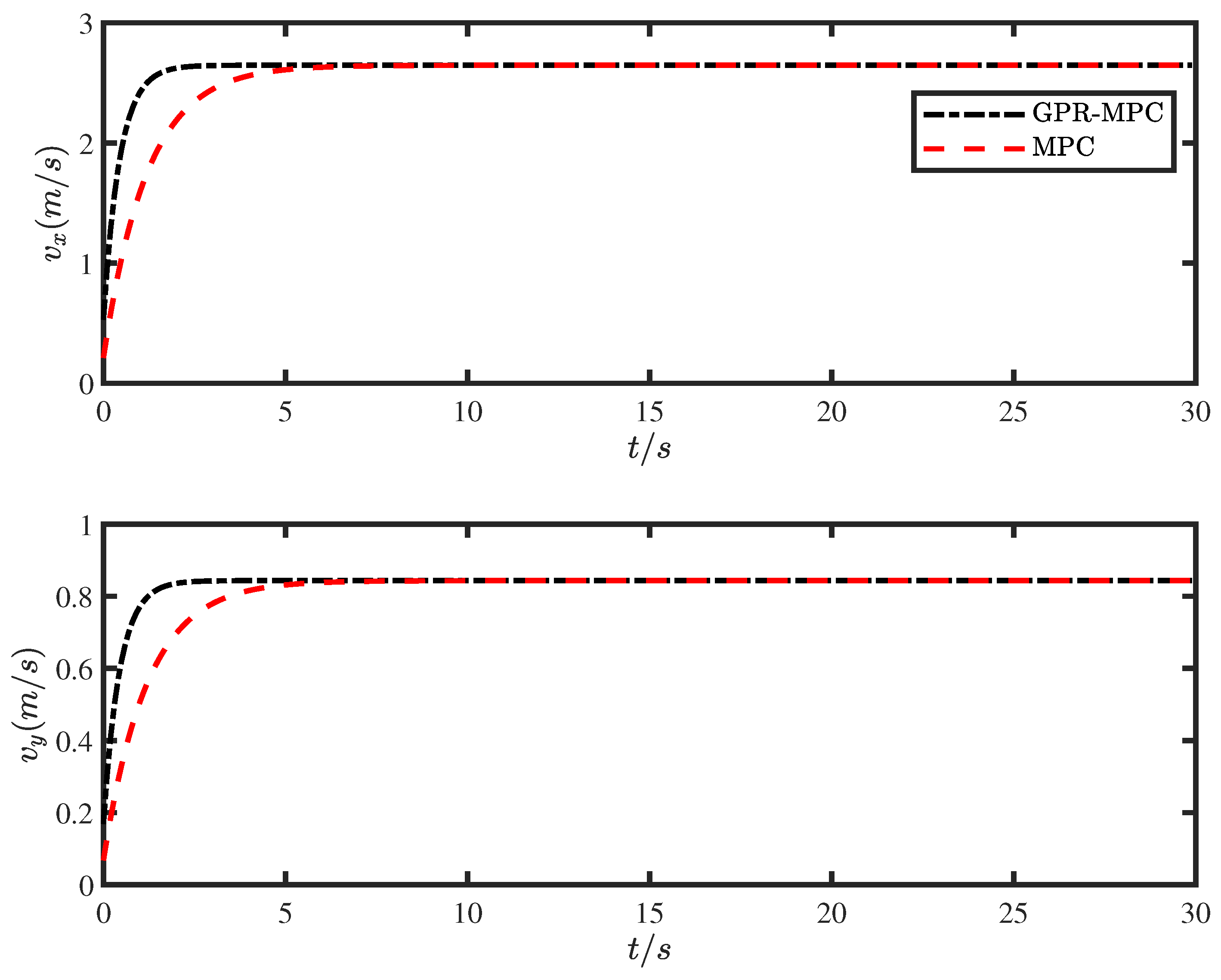
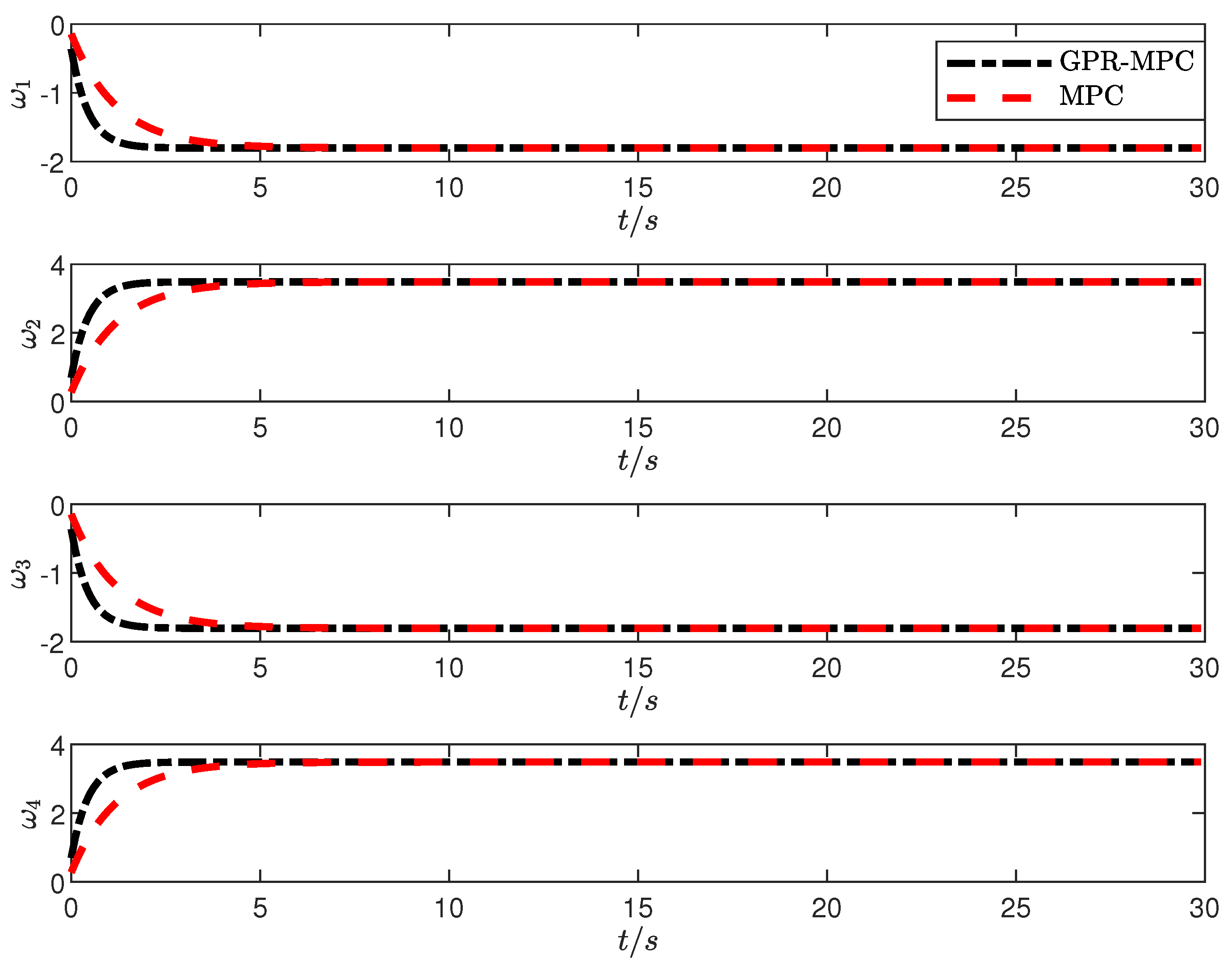
The curves of the velocity component response on $xy$ during the trajectory tracking of the mobile robot with the angular velocity response of the four actuators under the GPR-MPC and MPC control strategies are shown in Figure 5 and Figure 6. As can be seen from the figure, under the GPR-MPC control strategy, the maximum deviation of the GPR-MPC algorithm in the start-up stage is very small, and the time required for the mobile robot to reach the steady state is much smaller than that of the MPC. Under the GPR-MPC control strategy, the velocity along the X and Y axes rises rapidly, reaching a predetermined value of about two seconds. By comparison, the MPC algorithm costs about five seconds. At the same time, under the GPR-MPC control strategy, the speed of the mobile robot reaches the predetermined value stably with small fluctuation and error fluctuation, and the whole control process is relatively stable.

7. Conclusions

In this paper, we establish a dynamic model of the movement of a mobile robot, and then use the model predictive controller to control the system. A GPR-MPC algorithm is proposed to solve the deviation between the model and the actual mobile robot dynamics. The deviation between model prediction and actual dynamics is learned by using GPR in the controller. The controller can perform accurate trajectory tracking with random disturbances and modeling errors. Therefore, it can adapt to unexpected changes such as movement obstacles and inaccuracies in the model. The proposed GPR-MPC mobile robot trajectory tracking control algorithm is more stable and can achieve the desired tracking faster. The speed and RPM response converges quickly to zero and stabilizes in about two seconds. For future research, we suggest the following: (1) Test the controller on real robots; (2) Add more complex targets, such as moving targets; (3) It should also be noted that, due to the introduction of Gaussian process learning, the current learning-based MPC becomes more difficult in calculation, the real-time calculation speed needs to be improved, and some problems need to be solved to implement the above algorithm on the actual robot.

References

- Li, D.; Ye, J. Adaptive robust control of wheeled mobile robot with uncertainties. In Proceedings of the 2014 IEEE 13th International Workshop on Advanced Motion Control (AMC), Yokohama, Japan, 14–16 March 2014; pp. 518–523. [Google Scholar] [CrossRef]
- Alakshendra, V.; Chiddarwar, S. Adaptive robust control of Mecanum-wheeled mobile robot with uncertainties. Nonlinear Dyn. 2017, 87, 2147–2169. [Google Scholar] [CrossRef]
- Zijie, N.; Qiang, L.; Yongjie, C.; Yongjie, C. Fuzzy Control Strategy for Course Correction of Omnidirectional Mobile Robot. Int. J. Control Autom. Syst. 2019, 17, 2354–2364. [Google Scholar] [CrossRef]
- Hendzel, Z.; Rykala, L. Modelling of Dynamics of a Wheeled Mobile Robot with Mecanum Wheels with the use of Lagrange Equations of the Second Kind. Int. J. Appl. Mech. Eng. 2017, 22, 81–99. [Google Scholar] [CrossRef]
- Qian, J.; Zi, B.; Wang, D.; Ma, Y.; Zhang, D. The Design and Development of an Omni-Directional Mobile Robot Oriented to an Intelligent Manufacturing System. Sensors 2017, 17, 2073. [Google Scholar] [CrossRef]
- Baek, J.; Jin, M.; Han, S. A New Adaptive Sliding-Mode Control Scheme for Application to Robot Manipulators. IEEE Trans. Ind. Electron. 2016, 63, 3628–3637. [Google Scholar] [CrossRef]
- Shen, K.; Wang, M.; Fu, M.; Yang, Y.; Yin, Z. Observability Analysis and Adaptive Information Fusion for Integrated Navigation of Unmanned Ground Vehicles. IEEE Trans. Ind. Electron. 2020, 67, 7659–7668. [Google Scholar] [CrossRef]
- Chen, J.; Shuai, Z.; Zhang, H.; Zhao, W. Path Following Control of Autonomous Four-Wheel-Independent-Drive Electric Vehicles via Second-Order Sliding Mode and Nonlinear Disturbance Observer Techniques. IEEE Trans. Ind. Electron. 2021, 68, 2460–2469. [Google Scholar] [CrossRef]
- Yuan, Z.; Tian, Y.; Yin, Y.; Wang, S.; Liu, J.; Wu, L. Trajectory tracking control of a four mecanum wheeled mobile platform: An extended state observer-based sliding mode approach. IET Control. Theory Appl. 2020, 14, 415–426. [Google Scholar] [CrossRef]
- Nguyen, A.T.; Rath, J.; Guerra, T.M.; Palhares, R.; Zhang, H. Robust Set-Invariance Based Fuzzy Output Tracking Control for Vehicle Autonomous Driving Under Uncertain Lateral Forces and Steering Constraints. IEEE Trans. Intell. Transp. Syst. 2021, 22, 5849–5860. [Google Scholar] [CrossRef]
- Yakub, F.; Mori, Y. Comparative study of autonomous path-following vehicle control via model predictive control and linear quadratic control. Proc. Inst. Mech. Eng. Part D J. Automob. Eng. 2015, 229, 1695–1714. [Google Scholar] [CrossRef]
- Luo, Q.; Nguyen, A.T.; Fleming, J.; Zhang, H. Unknown Input Observer Based Approach for Distributed Tube-Based Model Predictive Control of Heterogeneous Vehicle Platoons. IEEE Trans. Veh. Technol. 2021, 70, 2930–2944. [Google Scholar] [CrossRef]
- Cao, M.; Hu, C.; Wang, R.; Wang, J.; Chen, N. Compensatory model predictive control for post-impact trajectory tracking via active front steering and differential torque vectoring. Proc. Inst. Mech. Eng. Part D J. Automob. Eng. 2021, 235, 903–919. [Google Scholar] [CrossRef]
- Amidi, O. Integrated Mobile Robot Control. Proc. SpieInt. Soc. Opt. Eng. 1990, 91, 504–523. [Google Scholar] [CrossRef]
- Rasekhipour, Y.; Khajepour, A.; Chen, S.K.; Litkouhi, B. A Potential Field-Based Model Predictive Path-Planning Controller for Autonomous Road Vehicles. IEEE Trans. Intell. Transp. Syst. 2017, 18, 1255–1267. [Google Scholar] [CrossRef]
- Ji, J.; Khajepour, A.; Melek, W.W.; Huang, Y. Path Planning and Tracking for Vehicle Collision Avoidance Based on Model Predictive Control With Multiconstraints. IEEE Trans. Veh. Technol. 2017, 66, 952–964. [Google Scholar] [CrossRef]
- Kim, J.C.; Pae, D.S.; Lim, M.T. Obstacle Avoidance Path Planning Algorithm Based on Model Predictive Control. In Proceedings of the 2018 18th International Conference on Control, Automation and Systems (ICCAS), PyeongChang, Republic of Korea, 17–20 October 2018; pp. 141–143. [Google Scholar]
- Guo, Hongyan and Cao, Dongpu and Chen, Hong and Sun, Zhenping and Hu, Yunfeng Model predictive path following control for autonomous cars considering a measurable disturbance: Implementation, testing, and verification. Mech. Syst. Signal Process. 2019, 118, 41–60. [CrossRef]
- Xu, W.; Chen, R.T.Q.; Li, X.; Duvenaud, D. Infinitely Deep Bayesian Neural Networks with Stochastic Differential Equations. In Proceedings of the Proceedings of the 25th International Conference on Artificial Intelligence and Statistics, Valencia, Spain, 28–30 March 2022; Volume 151, pp. 721–738. [Google Scholar] [CrossRef]
- Shen, D. Iterative learning control with incomplete information: A survey. IEEE/CAA J. Autom. Sin. 2018, 5, 885–901. [Google Scholar] [CrossRef]
- Aswani, A.; Gonzalez, H.; Sastry, S.S.; Tomlin, C. Provably Safe and Robust Learning-Based Model Predictive Control. Automatica 2013, 49, 1216–1226. [Google Scholar] [CrossRef]
- Soloperto, R.; Köhler, J.; Allgöwer, F. Augmenting MPC Schemes With Active Learning: Intuitive Tuning and Guaranteed Performance. IEEE Control Syst. Lett. 2020, 4, 713–718. [Google Scholar] [CrossRef]
- Chakrabarty, A.; Dinh, V.; Corless, M.J.; Rundell, A.E.; Żak, S.H.; Buzzard, G.T. Support Vector Machine Informed Explicit Nonlinear Model Predictive Control Using Low-Discrepancy Sequences. IEEE Trans. Autom. Control. 2017, 62, 135–148. [Google Scholar] [CrossRef]
- Benjamin, K.; Sergio, L. Deep learning-based embedded mixed-integer model predictive control. In Proceedings of the 2018 European Control Conference (ECC), Limassol, Cyprus, 12–15 June 2018; pp. 2075–2080. [Google Scholar] [CrossRef]
- Zhang, K.; Sun, Q.; Shi, Y. Trajectory Tracking Control of Autonomous Ground Vehicles Using Adaptive Learning MPC. IEEE Trans. Neural Netw. Learn. Syst. 2021, 32, 5554–5564. [Google Scholar] [CrossRef] [PubMed]
- Karg, B.; Lucia, S. Efficient Representation and Approximation of Model Predictive Control Laws via Deep Learning. IEEE Trans. Cybern. 2020, 50, 3866–3878. [Google Scholar] [CrossRef] [PubMed]
- Tange, Y.; Kiryu, S.; Matsui, T. Model Predictive Control Based on Deep Reinforcement Learning Method with Discrete-Valued Input. In Proceedings of the 2019 IEEE Conference on Control Technology and Applications (CCTA), Hong Kong, China, 19–21 August 2019; pp. 308–313. [Google Scholar] [CrossRef]
- Karg, B.; Lucia, S. Approximate moving horizon estimation and robust nonlinear model predictive control via deep learning. Comput. Chem. Eng. 2021, 148, 107266. [Google Scholar] [CrossRef]
- Perez, E.A.M.; Iba, H. Deep Learning-Based Inverse Modeling for Predictive Control. IEEE Control. Syst. Lett. 2022, 6, 956–961. [Google Scholar] [CrossRef]
- Datta, A.; Augustin, M.J.; Gupta, N.; Viswamurthy, S.R.; Gaddikeri, K.M.; Sundaram, R. Impact Localization and Severity Estimation on Composite Structure Using Fiber Bragg Grating Sensors by Least Square Support Vector Regression. IEEE Sens. J. 2019, 19, 4463–4470. [Google Scholar] [CrossRef]
- Klenske, E.D.; Zeilinger, M.N.; Schölkopf, B.; Hennig, P. Gaussian Process-Based Predictive Control for Periodic Error Correction. IEEE Trans. Control Syst. Technol. 2016, 24, 110–121. [Google Scholar] [CrossRef]
- Janssen, N.H.J.; Kools, L.; Antunes, D.J. Embedded Learning-based Model Predictive Control for Mobile Robots using Gaussian Process Regression. In Proceedings of the 2020 American Control Conference (ACC), Denver, CO, USA, 1–3 July 2020; pp. 1124–1130. [Google Scholar] [CrossRef]
- Cao, M.; Wang, R.; Chen, N.; Wang, J. A Learning-Based Vehicle Trajectory-Tracking Approach for Autonomous Vehicles With LiDAR Failure Under Various Lighting Conditions. IEEE/Asme Trans. Mechatron. 2022, 27, 1011–1022. [Google Scholar] [CrossRef]
- Hewing, L.; Kabzan, J.; Zeilinger, M.N. Cautious Model Predictive Control Using Gaussian Process Regression. IEEE Trans. Control Syst. Technol. 2020, 28, 2736–2743. [Google Scholar] [CrossRef]
- Bonzanini, A.D.; Paulson, J.A.; Makrygiorgos, G.; Mesbah, A. Fast approximate learning-based multistage nonlinear model predictive control using Gaussian processes and deep neural networks. Comput. Chem. Eng. 2021, 145, 107174. [Google Scholar] [CrossRef]
Figure 1.
Schematic diagram of mobile robot mechanism.
Figure 2.
MPC Block Diagram.
Figure 3.
Mobile robot track tracking position status.
Figure 4.
Mobile robot trajectory tracking error.
Figure 5.
Mobile robot trajectory tracking speed.
Figure 6.
Mobile robot trajectory speed response.