Using High-Order Particle Velocity Gradient Polarization Characteristics to Detect Underwater Coherent Interference

Abstract

Detection of underwater coherent interference is necessary as its presence affects the estimation of the desired target. In this work, a method based on high-order particle velocity gradient polarization characteristics is proposed to distinguish the presence of coherent interference. Characteristics including ellipse ratio and inclination angles of the high-order particle velocity gradient are chosen as effective detection features because they remain unchanged at different orders of the desired target but changed at different orders of coherent signals when there is coherent interference. Based on such altered properties, a quick and effective marine detection system can be established. Both simulation and experimental results validate the proposed detection method.

1. Introduction

Coherent jammers in marine electronic warfare systems can generate signals that are coherent with the desired signal, even when the signals approach the hydrophones from different directions [1]. They can degrade the performance of underwater adaptive array system direction finding algorithms. In actuality, coherent signals appear to be a single signal impinging on the hydrophones and arriving from a completely different direction than the desired signals [2]. Detecting the underwater coherent jammers is crucial for taking additional precautions [3]. In the following, the research progress in the fields of polarization and high-order particle velocity gradients are illustrated in order to introduce the high-order particle velocity gradient polarization characteristic proposed in this study.

Polarization is a feature common to all vector signals that describe the time-varying space trajectories of vector endpoints at a fixed point in wave propagation space. Wave polarization is a hot topic in many fields, including electromagnetism [4,5] and geophysics [6,7,8]. With the further study of polarization, the concept was introduced into acoustics [9,10]. The coherence function between acoustic pressure and particle velocity and the curl of active intensity are proposed as two indicators for estimating the degree of coherence and the polarization of acoustic fields [11]. Because of energy oscillations due to the instantaneous reactive intensity, a kind of energy polarization is shown to occur in certain acoustic fields [12]. In recent years, polarization has also been widely used in underwater acoustics. The Stokes parameter framework was presented by Bonnel [13], it enables a description of the polarization of the underwater acoustic field. It differs from other underwater vector acoustic works in that it focuses exclusively on the particle velocity v rather than on the complex intensity I = pv*, which requires a concurrent and collocated measure of both pressure p and particle velocity v. We also only use particle velocity in the acoustic field. Moreover, the Stokes parameter framework is used by Dahl [14] to help obtain the circularity and degree of polarization, clearly demonstrating properties of bivariate signal trajectory. We also use the characteristics of circularity. Shchurov [15] hypothesized that when measuring a single plane wave field, the incident acoustic wave is a single longitudinal wave. When two incident plane waves of identical frequency coexist, the particle velocity is a rotation vector, and the trajectory at the end of the vector is an ellipse. We have conducted exhaustive research to address the following case: when the phase difference between the desired target and coherent interference signals is 0 and π, the trajectory turns into a straight line. To solve this problem, we propose employing high-order particle velocity polarization characteristics.

The emergence of vector sensors has allowed the scalar information processing of the sound pressure to the vector information processing of the particle velocity [16]. The high-order particle velocity gradient sensor makes it possible for vector hydrophones to achieve better performance [17].

For decades, high-order acoustic vector sensors and their array processing technology have been a hot topic in underwater acoustic engineering. High-order hydrophones provide a novel approach to underwater acoustic problem solving [18,19]. The concept of high-order hydrophones was first proposed in 1992 by Spain [20], carried out by Taylor series expansion of sound pressure in a limited region. The results showed the relationship between sound pressure, sound pressure gradient and particle velocity; the idea of using the second-order gradient of sound pressure was proposed to improve the directivity of the acoustic array. In 1999, Bastyr used a neutral buoyant u-u sound intensity probe [21] to measure the particle velocity at two adjacent points; it was the first attempt to measure the particle velocity gradient in water. In 2001, M.T. Silvia [22] successfully used a vector sensor and measured the directivity of ${\cos }^2\theta$ and ${\sin }^2\theta$. In 2003, Cray [23] and others deduced the Taylor series expansion of the sound pressure at the origin of the Cartesian coordinate system, pointing out that the first-order sound pressure gradient is proportional to the particle velocity, the second-order sound pressure gradient is proportional to the first-order particle velocity gradient, and the spatial pure partial derivative of the particle velocity component is proportional to the instantaneous density of the sound field.

With more and more indepth research on high-order sensors, a number of scholars have focused on the acquisition and optimization of a high-order gradient model to obtain better high-order application. Schmidlin introduced a generalized function approach for estimating spatial partial derivatives of pressure [24]. This approach was utilized to develop a theoretical scheme for implementing directional acoustic sensors of an arbitrary order. Explicit formulas were found for the filter coefficients that maximize the array gain of the filter and establish an explicit expression for the maximum array gain [25]. A linear prediction model was used to write the high-order derivatives in terms of the lower order derivatives, which was then used to estimate the high-order spatial derivatives [26]. Using the high-order derivatives, the signal can be extrapolated over a larger aperture. A subtractive beamform for short vector hydrophone arrays was presented based on the extraction of the directional modes of the acoustic field from finite difference-based approximations of the particle velocity gradients [27].

In this paper, a new method using high-order particle velocity gradient polarization characteristics to distinguish whether there is coherent interference is proposed. Firstly, the particle velocity polarization characteristics of a single target and multiple coherent signals are deduced theoretically. The result shows that the particle velocity gradient polarization trajectories under the condition of a single target are all straight lines, and the particle velocity gradient polarization trajectories under the condition of multiple coherent signals are ellipses. Then, we take the case of two coherent signals as an example; it is found that when the phase difference between them is 0° and 180°, the trajectories are all straight lines and cannot be separated. Further, the use of high-order particle velocity polarization characteristics can not only solve the problem in the above special case, but also distinguish the case of a single target and multiple coherent signals through increasing the polarization characteristics dimension. The results show that both the simulation and the experiment results in the presence of noise achieve the aim of distinguishing one and multiple targets.

The rest of this article is arranged as follows: Section 2 lays the theoretical foundation, providing the theoretical deduction of the particle velocity polarization characteristics and high-order particle velocity gradient polarization characteristics. In Section 3, we explore polarization characteristics under different target conditions. A BP neural network is used for recognition, and the recognition effect is specified. In Section 4, an experiment using a single target and coherent signals signal is carried out in an anechoic water pool, and the test results are analyzed to show the feasibility of the proposed features. Finally, conclusions are provided in Section 5.

2. Materials and Methods

2.1. Particle Velocity Polarization Characteristics of a Marine Target

Suppose that a far-field narrowband signal impinges on a vector hydrophone, the two-dimensional situation is considered, and the output of the vector hydrophone can be expressed as follows [27]:

$$\begin{array}{l}{v}_x=V\cos \varphi {\mathrm{e}}^{\mathrm{j}\omega \mathrm{t}};\\ v_y=V\sin \varphi {\mathrm{e}}^{\mathrm{j}\omega \mathrm{t}};\end{array}$$

(1)

where $V$ is the amplitude of the velocity field variable, $\omega$ is the angular frequency, and $\varphi$ is the incident angle of the target, which is measured counterclockwise from the x-axis.

The displacement component of this position can be expressed as

$$\begin{array}{l}{u}_x=\mathrm{real}({\displaystyle \int v_{x}dt})=V\cos \varphi \frac{\sin \omega t}{\omega };\\ u_y=\mathrm{real}({\displaystyle \int v_{y}dt})=V\sin \varphi \frac{\sin \omega t}{\omega };\end{array}$$

(2)

The particle motion equation is given as $\frac{u_y}{u_x}=\tan \varphi$. The particle trajectory is a line with $\tan \varphi$ slope. The polarization characteristics of a marine target are that the length of the major axis L_A is $V/\omega$, the length of the minor axis S_A is 0, the inclination of the line $\tau$, which is defined as the angle between the major axis and the +x axis, is the incident angle $\varphi$. The ellipse ratio angle $\epsilon$ is defined as the smallest interior angle in a right triangle with the major and minor axes of the ellipse as sides is 0°.

2.2. Particle Velocity Polarization Characteristics of Multiple Coherent Signals

In the presence of multiple coherent interferences in the marine acoustic field, the particle velocity v_c received at a point in space is defined as [28]

$$\begin{array}{l}{v}_{cx}=V\cos \varphi {\mathrm{e}}^{\mathrm{j}\omega t}+{\displaystyle \sum _i{V}_i\cos {\varphi }_i{\mathrm{e}}^{\mathrm{j}(\omega t+{\phi }_i)}}\\ v_{cy}=V\sin \varphi {\mathrm{e}}^{\mathrm{j}\omega t}+{\displaystyle \sum _i{V}_i\sin {\varphi }_i{\mathrm{e}}^{\mathrm{j}(\omega t+{\phi }_i)}}\end{array},$$

(3)

where $v_{cx}$ and $v_{cy}$ are the components of the particle velocity $v_c$. $i$ denotes the number of the coherent interference; $V_i$ is the amplitude of each coherent interference; ${\varphi }_i$ is the incident angle of multiple coherent interference, and the phase difference between the desired target signal source and the coherent interference signal is ${\phi }_i$. The displacement component of this position can be expressed as

$$u_c=\mathrm{real}{\displaystyle \int v_{c}dt}=\left[\begin{array}{c}V\cos \varphi \frac{\sin \omega t}{\omega }+{\displaystyle \sum _i{V}_i\cos {\varphi }_i\frac{\sin (\omega t+{\phi }_i)}{\omega }}\\ V\sin \varphi \frac{\sin \omega t}{\omega }+{\displaystyle \sum _i{V}_i\sin {\varphi }_i\frac{\sin (\omega t+{\phi }_i)}{\omega }}\end{array}\right].$$

(4)

We select two coherent signals (the desired target and a coherent interference) as an example.

$$v_c=V\left[\begin{array}{c}\cos \varphi \\ \sin \varphi \end{array}\right]{\mathrm{e}}^{\mathrm{j}\omega \mathrm{t}}+V_1\left[\begin{array}{c}\cos {\varphi }_1\\ \sin {\varphi }_1\end{array}\right]{\mathrm{e}}^{\mathrm{j}(\omega \mathrm{t}+{\phi }_1)},$$

(5)

$$u_c=V\left[\begin{array}{c}\cos \varphi \\ \sin \varphi \end{array}\right]\frac{\sin (\omega t)}{\omega }+V_1\left[\begin{array}{c}\cos {\varphi }_1\\ \sin {\varphi }_1\end{array}\right]\frac{\sin (\omega t+{\phi }_1)}{\omega }=\left[\begin{array}{c}{A}_{mx}\sin \left(\omega t+\arctan p_{hx}\right)\\ A_{my}\sin \left(\omega t+\arctan p_{hy}\right)\end{array}\right],$$

(6)

where

$$A_{mx}=\frac{\sqrt{{\left(V\cos \varphi +V_1\cos {\varphi }_1\cos {\phi }_1\right)}^2+{\left(V_1\cos {\varphi }_1\sin {\phi }_1\right)}^2}}{\omega },$$

(7)

$$A_{my}=\frac{\sqrt{{\left(V\sin \varphi +V_1\sin {\varphi }_1\cos {\phi }_1\right)}^2+{\left(V_1\sin {\varphi }_1\sin {\phi }_1\right)}^2}}{\omega },$$

(8)

$$p_{hx}=\arctan \frac{V_1\cos {\varphi }_1\sin {\phi }_1}{V\cos \varphi +V_1\cos {\varphi }_1\cos {\phi }_1},$$

(9)

$$p_{hy}=\arctan \frac{V_1\sin {\varphi }_1\sin {\phi }_1}{V\sin \varphi +V_1\sin {\varphi }_1\cos {\phi }_1}.$$

(10)

The particle motion equation is

$$\frac{u_x^2}{A_{mx}^2}+\frac{u_y^2}{A_{my}^2}-2\frac{u_x}{A_{mx}}\frac{u_y}{A_{my}}\cos \left(p_{hy}-p_{hx}\right)={\sin }^2\left(p_{hy}-p_{hx}\right).$$

(11)

It can be seen from the equation that when there are two coherent signals, the particle trajectory is an ellipse.

However, when $\sin {\phi }_1=0$ or $\sin (\varphi -{\varphi }_1)=0$, the particle trajectory of the two coherent signals is a straight line. Because the trigonometric function is periodic, we divided it into four cases to discuss the case where the particle trajectories of two coherent signals are straight lines: $\varphi ={\varphi }_1$, $\varphi -{\varphi }_1=180°$, ${\phi }_1=0°$ and ${\phi }_1=180°$. When $\varphi ={\varphi }_1$, i.e., the two coherent signals are each incident at a target, there is no need to distinguish between them. In practical applications, because of the influence of the ocean environment, the target cannot always be on the line of the incident angle of two coherent signals; thus, when the incident signal is $\varphi -{\varphi }_1=180°$, we can obtain the variation of the particle trajectory over time.

The phase difference between two coherent signals is 0° and 180° by introducing the high-order particle velocity gradient polarization characteristics to distinguish two coherent signals from a single target. Furthermore, through the introduction of the high-order particle velocity gradient polarization characteristics, the dimension of polarization characteristics can be increased, so that a single target and two coherent signals can be better distinguished.

2.3. High-Order Particle Velocity Gradient Polarization Characteristics of a Marine Target

The nth-order particle velocity gradient of a target given at $x=0$ is defined as [27]

$$\begin{array}{l}{v}_x{}^{(n)}=\frac{{\partial }^n{v}_x}{\partial x^n}\left|{}_{x=0}\right.=V{(\mathrm{j}k)}^n{\cos }^{n+1}\varphi {\mathrm{e}}^{\mathrm{j}\omega \mathrm{t}};\\ v_y{}^{(n)}=\frac{{\partial }^n{v}_y}{\partial x^n}\left|{}_{x=0}\right.=V{(\mathrm{j}k)}^n\sin \varphi {\cos }^n\varphi {\mathrm{e}}^{\mathrm{j}\omega \mathrm{t}}\end{array}.$$

(12)

where j is the imaginary unit, and k is the wavenumber.

The nth order of the displacement component of this position can be expressed as

$$\begin{array}{l}{u}_x{}^{(n)}=\mathrm{real}({\displaystyle \int v_x{}^{(n)}dt})=\left\{\begin{array}{l}\frac{k^n{\mathrm{j}}^{n}V{\left(\cos \varphi \right)}^{n+1}\sin \left(\omega t\right)}{\omega }\left(n \mathrm{even}\right)\\ \frac{k^n{\mathrm{j}}^{n-1}V{\left(\cos \varphi \right)}^{n+1}\cos \left(\omega t\right)}{\omega }\left(n \mathrm{odd}\right)\end{array}\right.\\ u_y{}^{(n)}=\mathrm{real}({\displaystyle \int v_y{}^{(n)}dt})=\left\{\begin{array}{l}\frac{k^n{\mathrm{j}}^{n}V\sin \varphi {\left(\cos \varphi \right)}^n\sin \left(\omega t\right)}{\omega }\left(n \mathrm{even}\right)\\ \frac{k^n{\mathrm{j}}^{n-1}V\sin \varphi {\left(\cos \varphi \right)}^n\cos \left(\omega t\right)}{\omega }\left(n \mathrm{odd}\right)\end{array}\right.;\end{array}.$$

(13)

The particle motion equation is $u_y{}^{(n)}/u_x{}^{(n)}=\tan \varphi$. The trajectories of each order of the particle velocity gradient are all straight lines. The polarization characteristics of a target for each order are such that the length of the major axis L_A is the maximum distance between a point and the origin in the trajectory. The length of the minor axis S_A is 0. The ellipse inclination angle is also the incident angle, and the ellipse ratio angle is 0°.

When there is a single target, the characteristics of particle velocity and nth-order particle velocity gradient are shown in

Table 1. Particle velocity and nth-order particle velocity gradient polarization characteristics of a marine target.

A Target	LA	SA	Inclination Angle	Ratio Angle
Particle velocity	different	same	same	same
Nth-order particle velocity

. It is clear that the unchanged characteristics for S_A are all 0, the ellipse inclination angle is also the incident angle, and the ellipse ratio angle is 0°.

2.4. High-Order Particle Velocity Gradient Polarization Characteristics of Multiple Coherent Signals

In the presence of multiple coherent interferences in the ocean, the high-order particle velocity gradient $v_{cx}{}^{(n)}$ can be derived from Formulas (3) and (12),

$$\begin{array}{l}{v}_{cx}{}^{(n)}=\frac{{\partial }^n{v}_{cx}}{\partial x^n}=V{\cos }^n\varphi {\mathrm{e}}^{\mathrm{j}\omega t}+{\displaystyle \sum _i{V}_i{\cos }^n{\varphi }_i{\mathrm{e}}^{\mathrm{j}(\omega t+{\phi }_i)}}\\ v_{cy}{}^{(n)}=\frac{{\partial }^n{v}_{cy}}{\partial x^n}=V\sin \varphi {\cos }^n\varphi {\mathrm{e}}^{\mathrm{j}\omega t}+{\displaystyle \sum _i{V}_i\sin {\varphi }_i{\cos }^n{\varphi }_i{\mathrm{e}}^{\mathrm{j}(\omega t+{\phi }_i)}}\end{array}.$$

(14)

The displacement component of this position can be expressed as

$$u_c{}^{(n)}=\mathrm{real}{\displaystyle \int v_c{}^{(n)}dt}=\left[\begin{array}{c}V{\cos }^n\varphi \frac{\sin \omega t}{\omega }+{\displaystyle \sum _i{V}_i{\cos }^n{\varphi }_i\frac{\sin (\omega t+{\phi }_i)}{\omega }}\\ V\sin \varphi {\cos }^n\varphi \frac{\sin \omega t}{\omega }+{\displaystyle \sum _i{V}_i\sin {\varphi }_i{\cos }^n{\varphi }_i\frac{\sin (\omega t+{\phi }_i)}{\omega }}\end{array}\right].$$

(15)

We also select two coherent signals (the desired target and a coherent interference) as an example.

$$v_c{}^{(n)}=V\left[\begin{array}{c}{\cos }^n\varphi \\ \sin \varphi {\cos }^n\varphi \end{array}\right]{\mathrm{e}}^{\mathrm{j}\omega \mathrm{t}}+V_1\left[\begin{array}{c}{\cos }^n{\varphi }_1\\ \sin {\varphi }_1{\cos }^n{\varphi }_1\end{array}\right]{\mathrm{e}}^{\mathrm{j}(\omega \mathrm{t}+{\phi }_1)},$$

(16)

$$u_c{}^{(n)}=V\left[\begin{array}{c}{\cos }^n\varphi \\ \sin \varphi {\cos }^n\varphi \end{array}\right]\frac{\sin (\omega t)}{\omega }+V_1\left[\begin{array}{c}{\cos }^n{\varphi }_1\\ \sin {\varphi }_1{\cos }^n{\varphi }_1\end{array}\right]\frac{\sin (\omega t+{\phi }_1)}{\omega }=\left[\begin{array}{c}{A}_{nmx}\sin \left(\omega t+p_{nhx}\right)\\ A_{nmy}\sin \left(\omega t+p_{nhy}\right)\end{array}\right].$$

(17)

where

$$A_{nmii}=\frac{k^n\sqrt{a_{nii}{}^2+a_{nii1}{}^2+2a_{nii}{a}_{nii1}\cos {\phi }_1}}{\omega };$$

(18)

$$p_{nhii}=\left\{\begin{array}{l}\arctan \left(\frac{a_{nii1}\sin {\phi }_1}{a_{nii}+a_{nii1}\cos {\phi }_1}\right) \left(n \mathrm{even}\right)\\ \arctan \left(-\frac{a_{nii}+a_{nii1}\cos {\phi }_1}{a_{nii1}\sin {\phi }_1}\right) \left(n \mathrm{odd}\right)\end{array}\right.,$$

(19)

where ii denotes x and y axis component, $a_{nx}=V{\cos }^{n+1}\varphi ;a_{nx1}=V_1{\cos }^{n+1}{\varphi }_1$ $a_{ny}=V\sin \varphi {\cos }^n\varphi ;a_{ny1}=V_1\sin {\varphi }_1{\cos }^n{\varphi }_1$

The particle motion equation is

$$\frac{u_x^{{\left(n\right)}^2}}{A_{nmx}^2}+\frac{u_y^{{\left(n\right)}^2}}{A_{nmy}^2}-2\frac{u_x^{\left(n\right)}}{A_{nmx}}\frac{u_y^{\left(n\right)}}{A_{nmy}}\cos \left(p_{nhy}-p_{nhx}\right)={\sin }^2\left(p_{nhy}-p_{nhx}\right).$$

(20)

From

Table 2. Particle velocity and nth-order particle velocity gradient polarization characteristics of coherent signals.

Coherent Signals	LA	SA	Inclination Angle	Ratio Angle
Particle velocity	different	different	different	different
Nth-order particle velocity

, it can be seen that in the case of two coherent signals, the different order of particle velocity gradient trajectory is an ellipse. However, the lengths of L_A and S_A, the inclination angle, and the ratio angle of the ellipse are different.

However, when $\sin {\phi }_1=0$, it can be deduced that the polarization trajectories of the two coherent signals are also straight lines. Thus, S_A cannot be the efficient detection characteristic. Let ${\phi }_1=0°$ and ${\phi }_1=180°$ in the particle motion equation. The inclination angle of each order of the high-order particle velocity gradient is $\tau =\arctan \frac{a_{ny}\pm a_{ny1}}{a_n{}_x\pm a_{nx1}}$, where addition is applied when the phase difference is 0° and subtraction is applied when the phase difference is 180°. From the equation, different orders have different inclination angles. However, a single target’s inclination angle is changeless in different order. In this situation, a single target and two coherent signals can still be distinguished by the high-order particle velocity gradient polarization characteristics.

According to the above analysis, we choose the inclination angle and ratio angle of the ellipse of the high-order particle velocity gradient as the polarization characteristics to distinguish between a target and two coherent signals.

The Back-Propagation (BP) neural network is a model in the field of artificial neural networks [29]. It is a multilayer and backpropagation feedforward artificial neural network that achieves a nonlinear mapping between input and output through the error training process for testing the effectiveness of high-order particle velocity gradient polarization characteristics. The high-order particle velocity gradient polarization characteristics, including the ellipse inclination and ratio angles of a single target and two coherent signals from different angles, are the training data. Single target samples with random incident angles and two coherent signals from two random incident angles are the test data for the BP neural network. A single hidden layer network in BP neural network is selected [30]. The number of input layer nodes is the feature dimension, and the number of hidden layer nodes is performed by $m=\sqrt{n+l}+\alpha$ and the number of output layer nodes is 2; where m is the number of hidden layer nodes, n is the number of input layer nodes, l is the number of output layer nodes, and $\alpha$ is the adjusting constant, whose value ranges from 0 to 10.

3. Simulation Results and Analysis

This section presents some simulations to validate the above theoretical derivation. The frequencies of the target and two coherent signals are 1 kHz.

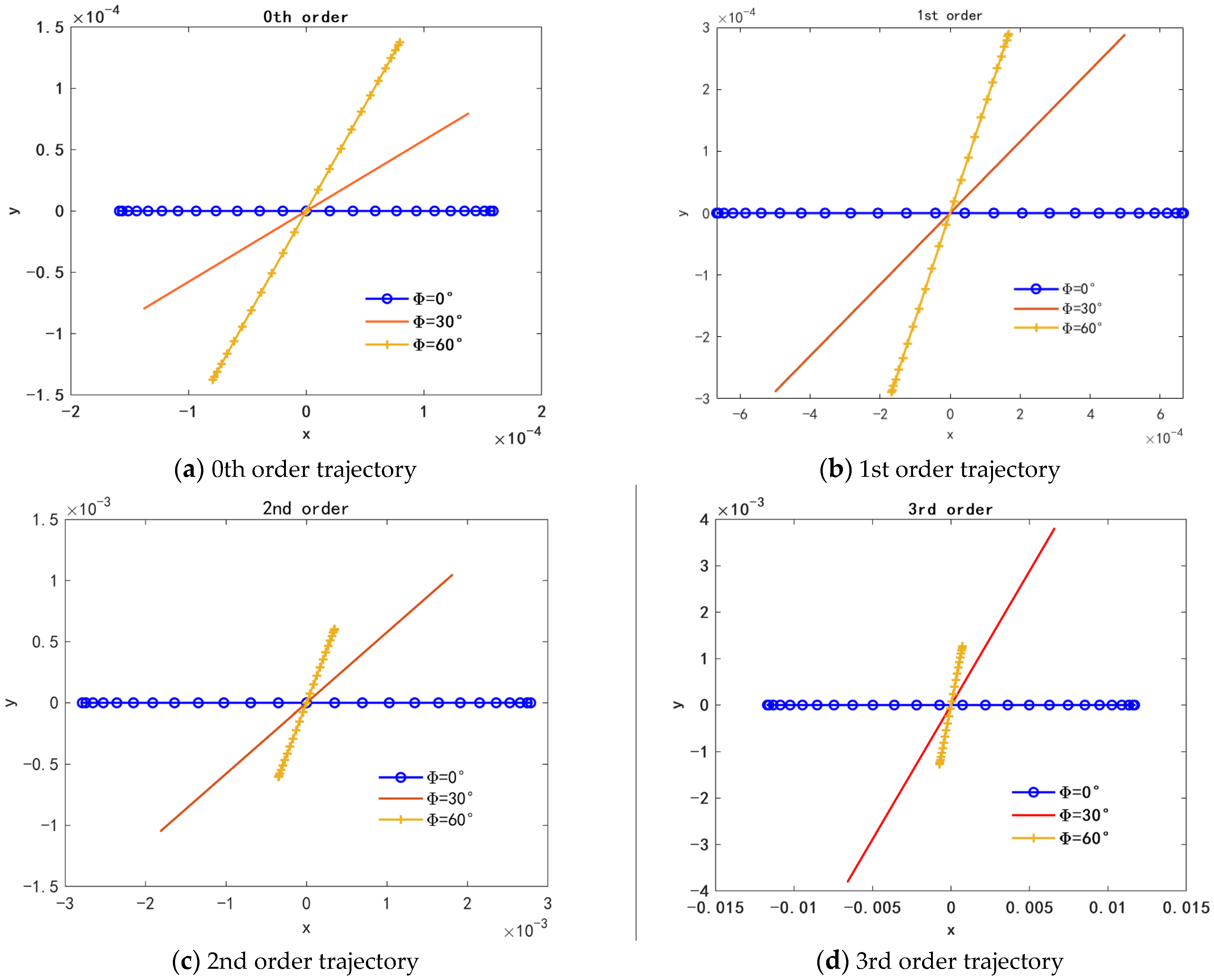
Figure 1 shows the 0th, 1st, 2nd, and 3rd order particle trajectories of a marine target. The incident angles are 0° (o blue line), 30° (red solid line), and 60° (yellow + line), respectively.

It can be seen from Figure 1 that the different order particle velocity gradient polarization trajectories are all straight lines, that is, the ratio angles are all 0°, and the inclination angles are all the same as the incident angles.

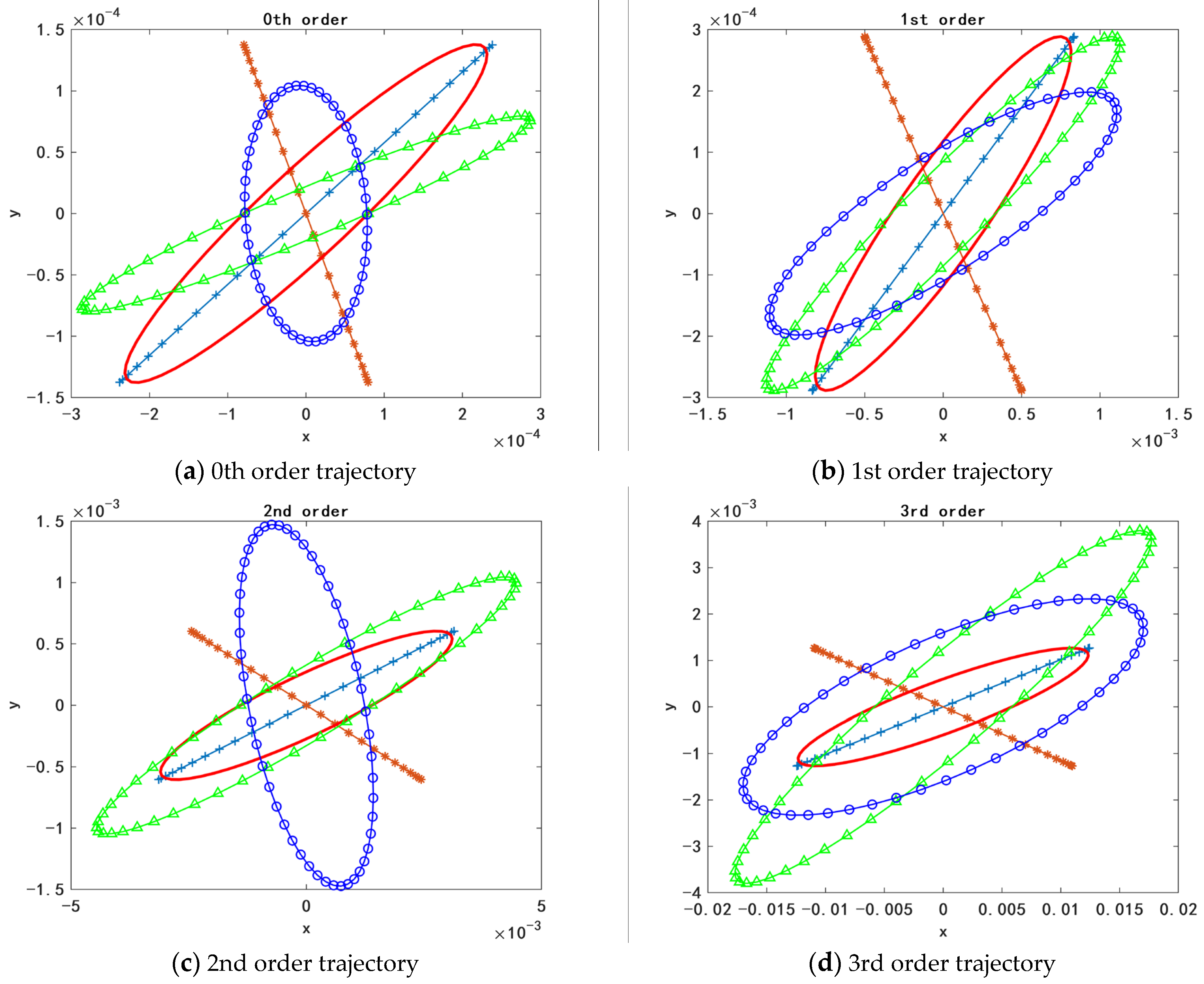
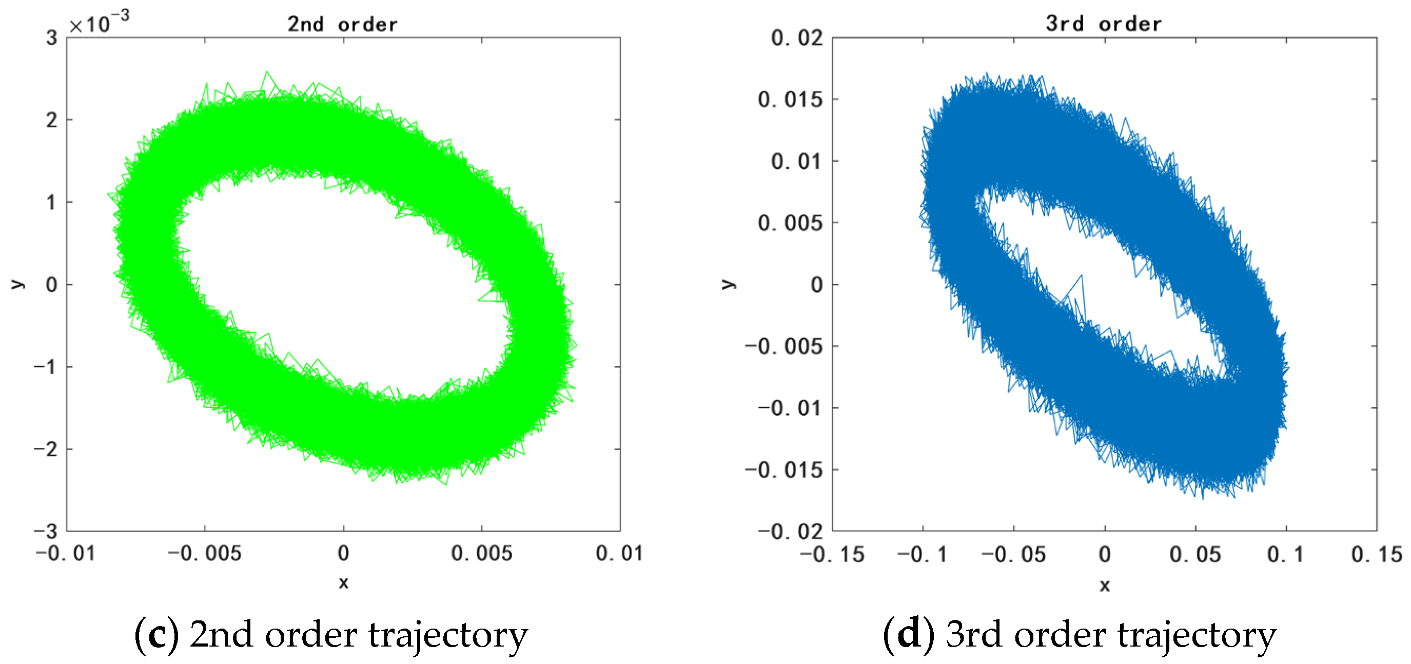
Figure 2 shows the 0th, 1st, 2nd, and 3rd order particle trajectories of two coherent signals. In the case of $\sin {\phi }_1=0$, the incident angles are 0° and 60°, and the phase difference is 0° (+ line) and 180° (* line). When the incident angles are 0° and 60°, the phase difference is 30° (red solid line). When the incident angles are 0° and 30°, the phase difference is 30° (green triangular line). When the incident angles are 30° and 170°, the phase difference is 30° (blue o line).

The blue + line and the red * line in Figure 2 correspond to the case where $\sin {\phi }_1=0$; they are all straight lines, which is consistent with the previous derivation. The last three lines show the particle trajectories of the two most coherent signals, which are ellipses, so that they can be distinguished from the particle trajectories of a target.

From Figure 2, it can be seen that the different order particle velocity gradient polarization trajectories are all ellipses, and the inclination angle and ratio angle of the ellipse of each order is different. With a phase difference of 0° (+ line) and a phase difference of 180° (* lines), the trajectories in each figure are all straight lines, but the inclination angle of each order is different; hence, we can distinguish them as two coherent signals.

Comparing Figure 1 and Figure 2, each order particle trajectory of a single target is a straight line, and the slope is the same with the tangent of the incident angle. Each order particle trajectory of the two coherent signals is a different ellipse.

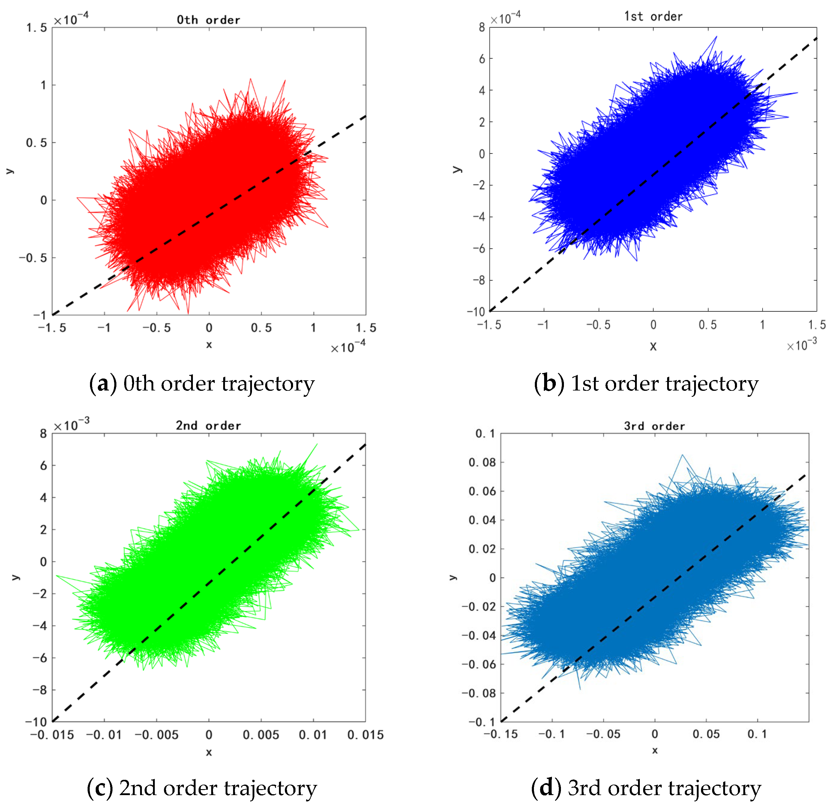
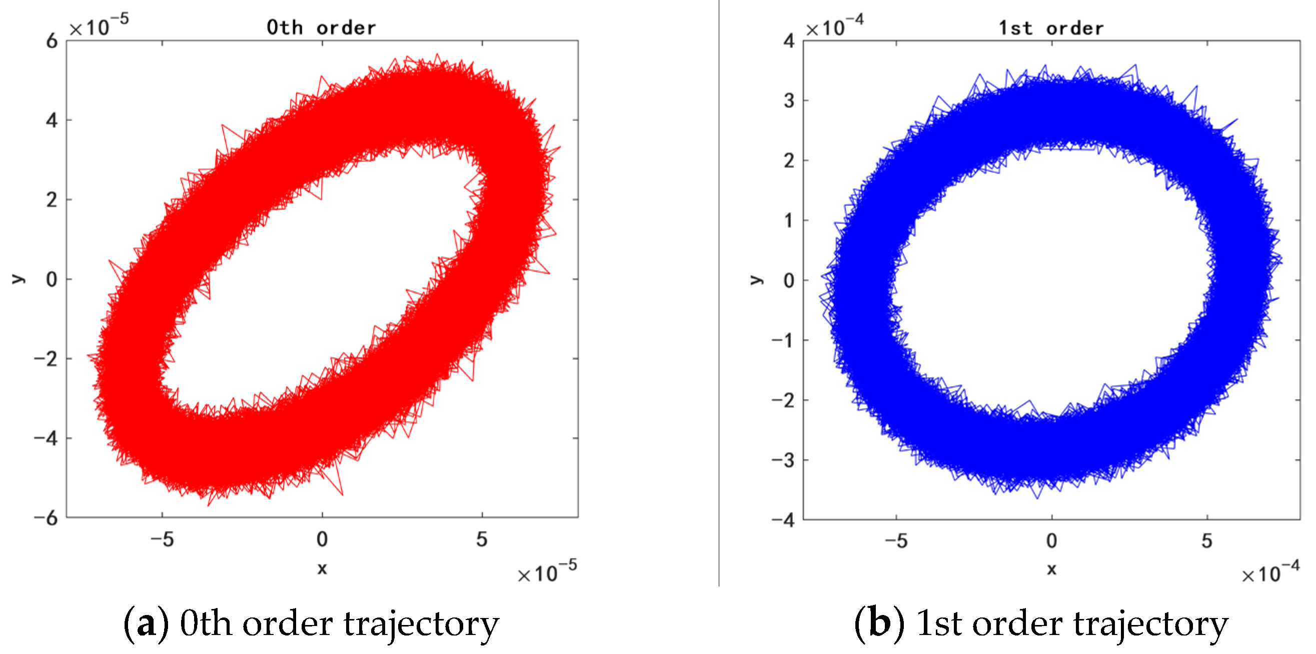
Considering that the noise influenced the particle trajectories, SNR is set as 5 dB. The different order particle trajectories of a single target are shown in Figure 3. The different order particle trajectories of two coherent signals are shown in Figure 4.

Figure 3a–d represents the 0th, 1st, 2nd, and 3rd order particle velocity gradient polarization trajectory, respectively. The black dotted line in each figure represents the straight line with the slope of tangent incident angle. We can see that the particle motion trajectory of each order is also near the theoretical line, although the noise is influenced.

Figure 4a–d represents the 0th, 1st, 2nd, 3rd order particle velocity gradient polarization trajectory of two coherent signals. The two coherent signals incident angles are 0° and 60°, respectively. It is obvious that different order particle trajectories are different.

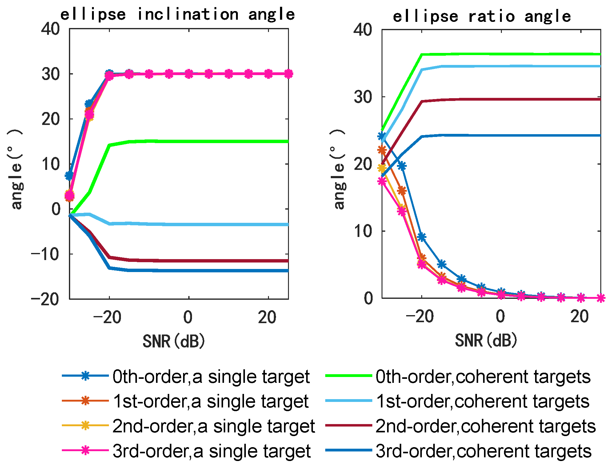
The single target incident angle is 30°, and the two coherent signals incident angles are 0° and 30°. The SNR of the received data is calibrated after the polarization filter preprocessing [31] from −30 to 25 dB at intervals of 5 dB. Here, 1000 Monte Carlo experiments are conducted to calculate the inclination angles and ratio angles of the ellipse of different order particle velocity gradients of a marine target and two coherent signals. The results are presented in Figure 5. The *lines represent the polarization characteristics of a marine target, the solid lines represent the polarization characteristics of two coherent signals, and the different colors represent the polarization characteristics of different order particle velocity gradients.

In Figure 5, when the SNR is greater than −20 dB, the inclination angle of the ellipse of different orders of a target is the same as the incidence angle. By contrast, the inclination angle of the ellipse of different orders of two coherent signals varies. The ellipse ratio angle tends toward 0° for different order particle velocity of a target, indicating a clear difference between a target and two coherent signals. From Figure 5, two coherent signals and a target can be clearly distinguished based on high-order particle velocity polarization characteristics, including the ellipse inclination and ratio angles.

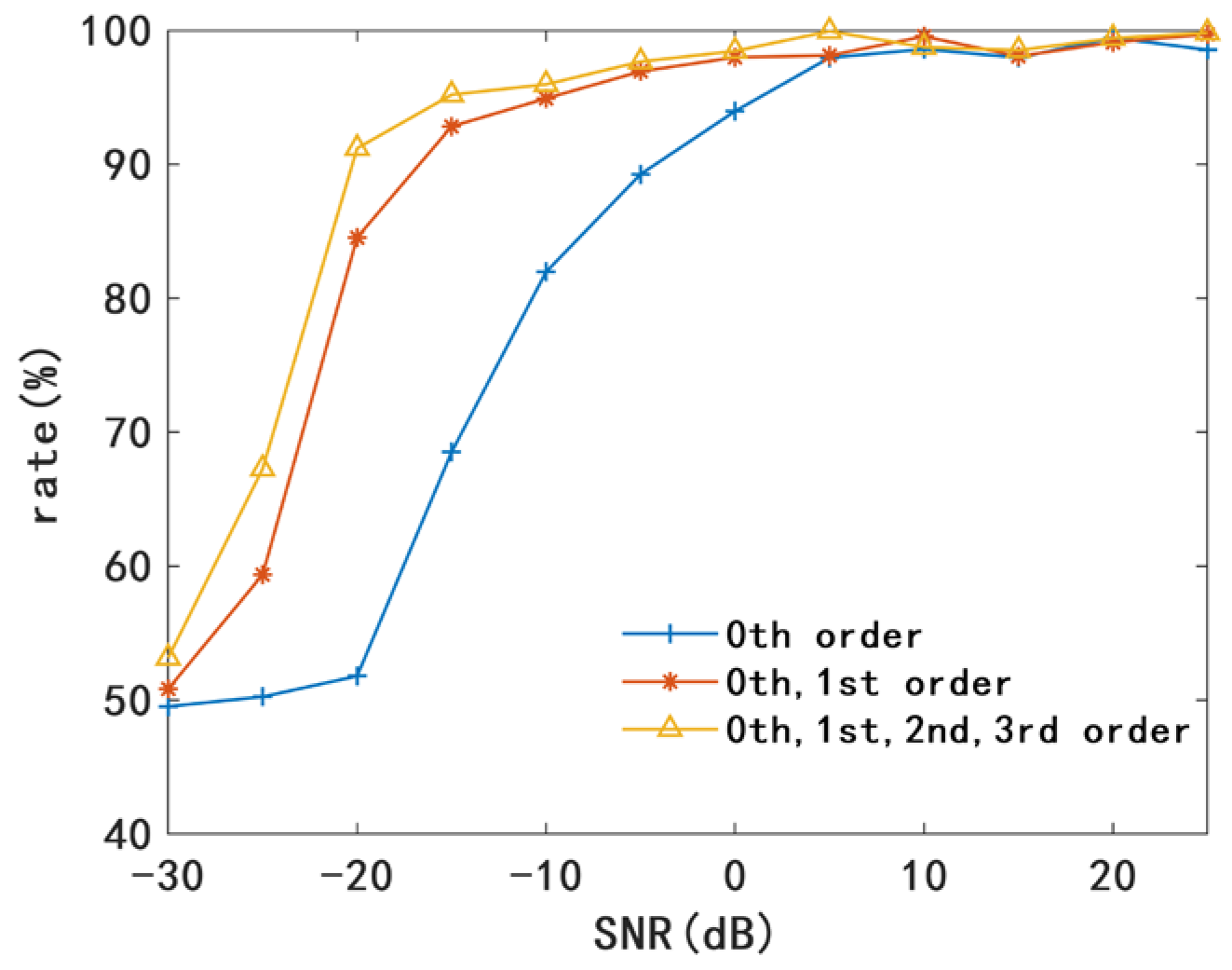
The BP neural network is used to distinguish between a target and multiple coherent signals. The polarization characteristics of a single target and two coherent signals with arbitrary angles are used as input vectors. It can be seen from Figure 6 that when the SNR is −20 dB, the particle velocity polarization characteristics are used; when the 0th- and 1st-order particle velocity polarization characteristics are used, the distinction rate is 84.54%. When the 0th-, 1st-, 2nd-, and 3rd-order particle velocity polarization characteristics are used, the distinction rate increases to 91.20%. It can be seen from the figure (0th order is + line; 0th and 1st order is * line; 0th, 1st, 2nd, and 3rd orders is ^ line) that as the order increases, the distinction rate also increases. When the SNR is greater than 5 dB, the distinction rate of the three types of polarization characteristics are all greater than 98%, and it can be verified that the high-order polarization characteristics can be used as effective features for a target and two coherent signals in water.

4. Experiment Results

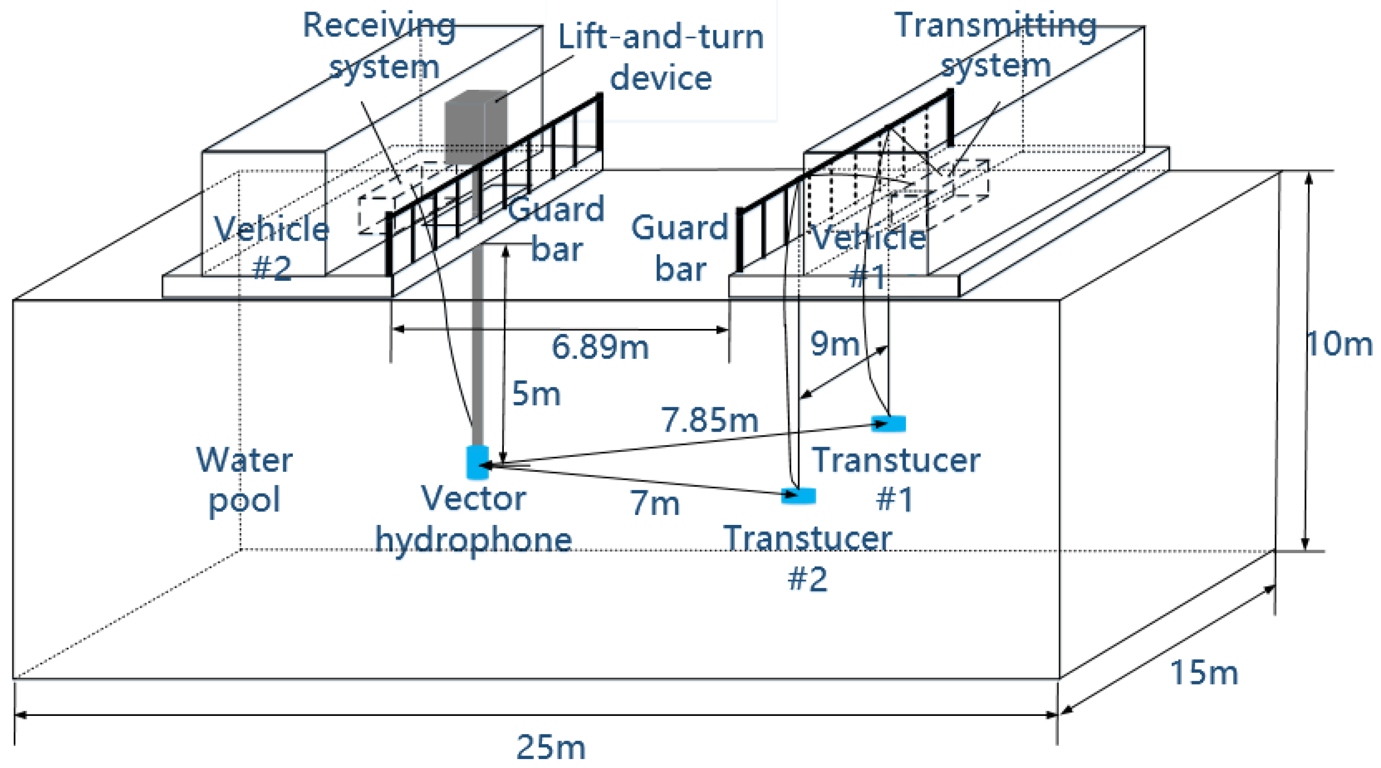
In this paper, the high-order particle velocity polarization trajectory measurement experiment is carried out in the anechoic water pool of the Acoustic Science and Technology Laboratory, Harbin Engineering University. The length, width and depth of the water pool are 25 m, 15 m and 10 m, respectively. Sound absorption wedges are laid on six sides of the pool, which guarantees the absorption coefficient above 2 kHz of the water pool is greater than 0.99. Above the lower frequency limit of 2 kHz, the free sound field conditions can be simulated. There are two mechanical moving vehicles, denoted as Vehicle #1 and Vehicle #2, above the pool for lifting equipment into the water. The schematic diagram of the experimental arrangement is shown in Figure 7. Two transducers (Transducer #1 and Transducer #2) are used to transmit signals in this experiment, which are placed 11 m apart on one side of Vehicle #1. The vector hydrophone is sealed with an oil with good transmission performance and packaged with a sound permeable shell. The vector hydrophone is placed on Vehicle #2. The distance between the two vehicles is about 3.5 m. The vector hydrophone and the sources are laid 5 m underwater.

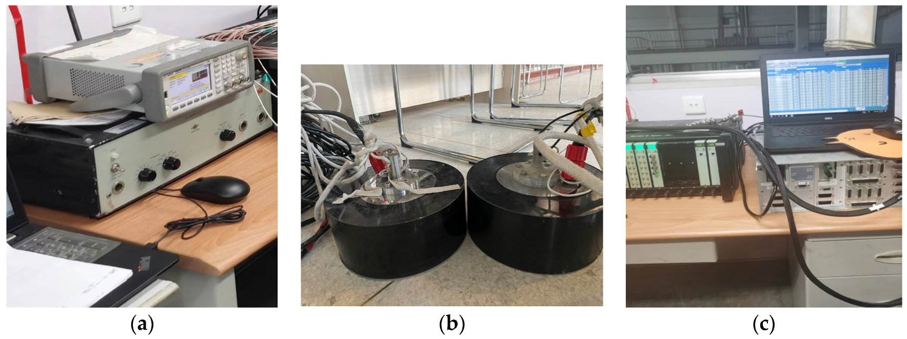
Vehicle #1 and Vehicle #2 are equipped with the experimental instrument of the transmitting system and the receiving system. Figure 8a shows the transmitting system. The transmitting system consists of two signal generators (Agilent33522A), two power amplifiers (B&K2713) and two low-frequency transducers. The cylindrical transmitting transducers are used to generate the sound signal, which is shown in Figure 8b. The diameter and the height of the transducers are about 30 cm and 10 cm, respectively. The transmitting frequency range of the transducers is from 2 kHz to 8 kHz. The receiving system is shown in Figure 8c; it is composed of a vector hydrophone, a signal conditioner (B&K2636), a data acquisition device (B&K Pulse) and a computer. Firstly, a sinusoidal signal is generated by the signal generator, which is amplified by the power amplifier and sent to the transducer. The received signals from the hydrophone are sent to the signal conditioner to be filtered and amplified, and then acquired by the signal acquisition device. The filter is set as a band-pass filter. Consider the signal frequency is 3150 Hz, the band-pass filter configuration ranges from 2 kHz to 4 kHz. Finally, measurement result processing is conducted by a computer. The signal frequency configuration of transducers in this experiment is shown in

Table 3. The signal frequency configuration of transducers in this experiment.

Cases		Case Description
1	Single-source emission	Transducer #1 transmits signals at a frequency of 3150 Hz Transducer #2 does not emit
2	Single-source emission	Transducer #1 does not emit Transducer #2 transmits signals at a frequency of 3150 Hz
3	Two-source emission	Transducer #1 transmits signals at a frequency of 3150 Hz Transducer #2 transmits signals at a frequency of 3150 Hz

.

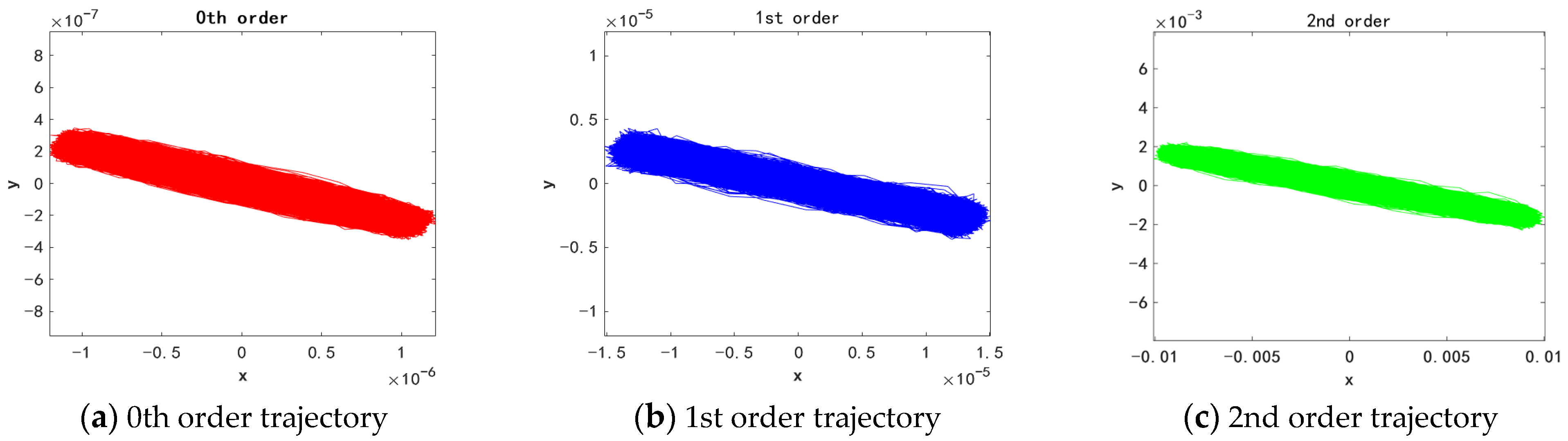
The high-order particle velocity trajectories of a single source emission are shown in Figure 9 and Figure 10, according to case 1 and case 2. They are in the same frequency but incident from different angles.

The trajectories are shown in Figure 9: (a) is the particle velocity trajectory, the ellipse ratio angle is 3.38°, and the ellipse inclination angle is 167.27°; (b) is the first-order particle velocity gradient trajectory, the ellipse ratio angle is 3.79°, the ellipse inclination angle is 168.86°; (c) is the second-order particle velocity gradient trajectory, the ellipse ratio angle is 2.56°, the ellipse inclination angle is 168.64°. 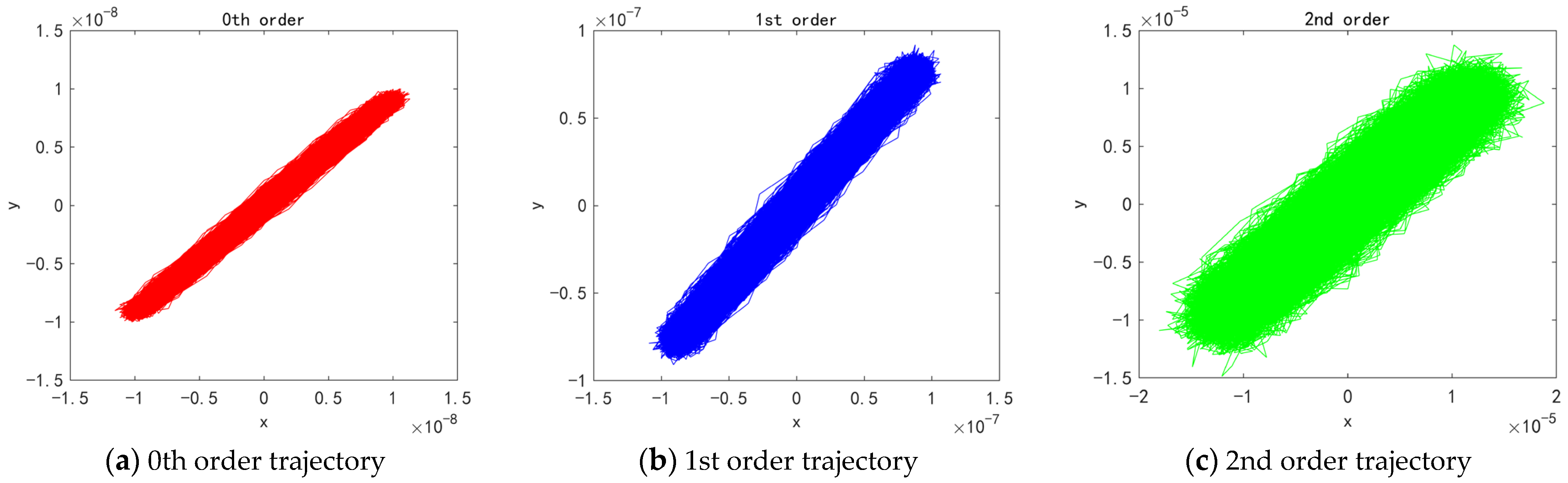Figure 10a shows the motion trajectory of the ellipse ratio angle is 2.32°, and the ellipse inclination is 47.85°. Figure 10b shows the first-order gradient trajectory of the ellipse ratio angle is 3.45°, and the ellipse inclination is 46.03°. Figure 10c shows the second-order gradient trajectory of the ellipse ratio angle is 5.28°, and the ellipse inclination is 44.60°. It can be seen from the three graphs in Figure 9 and Figure 10 that when a single target is incident, the motion traces of the 0th, 1st and 2nd orders are thick rods, and the slope is almost the same.

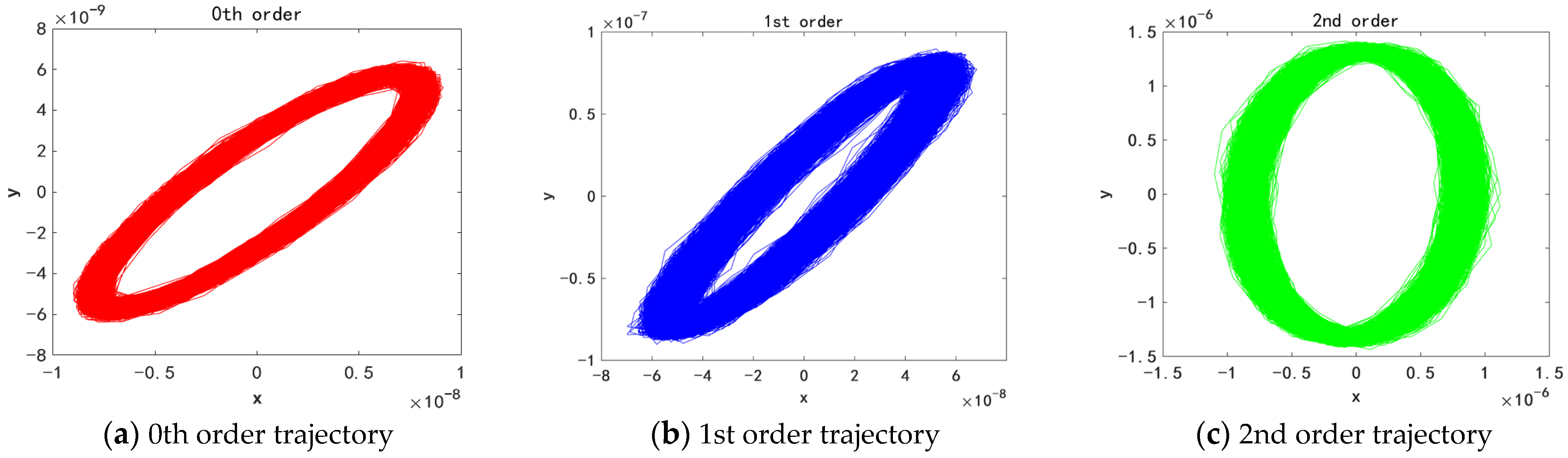
The high-order particle velocity trajectories of the two coherent signal emissions are shown in Figure 11, according to the case 3.

Case 3 is the condition of two coherent signals 1 and 2: (a) shows the particle velocity motion trajectory ellipse ratio angle is 13.99°, and the ellipse inclination is 35.43°; (b) is the first-order particle velocity gradient trajectory, the ellipse ratio angle is 10.2°, and the ellipse inclination is 56.77°; (c) is second-order particle velocity gradient trajectory, the ellipse ratio angle is 32.84°, and the ellipse inclination is 85.73°. It can be seen from the three graphs that the ellipse inclination angles and the ellipse ratio angles of the two coherent signals are different and changing; thus, we can judge whether there is coherent interference by the polarization characteristics of the high-order gradient of the particle vibration velocity.

It can be intuitively seen from the above trajectories that for a single target, the particle trajectories are thick rods, and for the coherent targets, the trajectories are ellipse. For the same single target case, the inclination angles and ratio angles of the ellipse of each order are almost the same. The average ratio angle of the ellipse of each order in Case 1 is 3.24°, and the variance is0.26°; the average inclination angle of the ellipse of each order in Case 1 is 168.26°, and the variance is0.49° The average ratio angle of the ellipse of each order in Case 2 is 3.68°, and the variance is 1.49°; the average angle of the ellipse of each order in Case 2 is 46.16°, and the variance is 1.77°. For the two coherent signals case, the average ratio angle of the ellipse of each order in Case 3 is 19.01°, and the variance is 98.03°; the average angle of the ellipse of each order in Case 3 is 59.31°, and the variance is 424.91°. It can be seen more clearly from the above statistical characteristics of each order of the particle velocity gradient polarization that the variance under the condition of a single target is small (for the experimental data, it should be less than 2°), and the variance under the condition of two coherent targets is large (for the experimental data, it should be tens of degrees or even hundreds of degrees). It can be seen that it is effective to use the high-order particle velocity polarization characteristics to judge whether the signal is a single target or two coherent targets.

5. Conclusions

In this article, the nth-order particle velocity gradient polarization characteristics of a desired target and multiple coherent signals are theoretically derived and experimentally analyzed. Different orders of particle trajectories are always a line whose slope is the tangent of the incident angle, allowing us to directly locate the desired target. In the presence of multiple coherent interferences, the trajectories of particles of different orders are different ellipses. Based on the high-order particle velocity gradient polarization properties, a BP neural network can effectively differentiate between the aforementioned two types of data following the application of a polarization filter. When the SNR is greater than −20 dB, using 0th-, 1st-, 2nd-, and 3rd-order particle velocity polarization characteristic fusion, the distinction rate is greater than 91.2%. The proposed method based on high-order particle velocity gradient polarization characteristics was verified by an anechoic pool experiment, which showed good agreement with the simulation results. In summary, the high-order particle velocity gradient polarization characteristics can be used to distinguish between the desired target and multiple coherent signals. This approach can detect multiple coherent signals with high precision on a compact platform with a low SNR and implies further practical applications in future.