TRFM-LS: Transformer-Based Deep Learning Method for Vessel Trajectory Prediction

Abstract

In the context of the rapid development of deep learning theory, predicting future motion states based on time series sequence data of ship trajectories can significantly improve the safety of the traffic environment. Considering the spatiotemporal correlation of AIS data, a trajectory time window panning and smoothing filtering method is proposed for the abnormal values existing in the trajectory data. The application of this method can effectively deal with the jump values and outliers in the trajectory data, make the trajectory smooth and continuous, and ensure the temporal order and integrity of the trajectory data. In this paper, for the features of spatiotemporal data of trajectories, the LSTM structure is integrated on the basis of the deep learning Transformer algorithm framework, abbreviated as TRFM-LS. The LSTM module can learn the temporal features of spatiotemporal data in the process of computing the target sequence, while the self-attention mechanism in Transformer can solve the drawback of applying LSTM to capture the sequence information weakly at a distance. The advantage of complementarity of the fusion model in the training process of trajectory sequences with respect to the long-range dependence of temporal and spatial features is realized. Finally, in the comparative analysis section of the error metrics, by comparing with current state-of-the-art methods, the algorithm in this paper is shown to have higher accuracy in predicting time series trajectory data. The research in this paper provides an early warning information reference for autonomous navigation and autonomous collision avoidance of ships in practice.

1. Introduction

Maritime transport is the main means of transport for economic trade and goods exchanges between countries and is characterized by high cargo-carrying capacity, low costs, and wide coverage. Up to 85% of the world’s trade is transported by sea, but the risks associated with this are greater than for other modes of transport. Ensuring the safest possible navigation of transport vessels at sea is the most basic requirement for maritime transport. In particular, when ships are navigating in and out of a channel, the density of passing ships in the limited space is greater than in the outer sea, and even with the aid of pilots, merchant ships still have a high navigational risk when entering and leaving the channel. It is therefore essential to predict the trajectory of ships reasonably navigating in the channel. The forecast can largely reduce navigational risk and ensure safe navigation.

Today, the marine industry is also undergoing a technological revolution known as the Ship 4.0 era [1]. More and more sensors for data collection are being used in the waterway transport system [2], among which the Automatic Identification System (AIS) is an important data resource in the maritime transport system. The AIS can automatically and regularly broadcast dynamic information such as real-time ship position, heading, speed, and track direction as well as static information such as ship name, call sign, ship type, and ship scale via very high frequency (VHF). These data are automatically received by ships or base stations with AIS equipment within the VHF coverage area (approximately 20 nautical miles). Further developments in real-time communications at sea and shipborne data transmission [3] provide favorable data conditions and information for researchers to obtain large amounts of vessel trajectory data and to explore further ship movement characteristics. Ref. [4] combines the concept of TCR and a large AIS data source in a large-scale and real-time maritime traffic environment to identify the ships with potential for collision accidents.

Trajectory prediction of objects utilizes the historical trajectories and behaviors to forecast their future motion, which to a certain extent can significantly improve the safety of the traffic environment. Inspired by the Transformer algorithm model in deep learning, we implement a method for predicting temporal sequence data, TRFM-LS, by architecting the LSTM module in the decoder output layer. Transformer can be thought of as a deep learning model based entirely on attentional mechanisms. The LSTM has the ability to convey spatiotemporal properties of sequential data, while the complex internal structure of the Transformer provides a powerful parallel computing capability. This combination of LSTM and Transformer complements the weakness of the LSTM-based model prediction algorithm in capturing information when predicting from a distance. Comparative experiments also demonstrate that this paper’s method outperforms prediction methods that rely entirely on recurrent neural networks in terms of performance and accuracy.

1.1. Related Work

Trajectory prediction has been widely studied in many fields [5], including vehicle trajectory prediction, pedestrian trajectory prediction, and robot trajectory prediction.

Similarly, many scholars have conducted in-depth research on ship trajectory prediction, which has evolved from traditional statistics-based prediction to machine learning-based prediction and nowadays the popular deep learning-based prediction. There is also a large body of literature on the application of historical AIS data combined with algorithmic models for predicting ship trajectories. For example, in [6], a waypoint estimation algorithm was presented to estimate the waypoints of the interpolated representative trajectory. Ref. [7] considered the problem of prediction accuracy in constrained waterways and used real-time estimation of system noise in the Kalman filter algorithm to predict ship trajectories in the state of insufficient AIS information of ships. Ref. [8] constructed a BP network structure to predict the future trajectory of a ship by inputting historical trajectories and current information from AIS data. Ref. [9] predicted traffic trajectories based on Bayesian probability by introducing a bi-directional long short term memory mixed-density network (BLSTM-MDN). Ref. [10] proposed a new bi-linear autoencoder method that uses clustering of historical AIS trajectories to iteratively predict the entire trajectory of future states, and the predictions rely on the effectiveness of the previous clustering.

With the development of deep neural networks, the long short-term memory (LSTM) network has become the primary method for trajectory prediction. LSTM sequentially processes time series data to characterize the position, direction, and speed of agents [11]. As a kind of time series data, the LSTM algorithm is also applicable to the time series prediction of ship trajectories. The LSTM algorithm not only produces good predictions when applied alone [12], but its deformed method also has good prediction performance, e.g., Ref. [13] predicts the trajectory sequence of a ship including longitude, latitude, speed, and heading characteristics for the next 5–20 min using a variational LSTM. GRU is similar to LSTM as both are variants of the RNN and, in [14] a ship trajectory prediction model is developed based on the combination of a multi-headed attention mechanism and GRU.

At the same time, the combination of LSTM and other algorithms has been successfully applied in the study of trajectory sequence prediction. Many scholars have combined LSTM models with other models as a new method for prediction, and these combined models have certain feasibility and effectiveness, e.g., Ref. [15] combined the extended convolutional network and LSTM algorithm to form the time series model DC-LSTM, and applied the extended convolutional network to extract the features of the predictor variables, and then input them into the LSTM together with the historical data to obtain the desired multi-part prediction effect. Ref. [16] combined the LSTM algorithm with the TPNet algorithm to achieve a balance between the accuracy and complexity of trajectory prediction. Ref. [17] fused LSTM into an encoder–decoder framework and formed a recurrent neural network to predict sequence-to-sequence ship trajectories, which showed that sequence-to-sequence neural network-based deep learning trajectory prediction outperformed linear regression or feedforward networks.

In summary, most of the predictions of trajectories by LSTM algorithms are driven by big data to learn the behavioral features of agents, which is common to almost all recurrent networks. LSTMs can implicitly model the inherent dependency between the consecutive observations of ships’ trajectories in an end-to-end fashion. Despite all this, LSTMs were recently argued to be inefficient when it comes to modeling longer sequential data [18]. In addition, LSTMs were also shown to be more sensitive to missing observations which is typically the case with any data coming from real physical sensors [19].

As deep learning is increasingly researched within various specialized fields, recurrent networks (e.g., LSTM) show some weaknesses in big data prediction. Transformer networks [20] were recently introduced and quickly became the preferred model when it comes to sequential modeling tasks such as natural language translation and generalization [21]. In [22], since the study of natural language processing does not involve temporal properties, only one layer of LSTM is attached to the front end of masked multi-head attention (MHA) in Transformer, which provides a complementary historical representation for attention-based representations.

The Transformer algorithm discards the traditional CNN and RNN, and the structure mainly consists of a self-attention and feedforward neural network. Its advantage is that it enables parallelized computation, and its prediction performance has achieved good results within the field of natural language processing, and also promotes the possibility of using Transformer for temporal data prediction in other fields. Ref. [23] constructs the Transformer-XL model based on Transformer, which makes it possible to learn independently beyond a fixed length. Ref. [24] constructed a Longformer model based on Transformer, which predicts longer time series data series. Ref. [25] constructed the Traffic Transformer model based on Transformer, which captures the continuity and periodicity of time series according to the model. It is not difficult to find that, in time series prediction, many prediction studies incorporate an attention mechanism into the algorithm [26,27], which makes the model pay more attention to the features of data dimensions in predicting time series data and the learning of the model is more purposeful and the output of the predicted result is more in line with the real desired state. For example, Ref. [19] used Transformer for the motion trajectory prediction of pedestrians. Compared with the LSTM model, which processes sequential data in a step-by-step sequence, the Transformer model learns sequential data features mainly based on the attentional memory mechanism and achieves trajectory prediction of independent individuals’ actions in real scenes.

1.2. Contribution

1. A time window panning and smoothing filtering method is proposed. A fixed-step time window is constructed based on the time interval of AIS trajectory data, and the data within the time window are smoothed and filtered. The time window is panned along the time axis on the trajectory so that the data distribution of each vessel history trajectory tends to be homogenous and smooth. Such an operation not only corrects the trajectory points that deviate from the actual movement pattern but also revises the wrong points in the trajectory, further ensuring the global validity of the data.

2. Some deficiencies are improved when using LSTM to predict trajectories. In the process of learning trajectory sequence data by LSTM, the hidden layer can only generate and pass the intermediate information of fixed length to the input sequence and cannot distinguish the importance of feature information of the sequence, which makes the operation long and unfavorable to the improvement of prediction accuracy. In this paper, we apply the multi-headed attention mechanism in Transformer to focus on the weight of feature information in the trajectory sequence and give more weight to the key information in the input vector, to predict more accurate results and effectively improve the prediction accuracy.

3. The structure of the Transformer model for sequence data prediction is improved. The complementary nature of LSTM is added by combining the LSTM module with the Transformer prediction framework. The LSTM module can learn the temporal characteristics of the data in the process of computing the target sequence, and the self-attention mechanism in Transformer solves the shortcoming of LSTM in capturing weak information of the sequence at a distance.

The remainder of this paper is organized as follows: Section 2 focuses on the spatiotemporal pattern mining of vessel trajectory data and a new filtering method for trajectory data. The third section is the main research method of this paper, the fourth section is the experimental comparison analysis, and the fifth section is the conclusion.

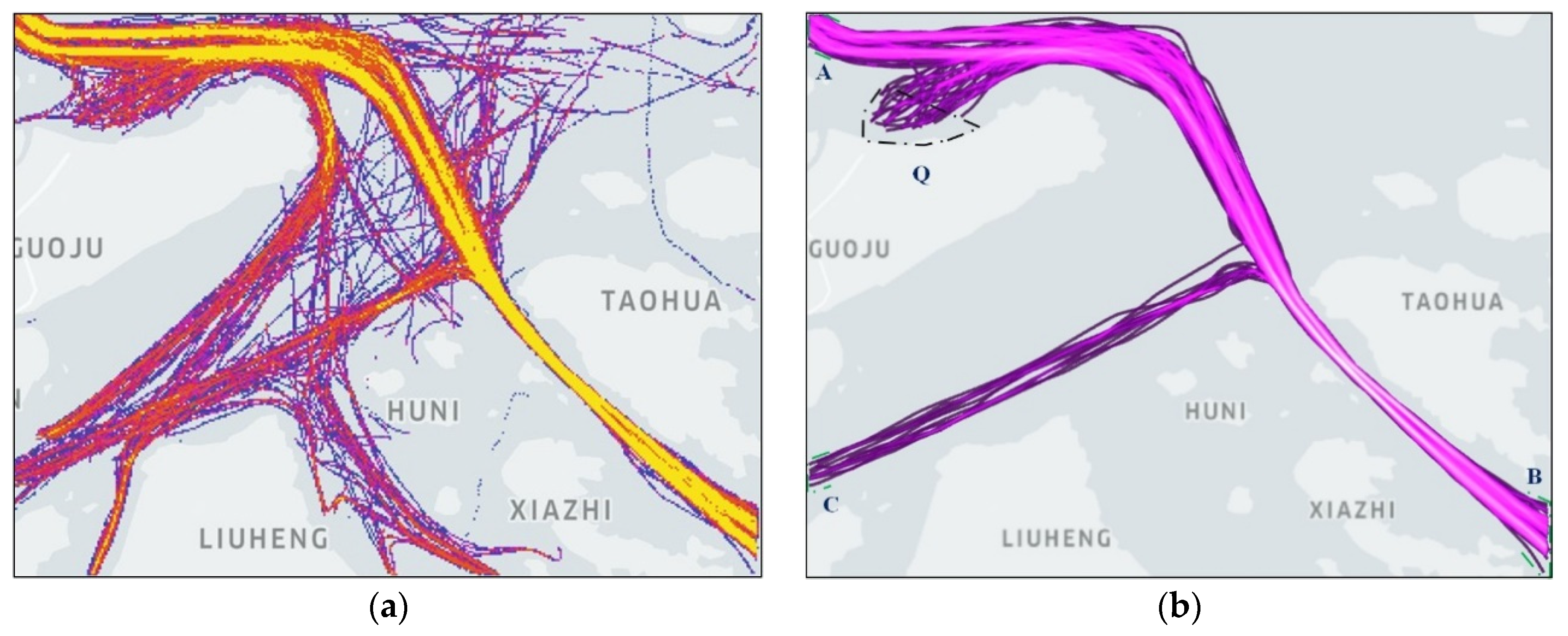
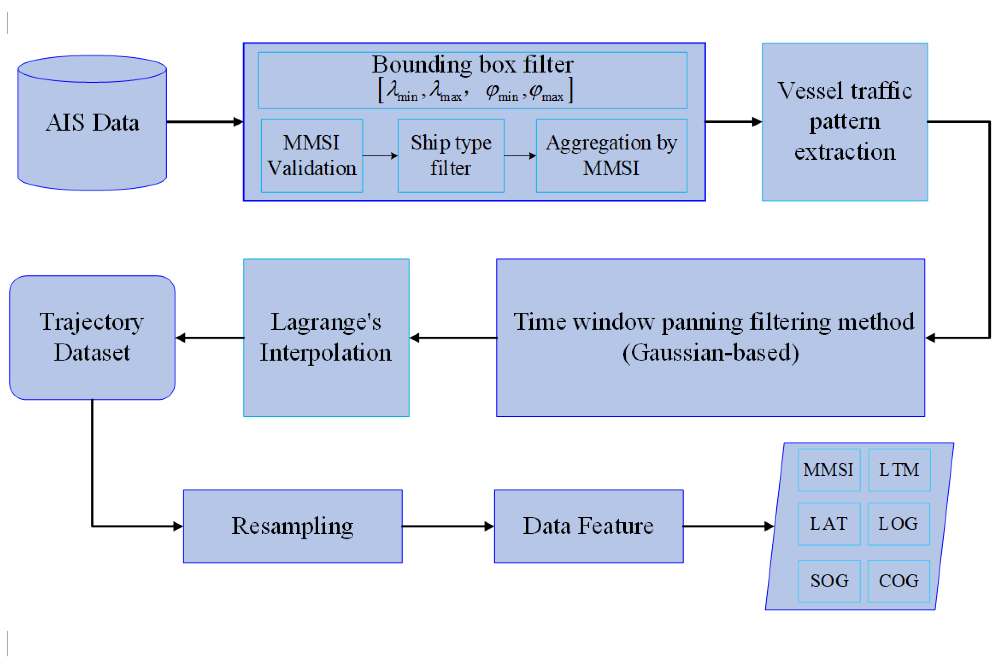
2. Vessel Traffic Spatiotemporal Pattern Extraction and Data Processing

In the process of ship trajectory prediction, data processing and deep learning model construction are the two keys to ensure the accuracy of ship trajectory prediction. The aim of ship trajectory prediction is to predict the ship’s navigation dynamics in the future period by establishing an accurate prediction model framework based on the multi-dimensional characteristics of the ship’s historical trajectory big data. As a source of information that reflects the real-time dynamics of a ship and its historical state and can be effectively stored, AIS becomes the main information for predicting the spatiotemporal relationship of a ship in the future period.

AIS plays an important role in identifying ships, tracking targets, and revealing the state of maritime traffic. AIS data are multi-dimensional spatiotemporal data, which contain a wealth of spatiotemporal information and correlations between the various attributes. AIS information can reflect the busy state of maritime traffic and the pattern of connection between different routes and ports. The most intuitive tool to reflect the state of maritime traffic is the density map of traffic distribution as shown in Figure 1a, which shows the density map of vessel AIS trajectory data distribution in Ningbo-Zhoushan waters off the coast of China. From Figure 1a it can be seen that although there is a high density of ship traffic in the water, the ships are not randomly distributed. There is a potentially regular distribution of routes within the ship traffic flow, but the difference is that the density varies with the location of the route and indirectly reflects how busy the route is. In the historical data of traffic flows, when the starting and ending locations of the traffic flows are defined, the AIS of the spatial distribution of traffic flows between two regions such as (A, B), (B, C) or between a region and a port such as (Q, B) can be selected, as shown in Figure 1b. Section 4 describes how these data were used as training for the deep learning models in this paper.

However, the transmission of AIS data is based on time division multiple access technology and the data are inevitably subject to signal interference during transmission. In addition, human factors such as possible mishandling of the equipment make it difficult to use the AIS data directly for model training and research. We need to preprocess the data according to the mechanism of the model and the needs of the research objectives. This paper proposes a smoothing and filtering method for the problems that appear in the actual state of the ship’s AIS trajectory, which can make the AIS data more learnable in line with the model.

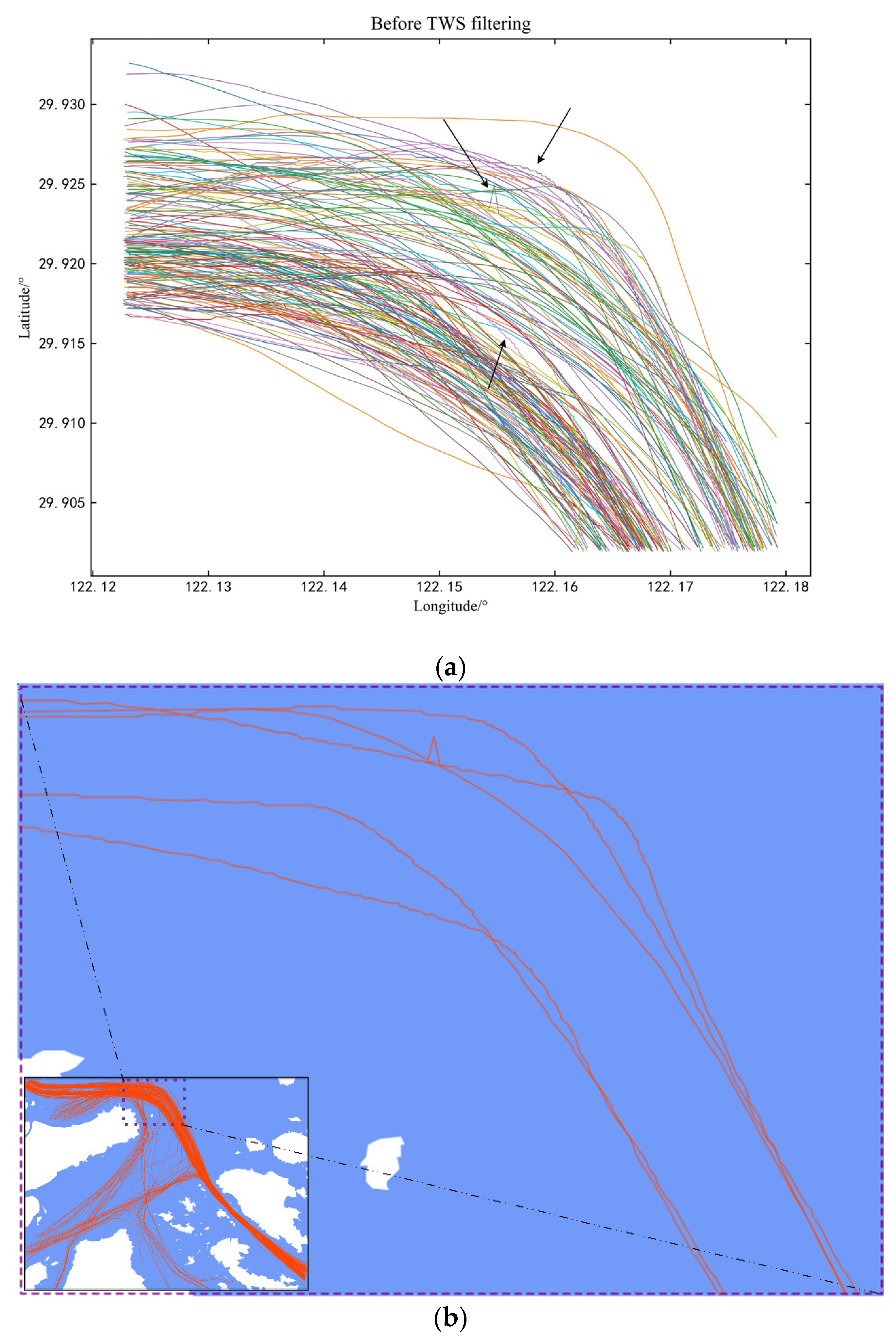
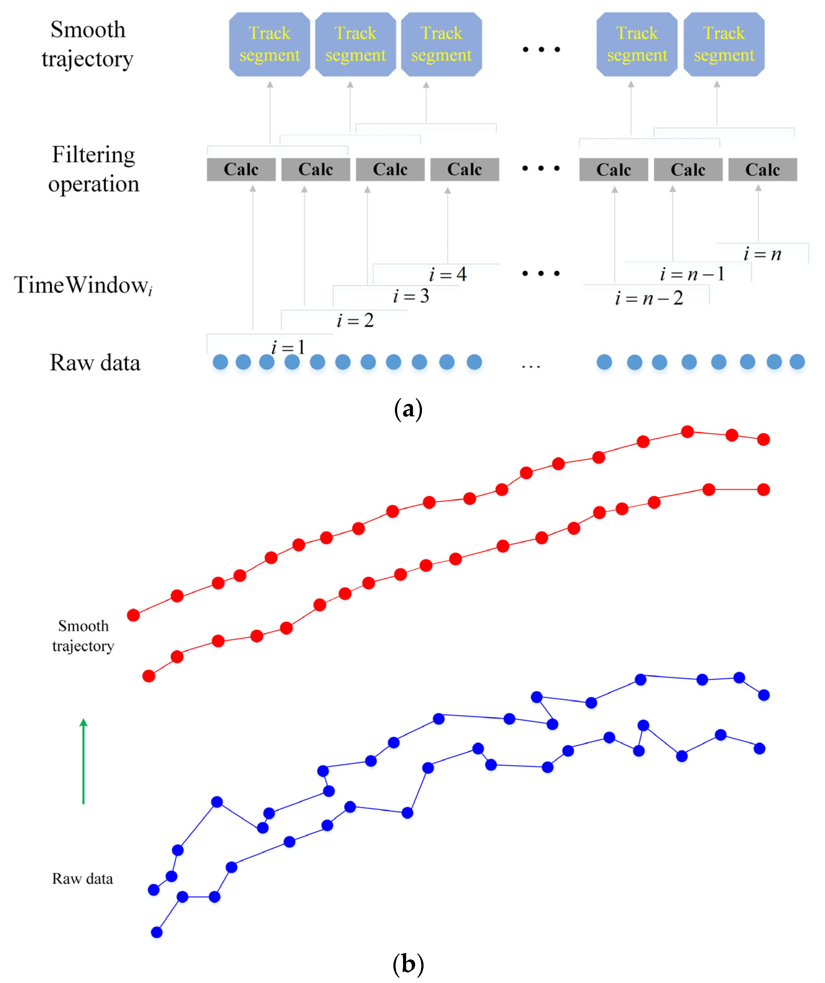
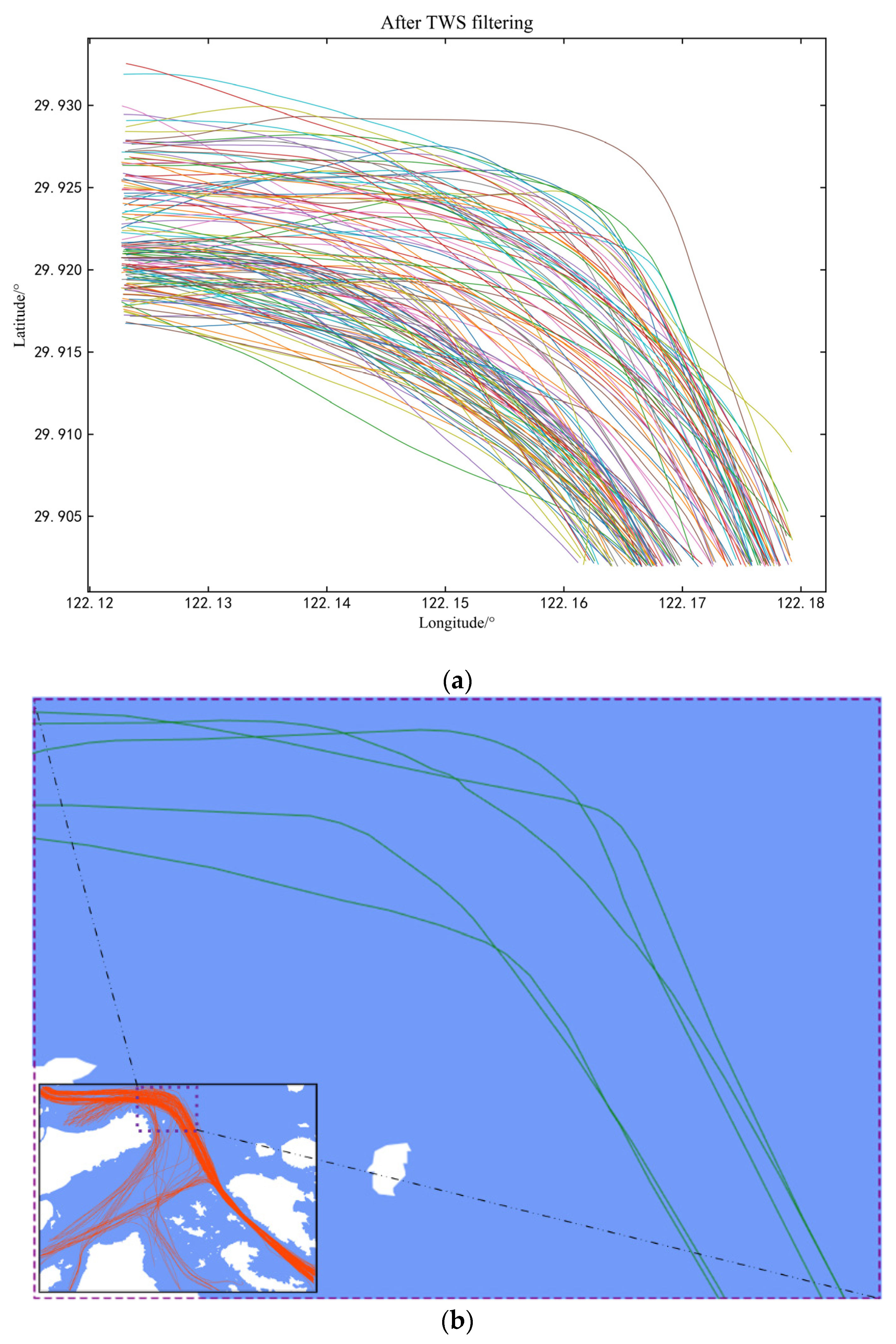
2.1. A Time Window Panning Filtering Method for Trajectories

Since there is a certain time gap between the original ship’s historical trajectory data being transmitted and received, the corresponding spatial distribution of the trajectory data in the state of a continuous time series does not match with the actual movement of the ship. As a result, many data in the ship trajectory appear locally jagged or rippled. Figure 2a shows the ship trajectory after selecting the geographic box, and it can be seen that many trajectories have localized jagged or ripple-like anomalies. In order to show the anomalous part of the original data more clearly and visually, we zoomed in on the local part of some anomalous traces in Figure 2a and mapped several tracks as shown in Figure 2b. The above data with anomalous trajectories neither conform to the real hydrodynamic motion of the ship nor contribute to the learning of data features by the algorithm model, which leads to large errors in predicting the spatial and temporal information of the trajectory.

For the problems of the above trajectories, this paper proposes a filtering method called “time window panning smoothing filtering”. The duplicate data and outlier data in the database need to be removed before filtering. We build a dataset $D=\left\{X^k,\left(k=1,2\cdots ,N\right)|X\in \Theta \right\}$ of trajectory sequences based on MMSI identification numbers, where $\Theta$ denotes the range of geographical areas in which the ship trajectories are located, while $X^k$ denotes the trajectory sequences of ships with different MMSI. For any trajectory, a segment can be represented by $X^k=\left\{{\tau }_i^k;i=1,\cdots ,{\rm T}\right\}$, where ${\tau }_i^k$ denotes the temporal and spatial information of the trajectory point, ${\tau }_i^k$ has the temporal and spatial properties of the trajectory point, $\tau =\left\{\left(t_j,x_j,y_j,v_j,c_j\right)\right\}\left(j=1,2\cdots ,n\right)$ denote the longitude, latitude, speed, and heading at the time of $t_j$, respectively.

The main feature of time series data is that it is possible to describe changes in the state in the historical time dimension of the object based on its time dimension. Ship trajectory data are typical of time series data, where the position, speed, and heading of the ship need to be indexed by the time dimension. Therefore, filtering operations on trajectories need to be modeled with the time dimension as a reference. During the filtering and smoothing operation of the trajectory, the time within the time window is selected as the reference point, so that the time reference is sequential moment points within the window in order. The kernel function is constructed by calculating the difference between the time in the window and the time reference point, and the kernel function performs the dot product operation with the trajectory features corresponding to the traversed time, as shown in Figure 3a. After that, the filtering of all trajectory feature data is completed by panning the time window and, finally, the smoothing filtering operation of the whole trajectory segment is gradually realized. The mechanism of the smoothing filtering operation is shown in Figure 3b. When determining the size of the time window, taking into account the frequency of AIS launch and the sampling interval of the training data required by the model in this paper, the time window size is set to 60 s. When filtering and smoothing successive adjacent trajectory points, they are based on a Gaussian kernel function for the trajectory feature data within the window, as in Equation (1).

$$𝒲(t)=\frac{1}{\sqrt{2\pi }\mathsf{\Delta }{t}_w}{e}^{-{\displaystyle \frac{t_{p_i}-t_r}{2\mathsf{\Delta }{t}_w}}}$$

(1)

where $\mathsf{\Delta }{t}_w$ denotes the size of the time window, $t_{p_i}$ denotes the moment of the $i$th point in the window, $t_r$ denotes the base reference time within this window.

Compared with the original trajectory before filtering, the rippled or jagged trajectory points are removed from the ship trajectory data after the above time window panning filtering algorithm. At the same time, the points in the trajectory that deviate from the actual motion position of the ship are corrected. The trajectory data are shown in Figure 2a and Figure 4a. Both come from the same selected geographic box and those in Figure 4a are displayed as the trajectory in Figure 2a after the smoothing and filtering operation. It can be seen that any AIS trajectory in the figure is continuously smooth and homogeneously distributed after the filtering operation. Similarly, the trajectory in Figure 4b is the mapping of the anomalous trajectory in Figure 2b after the filtering process.

2.2. Other Preprocessing of Trajectory Data

As mentioned in the previous smoothing filtering research, anomalies in the trajectory need to be removed before smoothing. Anomalies mainly include duplicate values, error values, and outliers. Duplicate values refer to the values where the time indexes overlap and the values of each field are continuously the same in the trajectory generated by the navigation process. An error value means that the longitude and latitude information of the track point is beyond the selected waters or the values of COG, SOG, HED, etc. are beyond a reasonable range. Outliers refer to jump values with large deviations between voyages with small distances, usually due to incorrectly recorded information for a single point. These anomalies will affect the subsequent data analysis and application of the model, which in turn affect the prediction accuracy of the algorithm, so such anomalies should be processed. Duplicate values can be handled by retaining one of the values and deleting the rest of the same values, and error values and outliers also need to be interpolated to fill in the vacant bits after deletion.

The complete AIS trajectory is composed of a continuous sequence of points during the ship’s voyage, and it is more appropriate to apply the interpolation method for the complementary processing of the vacant values. For the characteristics of the small time interval of the trajectory sequence, the application of the cubic spline interpolation method has some advantages in the smoothing of the trajectory. Therefore, the method of cubic spline interpolation is used in this study. The functional equation of cubic spline interpolation is shown in (2). Assuming that the period time of the sequence to be interpolated is divided into $n$ intervals $\left[\left(x_0,x_1\right),\left(x_1,x_2\right),\cdots ,\left(x_{n-1},x_n\right)\right]$ and if $n+1$ points $y_0,y_1,\cdots ,y_n$ satisfy the function Equation (2), then the data can be interpolated at equal intervals according to the conditions satisfied by the cubic spline equation and the adjacent data points.

$$S_i(x)=a_i+b_{i}x+c_i{x}^2+d_i{x}^3$$

(2)

where $a_i$ $b_i$ $c_i$ $d_i$ are the coefficients to be determined. The time interval of the AIS data selected for the experiments in this paper is mostly the emission frequency interval, which is generally 2–10 s. The intensive time interval cannot test the prediction accuracy of the model and the information of the predicted future moments will also lose its practical significance. Therefore, it is necessary to resample the above preprocessed data according to the research of this paper. In this paper, the time interval of resampling is 1 min, and the future time period of prediction can be determined according to the length of the sequence predicted by the model.

In order to make the prediction network converge quickly and avoid the impact of data on training due to different magnitudes and quantiles, the data are normalized here. In view of the fact that the numerical distribution of the experimental data has no obvious boundaries, this paper adopts the mean variance normalization method to normalize the data, and the equation of mean variance normalization is shown in (3).

$${\tilde{S}}^j=norm(S^j)=\frac{S^j-S_{mean}^j}{S_{\max }^j-S_{\min }^j}$$

(3)

where ${\tilde{S}}^j$ is the normalized value, $S_{mean}^j$ is the mean value, $S^j$ is the original data, $S_{\min }^j$ and $S_{\max }^j$ are the minimum and maximum values of the original data, respectively.

The process of the above data processing is summarized in Figure 5.

3. Methodology

In this part of the study, a deep prediction model method based on historical ship trajectory data is mainly established, and the method is used to predict the ship’s trajectory in the future period.

In order to improve the prediction accuracy and better adapt to the learning of spatiotemporal sequence type data, this paper combines the advantages of Transformer and LSTM to propose a trajectory prediction method incorporating an attention mechanism, which is named TRFM-LS prediction in this paper.

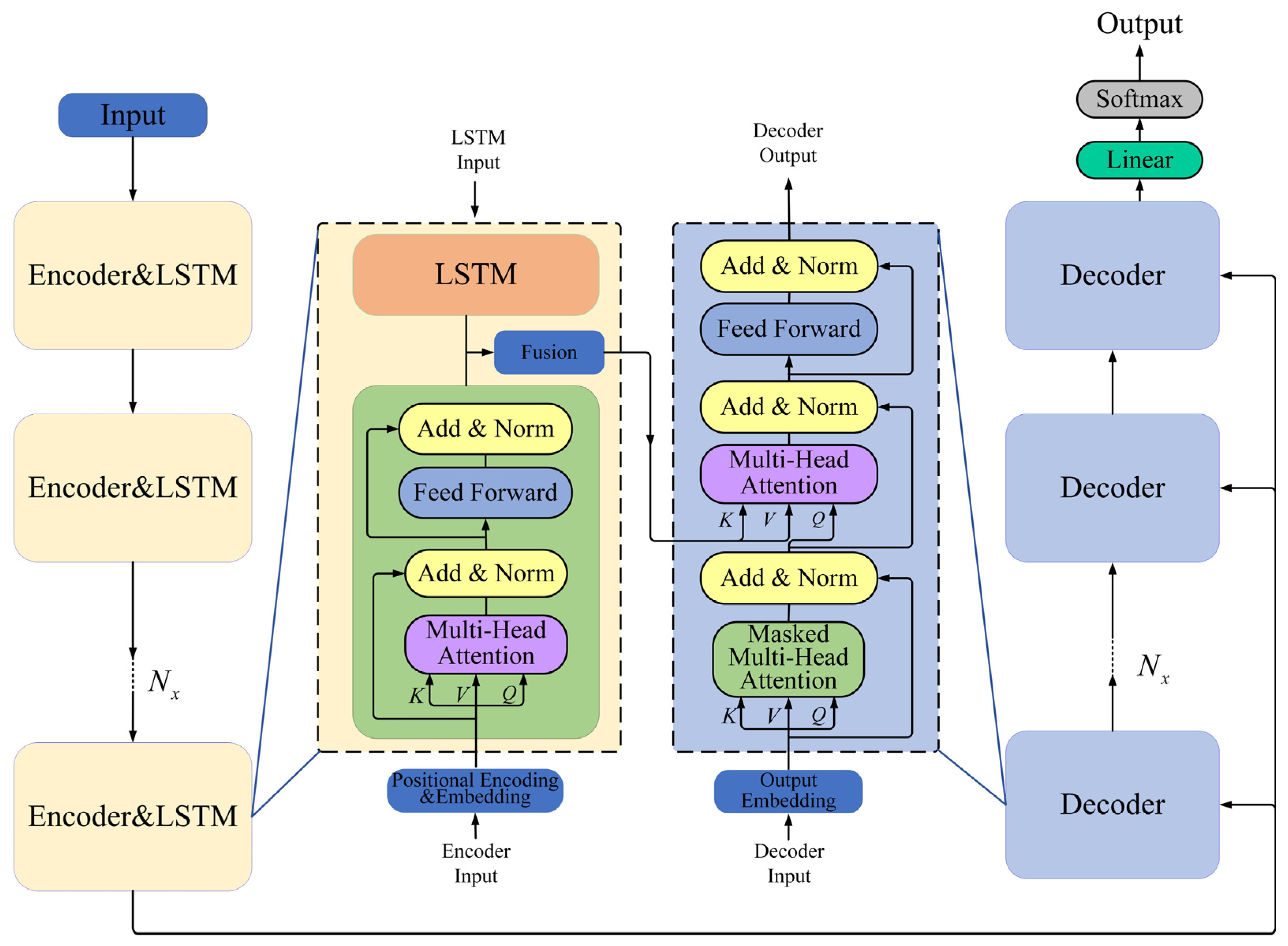
3.1. Transformer Model Main Architecture

Transformer is a deep learning model that utilizes encoder and decoder structures for sequence modeling [20]. Transformer networks no longer rely on the structure of time series in RNN-based neural networks. Transformer also differs from the seq2seq model which only captures the relationship between the input source and the predicted target while ignoring the respective internal relationships. As shown in Figure 6, the main network structure of the Transformer model framework consists of two parts, the encoder block and the decoder block. The framework mainly relies on the self-attention mechanism and sub-modules of multi-headed attention for nonlinear learning of time series data and spatial data internally.

As a new type of model that is capable of handling sequential data, the Transformer sub-module also gives the model the ability to train data in parallel. Thus, when an AIS trajectory containing multi-dimensional features is embedded in the Transformer architecture in a certain batch, the model is based on temporal and spatial information delivered to the multi-headed attention mechanism and stacking layers in the architecture to be able to learn dynamic and hierarchical features in the sequence data. It is also the difference between Transformer and recurrent neural networks in predicting sequence data.

3.1.1. Positional Encoding

As shown in Figure 6, the framework has mainly feedforward structures instead of the previous main convolutional or recurrent structures. Thus, the Transformer module processes the sequential structure of the trajectory sequence differently from the recurrent neural network, which mainly relies on self-attention to encode the temporal and spatial attributes of the trajectory sequence. The encoding ${ℰ}_{obj}^{\left(i,t\right)}$ embedded in the input sequence contains the embedding of the temporal position encoding ${𝒸}_{obj}^{\left(i,t\right)}$ and the spatial position encoding ${𝒫}^t$ vector of the trajectory sequence. Referring to the setting in [20], this paper uses the $\sin$ function and $\cos$ function to encode the location information as in the following Equation (6).

$${ℰ}_{obj}^{\left(i,t\right)}={𝒸}_{obj}^{\left(i,t\right)}+{𝒫}^t$$

(4)

$${𝒫}^t={\left\{𝓅\left(t_{pos},d\right)\right\}}_{d=1}^D$$

(5)

$$\{\begin{array}{l}𝓅\left(t_{pos},2d\right)=\sin (t_{pos}/{10000}^{2d/D})\\ 𝓅\left(t_{pos},2d+1\right)=\cos (t_{pos}/{10000}^{2d+1/D})\end{array}$$

(6)

where $t_{pos}$ represents the time position of the input vector in the input sequence, $d$ denotes the vector dimension.

Positional encoding is very important for the model, because each dimension of the positional encoding varies in time according to a sinusoid of different frequency. This ensures a unique time stamp for sequences of up to 10,000 elements and extends unseen lengths of sequences. At this point, Transformer differs greatly from the RNN. The RNN processes the input sequentially and the order of input positions determines the flow of time. It needs to “unroll” at training time, i.e., back-propagate the signal sequentially across the cell or blocks processing the observations. By contrast, the training of Transformer is parallelizable. Notably, thanks to the positional encoding which time stamps the input, Transformer may deal with missing observations. Missing data are just neglected, but the model is aware of the relative time stamps of the presented observations.

3.1.2. Encoder–Decoder Transformer

Encoder–decoder is an essential structural component of the Transformer, its key content is the internal attention mechanism. The processed historical ship trajectory positions are fed to the network, and the network predicts the future trajectory. In this work, the encoder–decoder network is composed of six encoder blocks and six decoder blocks. Every encoder block has two sub-layers, a multi-head attention layer, and a feedforward network layer. The multi-head attention layer uses self-attention to learn the relationships of the input sequences. The other feedforward layer is a fully connected network responsible for the linear transformation and ReLU activation function for each position vector. The output of the encoder block is passed on to the next encoder block or decoder. All encoding processes are parallel, which greatly improves the efficiency compared to the model in the original RNN.

Similar to the encoder block, each decoder block consists of three sub-layers, two multi-head attention layers, and a feedforward network layer. The first part of the attention layer uses self-attention to learn the relationships within the target sequence. The output of this layer is fed into the second attention layer together with the results passed from the previous encoder. The latter is not a self-attention layer, but encoder–decoder attention, which is mainly used to learn the relationship between the input sequence and the target sequence. To prevent degradation and accelerate convergence, residuals and layer normalization are added behind each layer in the encoder block and decoder block.

3.2. TRFM-LS Trajectory Prediction Model

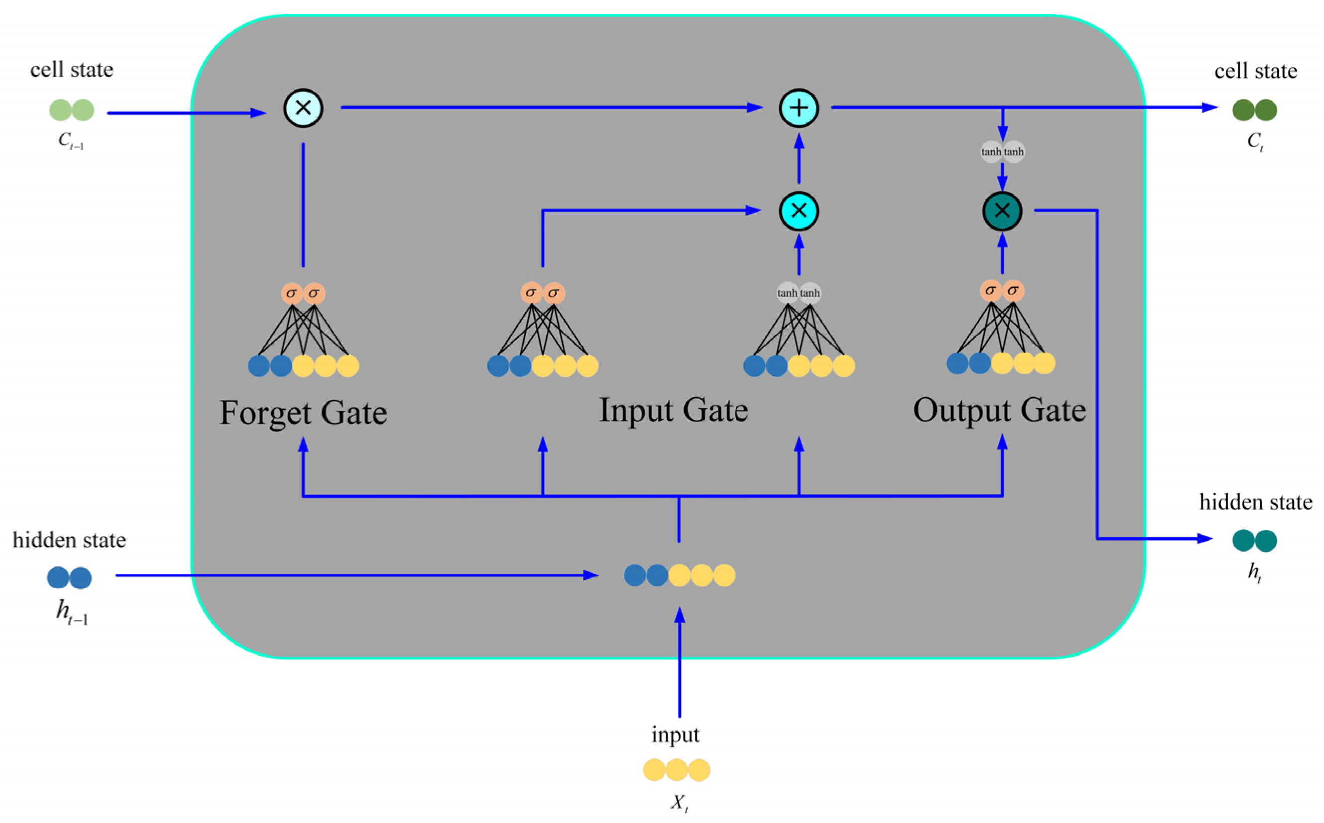
3.2.1. Transformer–LSTM Fusion Structure

In this section, to exploit the complementarity of the long-term representation of LSTM hidden states, the TRFM-LS trajectory prediction structure is proposed and an LSTM model is added to the Transformer block as shown in Figure 6.

After position encoding, the sequence is sent to the encoding module of the Transformer, while the sequence is also sent to the LSTM module for processing. LSTM is a special structure of the RNN, which solves the problem of gradient disappearance and explosion when dealing with longer time sequences. The core part of the LSTM network is the hidden layer memory block with stored states. This hidden layer block contains three gate structures, which are the forget gate, input gate, and output gate. The structure in the memory block of the hidden layer is initialized by the final hidden state of the past segment (n − 1), as shown in Figure 7. This hidden layer block allows the sequence data to pass through the entire cell without information loss, and only a small number of linear operations are performed to achieve memory retention of the spatiotemporal data characteristics of long time series.

The sequences which are input to the LSTM module are processed by a separate LSTM. The reason for choosing LSTM is that it can be considered a decomposition process. As this study is a time series modeling problem, temporal features are important in corresponding to spatial features. We use LSTM to accomplish the embedding of temporal features. Thus, these models extract temporal and spatial features step by step.

$$\{\begin{array}{l}{f}_t=\sigma (W_t\cdot [h_{t-1},x_i]+b_f)\\ i_t=\sigma (W_i\cdot [h_{t-1},x_t])\\ {\tilde{C}}_t=\tanh (W_c\cdot [h_{t-1},x_t+b_c])\\ C_t=f_t\cdot C_{t-1}+i_t\cdot {\tilde{C}}_t\\ O_t=\sigma (W_o\cdot [h_{t-1},x_t]+b_o)\\ h_t=o_t\cdot \tanh (C_t)\end{array}$$

(7)

where $f_t$ is the forget gate, $i_t$ is the input gate, ${\tilde{C}}_t$ represents the update state of the cell, $C_t$ is the state of the cell, $O_t$ is the output gate, $h_t$ is the hidden state. $\sigma$ represents the sigmoid function and $W$ and $b$ representing the weights and bias, respectively.

The forget gate $(f_t)$ controls the amount of information in the storage unit at the previous moment. The input gate $(i_t)$ controls the amount of information updated by the memory unit. $({\tilde{C}}_t)$ is created by a tanh neural network layer to create a new state candidate vector. $(C_t)$ contains the information passed at moment $(t-1)$ that needs to be discarded at this time and the new information $(i_t\cdot {\tilde{C}}_t)$ that needs to be added at moment $(t)$ that is acquired. The output gate $(O_t)$ controls the amount of information that is output to the next hidden state. The output value is passed to the state value of the next unit $(h_t)$ to complete the training procedure for all of the information.

The combined model of LSTM and Transformer algorithms provides attention-based representations from their respective complementary historical representations, which can improve the capabilities of the network. In the study of this paper, considering the temporal properties of the trajectory data, the LSTM module can learn the temporal characteristics of the data in the process of computing the target sequence. The self-attention mechanism in Transformer solves the drawback that LSTM is weak in capturing sequence information from a distance. Therefore, this part is designed in such a way that the input information is fed into both the LSTM module and the encoding block of the Transformer. This achieves the advantage of the complementarity of the combined model in the training process of the trajectory sequence for the long-range dependence of temporal and spatial features. In addition, the combinatorial model can address the impact of error information in the trained input sequence on the prediction results with a certain degree of fault tolerance.

The sequence after the Transformer encoding module is fused with the output sequence of LSTM as an input to the Transformer decoding module. The sub-layer of the decoder module consists of multi-headed attention and a feedforward neural network. Normalization is performed after adding residual connections to the back of each sub-layer to stabilize the gradient and obtain better training performance.

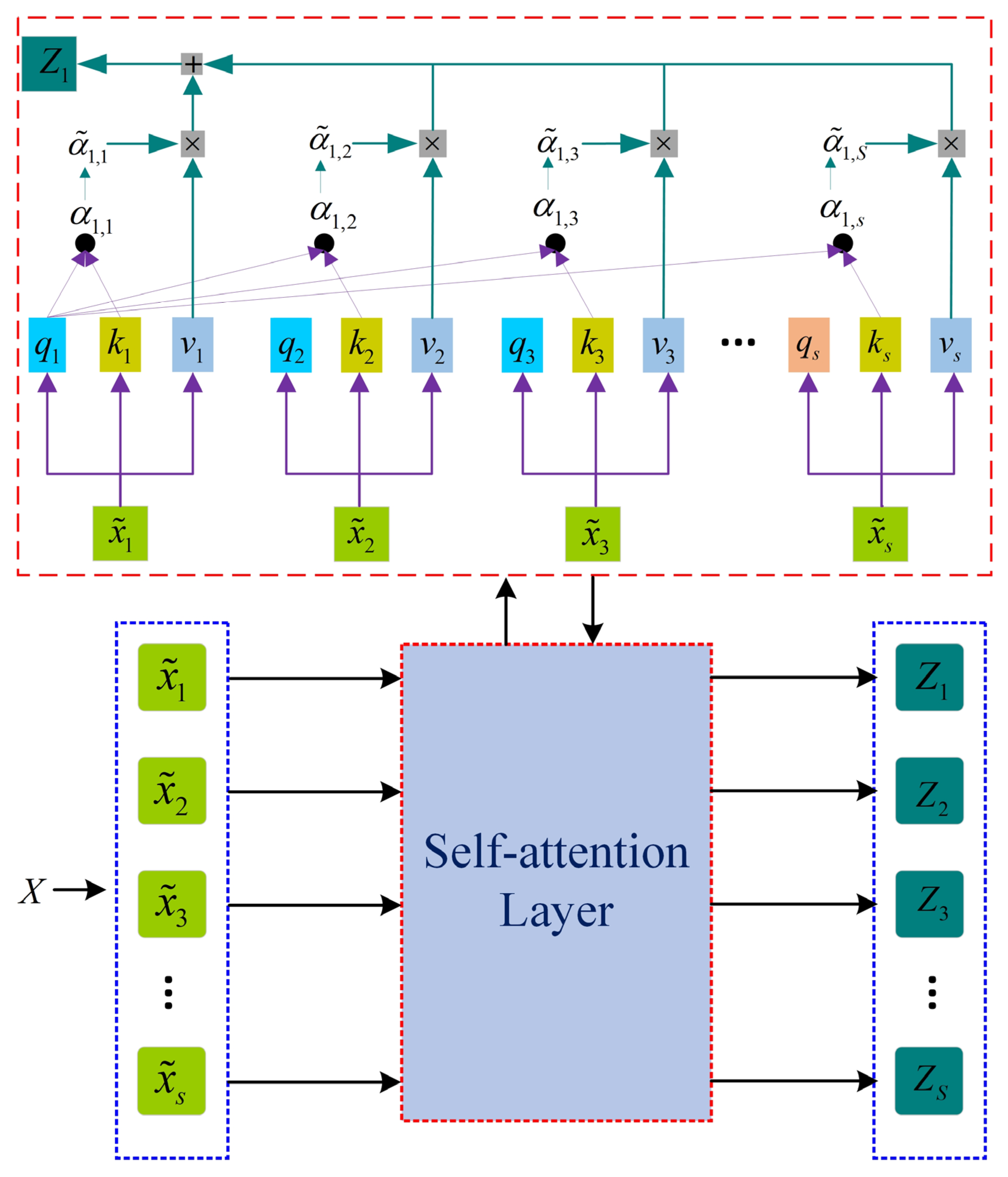
3.2.2. Multi-Headed Self-Attention Mechanism

The working mechanism of Transformer is to selectively focus on the given data for learning. Meanwhile, the function of the self-attention module is to use the observation part of the sample and predict the remaining part. In the encoder structure, the matrices $Q$, $K$, and $V$ are derived from the same input features. The input features are projected to different potential sub-spaces using a learnable feedforward network, which is expressed as Equation (8). A set of queries is packed together into a matrix $Q$, while the keys and values are packed into matrices $K$ and $V$, respectively.

In the self-attention mechanism, $X$ is the input of the input sequence data after embedding. The inputs of an attention module consist of query embedding inputs, key embedding inputs, and value embedding inputs.

According to Equation (8), each vector input to $X$ is multiplied with the three parameter matrices $W^q$, $W^k$, $W^v$, respectively, to calculate their weights. In Figure 8, the red dashed box illustrates the process of calculating the weights of the subsequent input ${\tilde{x}}_1$ and the corresponding output $Z_1$. In order to stabilize the gradient, the weights of the computed serial feature correlations are normalized by dividing them by the square root of dimension $d_k$. After that, the $soft\max$ layer makes the weight matrix into a probability distribution matrix of $\left[0,1\right]$, as in Equations (9)–(11). Then, the weighted $V$ is obtained by multiplying with $v$ at the corresponding position, and the final result is obtained by summing the weighted $V$ values, as in Equation (11). Each of the remaining weight vectors is calculated in a similar manner to $Z_1$. As shown in Figure 8, the advantage of the self-attention mechanism is that it can compute the input sequence in parallel, which greatly improves the speed of extracting the features of the input sequence. Finally, the features $Z_1,Z_2,\cdots Z_s$ of the sequence are extracted quickly and prepared for the subsequent computation.

$$\left\{\begin{array}{l}X{W}^q=Q\\ X{W}^k=K\\ X{W}^v=V\end{array}\right\},$$

(8)

$$\alpha =\left[\begin{array}{ccccc}{\alpha }_{1,1}& {\alpha }_{1,2}& {\alpha }_{1,3}& \cdots & {\alpha }_{1,s}\\ {\alpha }_{2,1}& {\alpha }_{2,2}& {\alpha }_{2,3}& \cdots & {\alpha }_{2,s}\\ {\alpha }_{3,1}& {\alpha }_{3,2}& {\alpha }_{3,3}& \cdots & {\alpha }_{3,s}\\ ⋮& ⋮& ⋮& \cdots & ⋮\\ {\alpha }_{s,1}& {\alpha }_{s,2}& {\alpha }_{s,3}& \cdots & {\alpha }_{s,s}\end{array}\right]=\frac{Q\cdot K^T}{\sqrt{d_k}},$$

(9)

$$\tilde{\alpha }=Soft\max \left(\alpha \right),$$

(10)

$$attention(Q,K,V)=Z={\displaystyle \sum \tilde{\alpha }\cdot V},$$

(11)

where $X$ is the input features, $d_k$ is the dimension of queries and keys, and $W^q$, $W^k$, $W^v$ denote the trainable parameters in different iterative networks. Multi-head attention is also the core component of Transformer.

Multi-head attention uses multiple sets of $W^Q$, $W^K$, $W^V$ to obtain multiple sets of queries, keys, and values, and then each set is computed separately to obtain a $Z$ matrix. Finally, the obtained multiple $Z$ matrices are stitched together.

Benefitting from the multi-head attention operation, the Transformer frame can jointly generate comprehensive latent features of trajectory data from different representation sub-spaces. The multi-head section computes the scaled dot product of each sub-space in parallel and finally concatenates all the attention output according to Equation (12).

$$\{\begin{array}{l}MultiHead(Q,K,V)=concat(hea{d}_1,hea{d}_2,\cdots hea{d}_h){𝒲}^o\\ hea{d}_i=attention(Q{𝒲}_i^Q,K{𝒲}_i^K,V{𝒲}_i^V)\end{array}$$

(12)

where ${𝒲}_i^Q$, ${𝒲}_i^K$, ${𝒲}_i^V$, ${𝒲}_i^O$ are the weight matrices in queries, keys, values, and output.

3.3. Fully Connected Feedforward Layer

A fully connected layer is included in both the encoding and decoding blocks, and the fully connected layer is a two-layer neural network. There is a feedforward network consisting of two linear transformations with a ReLU activation in each sub-layer [20,28], as shown in Equation (13). The fully connected layer is followed by the residual network layer. The residual dropout module is set to reduce overfitting, speed up training, and improve the efficiency of the network.

$$FFN(x)=\mathrm{ReLU}\left(x{W}_1+b_1\right)W_2+b_2,$$

(13)

where $W_1$ and $W_2$ are the weight matrices of fully connected feedforward neural networks.

In the process of data training, the current and previous positions are embedded into the input encoder. The output of the encoder and the output of the LSTM are fused and transmitted together to the decoder section as a memory for attention operation. Thereafter, as the position embedding part of the predicted position vector, the object query information is sent to the decoder part. The decoder recursively and automatically predicts the future position of the trajectory. The decoding process of the decoder is sequential, i.e., when decoding the $i$ vector, it can only be based on the $i-1$ vector and the previous decoding results.

4. Experiments and Results

In this section, experiments are conducted to validate the performance of the proposed model in real ship AIS trajectory prediction. A certain dataset is collected to compare and analyze the prediction performance of different deep learning methods. Several metrics are applied to evaluate the performance of our model and compare it with the current state-of-the-art research methods.

4.1. Dataset Preparation

The data processing procedures and methods are shown in the previous Section 2. The data were collected from the AIS data of vessels in and out of the core port area of Ningbo-Zhoushan, China, between the navigation channel of Luotou and Xiazhimen. Vessels navigating in the waters are mainly merchant vessels for trade transport and there is a high volume of vessel traffic and a variety of vessel types in the waters. The AIS data of ships in the waters are suitable for the validation of the prediction model. The collected data are stored in the form of a database. The AIS data for selected waters are filtered utilizing the defined rectangular boxes with latitude and longitude boundaries. Each row of AIS messages in the database includes the ship’s identifier MMSI, time stamp, latitude and longitude position information, speed, heading, and a static attribute message of the ship. In addition, the AIS transmitting frequency is related to the movement state of the ship. The requirements for the time interval of AIS trajectory points during data processing and the trajectory data with too low speed do not meet the general state of merchant ship navigation in the channel. As a result, we select trajectory data with a speed of more than five knots and a length above ninety meters. Aggregation is also required for the filtered AIS trajectories so that the same identifier (MMSI) AIS data are a collection of independent trajectories in temporal order. Then, the process and method of the time window panning smoothing algorithm for the trajectory data are as in Section 2.1 and will not be repeated here.

4.2. Experimental Design

The main goal of training the model based on the data is to learn the optimal approximation as the prediction result. An effective prediction model can map the spatiotemporal characteristics of trajectories over time based on historical trajectory data. The proposed method is implemented in a Python 3.8-based programming environment. All the algorithms are computed on an NVIDIA RTX 3060 GPU (6GB RAM) platform. The number of encoding and decoding modules in the Transformer framework of the model is set to 6, while the number of multi-heads inside the encoding and decoding modules is set to 8. The number of LSTM layers in the spatiotemporal feature embedding module is set to 3, and the number of nodes in the hidden layer is set to 32. All models are trained by mean square error (MSE) loss function and optimized using the adaptive stochastic gradient descent algorithm Adam. When the learning rate is too large, it will cause the loss function to directly cross the global optimum, and when the learning rate is too small, the loss function will change slowly, which greatly increases the convergence complexity of the model, and it is easy to be trapped in the local optimum, so the learning rate is set to adaptive learning rate = 0.001 in this paper. The variation of the loss in the training and testing sets after 300 epochs of learning the model is shown in Figure 9a. The model gradually converges after 100 epochs of learning, but the loss in the testing set is unstable. When the training exceeds 200 epochs, the loss changes of the training and testing sets tend to be stable. Figure 9b shows the prediction error variation, which quantitatively depicts the prediction effect of the algorithm on longitude and latitude after learning.

4.3. Results

4.3.1. Model Comparison

In order to validate the effectiveness of the proposed algorithm, in this section we compare the prediction results of the proposed algorithm with the LSTM model, Attention-LSTM model, Bi-LSTM mode, and SVR model, respectively. In this section, each model is designed to learn 100 epochs, 200 epochs, and 300 epochs for the data, and then the prediction results are compared, as shown in Figure 10, Figure 11 and Figure 12.

(a) LSTM algorithm trajectory prediction refers to the application of the LSTM method to train the model and predict the longitude and latitude of the trajectory.

(b) Attention-LSTM (abbreviated as LSTM-attn) is the introduction of the attention mechanism in the LSTM method. The essence is to highlight the attention to the features by assigning the difference to the hidden layer units and to predict the features of the trajectory.

(c) The Bi-LSTM model is composed of two LSTM cells with different directions. Information is passed from the positive direction of one cell and the negative direction of the other cell and finally combined into a final output and enables the prediction of trajectory features.

(d) SVR is a support vector regression model, where the core of the model is to find the best linear function and create a spacing band on both sides. The model is optimized by minimizing the total loss and maximizing the support vector.

(e) The comparison shows that the prediction result of the TRFM-LS model is closer to the real value and has a better prediction effect.

4.3.2. Evaluation Metrics

In this study, three indicators, mean absolute error (MAE), mean square error (MSE), and root mean square error (RMSE), are used to evaluate the prediction effectiveness of the model. MAE indicates the mean of the absolute error between the predicted and true values, which can visually reflect the strengths and weaknesses of the model. MSE indicates the expected value of the squared difference between the predicted and true values, and the smaller the value of MSE, the better the prediction model reflects the experimental data with better accuracy. RMSE measures the deviation between predicted and true values, is more intuitive in terms of order of magnitude, and the metric is more sensitive to outliers in the data. The equations are shown in (14)–(16).

$$MAE=\frac{1}{m}{\displaystyle \sum _{i=1}^m\left|y_i-\widehat{y_i}\right|}$$

(14)

$$MSE=\frac{1}{m}{\displaystyle \sum _{i=1}^m{(y_i-\widehat{y_i})}^2}$$

(15)

$$RMSE=\sqrt{\frac{1}{m}{\displaystyle \sum _{i=1}^m{(y_i-\widehat{y_i})}^2}}$$

(16)

where $y_i$ denotes the true value of the trajectory data feature, $\widehat{y_i}$ denotes the corresponding predicted value of the trajectory data feature.

In this section, a statistical method box plot is used to compare the error metrics of the state-of-the-art or typical prediction models. The MAE, MSE, and RMSE are three of the more standardized metrics for evaluating prediction models and are commonly used as metrics in many trajectory prediction studies in the literature. We draw box plots and comparisons of MAE, MSE, and RMSE for each method after trajectory prediction, as shown in Figure 13.

Obviously, the TRFM-LS method has the lowest error metric of MAE of 1.229 for longitude and the lowest error metric of RMSE of 1.584 in terms of prediction performance of ship trajectories. Meanwhile, the error metric of MAE for latitude is as low as 2.131 and that of RMSE is 2.395, both of which are lower than the error metrics of other prediction methods. It demonstrates that the method studied in this paper has better performance in trajectory prediction.

5. Conclusions

The historical AIS trajectory data of ships in busy maritime waters, together with the multi-dimensional features inherent in time series data, provide directions for the scalability of deep learning algorithms used on the data. In this paper, the spatiotemporal correlation of AIS data is fully considered, to mine and exploit their correlation properties. After a multi-dimensional analysis of the data, a time window trajectory filtering method is proposed. The application of this method effectively smooths the jumps and outliers in the trajectory data well, ensures the continuity and integrity of the trajectory, and also prepares the data well for the time series.

This paper integrates a new trajectory time series prediction method based on the deep learning of historical AIS trajectory data of vessels. In the study, the Transformer model is improved based on the characteristics of temporal sequences of trajectory data, and the LSTM module is combined with the Transformer prediction framework. The fused method predicts the position of the ship in the future period. Compared with the state-of-the-art methods, the proposed method in this paper has better prediction accuracy and smaller error, which proves the feasibility and effectiveness of this algorithm. In the gradual development process of intelligent shipping, this research provides a kind of early warning information reference for the ship’s autonomous navigation and collision avoidance.

6. Discussion

6.1. Limitations

This paper explores a new trajectory prediction method by combining the LSTM module and Transformer model based on deep learning theory, but there are some limitations in this research. The predicted trajectory is the vessel’s track data under normal navigation conditions and does not take into account the effects of external factors such as special weather conditions and encounters with other vessels. In addition, the preprocessing of the data is based on spatiotemporal characteristics to establish the time series data.

6.2. Future Research

Future research could be conducted to address the above limitations. For example, the prediction of multi-dimensional features of trajectories based on deep learning methods when considering ship encounter scenarios. Alternatively, deep learning models could be used as a basis for studying the prediction of trajectory data and ship dynamics characteristics after being influenced by geographical and meteorological conditions.

References

1. Rødseth, Ø.J.; Perera, L.P.; Mo, B. Big Data in Shipping—Challenges and Opportunities. In Proceedings of the 15th International Conference on Computer Applications and Information Technology in the Maritime Industries (COMPIT 2016), Lecce, Italy, 9–11 May 2016. [Google Scholar]
2. Liu, H.; Jurdana, I.; Lopac, N.; Wakabayashi, N. BlueNavi: A Microservices Architecture-Styled Platform Providing Maritime Information. Sustainability 2022, 14, 2173. [Google Scholar] [CrossRef]
3. Jurdana, I.; Lopac, N.; Wakabayashi, N.; Liu, H. Shipboard Data Compression Method for Sustainable Real-Time Maritime Communication in Remote Voyage Monitoring of Autonomous Ships. Sustainability 2021, 13, 8264. [Google Scholar] [CrossRef]
4. Chen, P.; Li, M.; Mou, J. A Velocity Obstacle-Based Real-Time Regional Ship Collision Risk Analysis Method. J. Mar. Sci. Eng. 2021, 9, 428. [Google Scholar] [CrossRef]
5. Schmidhuber, J. Deep learning in neural networks: An overview. Neural Netw. 2015, 61, 85–117. [Google Scholar] [CrossRef] [PubMed]
6. Zaman, B.; Marijan, D.; Kholodna, T. Interpolation-Based Inference of Vessel Trajectory Waypoints from Sparse AIS Data in Maritime. J. Mar. Sci. Eng. 2023, 11, 615. [Google Scholar] [CrossRef]
7. Zhao, S.; Tang, C.; Liang, S.; Wang, D. Track prediction of vessel in controlled waterway based on improved Kalman filter. J. Comput. Appl. 2012, 32, 3247–3250. [Google Scholar] [CrossRef]
8. Zhang, Z.; Ni, G.; Xu, Y. Trajectory prediction based on AIS and BP neural network. In Proceedings of the 2020 IEEE 9th Joint International Information Technology and Artificial Intelligence Conference (ITAIC), Chongqing, China, 11–13 December 2020; pp. 601–605. [Google Scholar]
9. Sørensen, K.A.; Heiselberg, P.; Heiselberg, H. Probabilistic Maritime Trajectory Prediction in Complex Scenarios Using Deep Learning. Sensors 2022, 22, 2058. [Google Scholar] [CrossRef] [PubMed]
10. Murray, B.; Perera, L.P. A dual linear autoencoder approach for vessel trajectory prediction using historical AIS data. Ocean Eng. 2020, 209, 107478. [Google Scholar] [CrossRef]
11. Gupta, A.; Johnson, J.; Li, F.F.; Savarese, S.; Alahi, A. Social GAN: Socially Acceptable Trajectories with Generative Adversarial Networks. In Proceedings of the 2018 IEEE/CVF Conference on Computer Vision and Pattern Recognition (CVPR), Salt Lake City, UT, USA, 18–23 June 2018. [Google Scholar]
12. Zhang, Z.; Ni, G.; Xu, Y. Ship Trajectory Prediction based on LSTM Neural Network. In Proceedings of the 2020 IEEE 5th Information Technology and Mechatronics Engineering Conference (ITOEC), Chongqing, China, 12–14 June 2020; pp. 1356–1364. [Google Scholar]
13. Ding, M.; Su, W.; Liu, Y.; Zhang, J.; Li, J.; Wu, J. A Novel Approach on Vessel Trajectory Prediction Based on Variational LSTM. In Proceedings of the 2020 IEEE International Conference on Artificial Intelligence and Computer Applications (ICAICA), Dalian, China, 27–29 June 2020; pp. 206–211. [Google Scholar]
14. Bao, K.; Bi, J.; Gao, M.; Sun, Y.; Zhang, X.; Zhang, W. An Improved Ship Trajectory Prediction Based on AIS Data Using MHA-BiGRU. J. Mar. Sci. Eng. 2022, 10, 804. [Google Scholar] [CrossRef]
15. Wang, R.; Peng, C.; Gao, J.; Gao, Z.; Jiang, H. A dilated convolution network-based LSTM model for multi-step prediction of chaotic time series. Comput. Appl. Math. 2020, 39, 30. [Google Scholar] [CrossRef]
16. Gao, D.; Zhu, Y.; Zhang, J.; He, Y.; Yan, K.; Yan, B. A novel MP-LSTM method for ship trajectory prediction based on AIS data. Ocean Eng. 2021, 228, 108956. [Google Scholar] [CrossRef]
17. Capobianco, S.; Millefiori, L.M.; Forti, N.; Braca, P.; Willett, P. Deep Learning Methods for Vessel Trajectory Prediction Based on Recurrent Neural Networks. IEEE Trans. Aerosp. Electron. Syst. 2021, 57, 4329–4346. [Google Scholar] [CrossRef]
18. Bai, S.; Kolter, J.Z.; Koltun, V. An Empirical Evaluation of Generic Convolutional and Recurrent Networks for Sequence Modeling. arXiv 2018, arXiv:1803.01271. [Google Scholar]
19. Giuliari, F.; Hasan, I.; Cristani, M.; Galasso, F. Transformer Networks for Trajectory Forecasting. In Proceedings of the 2020 25th International Conference on Pattern Recognition (ICPR), Milan, Italy, 10–15 January 2021; pp. 10335–10342. [Google Scholar] [CrossRef]
20. Vaswani, A.; Shazeer, N.; Parmar, N.; Uszkoreit, J.; Jones, L.; Gomez, A.N.; Kaiser, L.; Polosukhin, I. Attention Is All You Need. In Advances in Neural Information Processing Systems 30 (NIPS 2017), Proceedings of the 31st Annual Conference on Neural Information Processing Systems (NIPS), Long Beach, CA, USA, 4–9 December 2017; Guyon, I., Luxburg, U.V., Bengio, S., Wallach, H., Fergus, R., Vishwanathan, S., Garnett, R., Eds.; Neural Information Processing Systems Foundation: La Jolla, CA, USA, 2017; Volume 30. [Google Scholar]
21. Brown, T.B.; Mann, B.; Ryder, N.; Subbiah, M.; Kaplan, J.; Dhariwal, P.; Neelakantan, A.; Shyam, P.; Sastry, G.; Askell, A.; et al. Language models are few-shot learners. In Proceedings of the Neural Information Processing Systems Foundation, Vancouver, BC, Canada, 6–12 December 2020; Available online: https://dl.acm.org/doi/abs/10.5555/3495724.3495883 (accessed on 16 March 2023).
22. Sun, G.; Zhang, C.; Woodland, P.C. Transformer Language Models with LSTM-Based Cross-Utterance Information Representation. In Proceedings of the ICASSP 2021–2021 IEEE International Conference on Acoustics, Speech and Signal Processing (ICASSP), Toronto, ON, Canada, 6–11 June 2021; pp. 7363–7367. [Google Scholar]
23. Dai, Z.; Yang, Z.; Yang, Y.; Carbonell, J.; Le, Q.; Salakhutdinov, R. Transformer-{XL}: Attentive Language Models beyond a Fixed-Length Context; Association for Computational Linguistics-ACL: Florence, Italy, 2019; pp. 2978–2988. [Google Scholar]
24. Beltagy, I.; Peters, M.E.; Cohan, A. Longformer: The Long-Document Transformer. arXiv 2020, arXiv:2004.05150. [Google Scholar]
25. Cai, L.; Janowicz, K.; Mai, G.; Yan, B.; Zhu, R. Traffic transformer: Capturing the continuity and periodicity of time series for traffic forecasting. Trans. GIS 2020, 24, 736–755. [Google Scholar] [CrossRef]
26. Fan, C.; Zhang, Y.; Pan, Y.; Li, X.; Zhang, C.; Yuan, R.; Wu, D.; Wang, W.; Pei, J.; Huang, H.; et al. Multi-Horizon Time Series Forecasting with Temporal Attention Learning. In Proceedings of the KDD’19: 25th Acm Sigkdd International Conferencce on Knowledge Discovery and Data Mining (KDD), Anchorage, AK, USA, 4–8 August 2019; pp. 2527–2535. [Google Scholar]
27. Cinar, Y.G.; Mirisaee, H.; Goswami, P.; Gaussier, E.; Ait-Bachir, A.; Strijov, V. Position-Based Content Attention for Time Series Forecasting with Sequence-to-Sequence RNNs. In Neural Information Processing, Proceedings of the ICONIP 2017 24th International Conference on Neural Information Processing (ICONIP), Guangzhou, China, 14–18 November 2017; Liu, D., Xie, S., Li, Y., Zhao, D., ElAlfy, E., Eds.; Springer: Cham, Switzerland, 2017; Volume 10638, pp. 533–544. [Google Scholar] [CrossRef]
28. Fan, Z.; Gong, Y.; Liu, D.; Wei, Z.; Wang, S.; Jiao, J.; Duan, N.; Zhang, R.; Huang, X. Mask Attention Networks: Rethinking and Strengthen Transformer. arXiv 2021, arXiv:2103.13597. [Google Scholar]
Figure 1. Vessel traffic patterns in Ningbo-Zhoushan waters. (a) AIS density map of vessel data within the geographic box (b) AIS traffic flow pattern distribution of vessels in predefined areas.
Jmse 11 00880 g001
Figure 2. Trajectory before time window panning and smoothing filtering: (a) Vessel trajectory in the geographical area before filtering, the arrows point out the jagged or rippled localization in the anomalous trajectory (b) Mapping of parts of anomalous trajectories in a geographical area.
Jmse 11 00880 g002
Figure 3. Time window panning and smoothing filtering schematic: (a) Schematic diagram of the trajectory filtering process (b) Diagram of trajectory filtering before and after.
Jmse 11 00880 g003
Figure 4. Trajectory after time window panning and smoothing filtering: (a) Vessel trajectory in the geographical area after filtering (b) The mapping of part of the anomalous trajectory after smoothing.
Jmse 11 00880 g004
Figure 5. Data Processing Flow Chart.
Jmse 11 00880 g005
Figure 6. The Transformer Structure.
Jmse 11 00880 g006
Figure 7. LSTM Cell Diagram.
Jmse 11 00880 g007
Figure 8. Frame Diagram of the Attention Mechanism.
Jmse 11 00880 g008
Figure 9. Loss curve and prediction error: (a) Loss variation of the model (b) The prediction error variation.
Jmse 11 00880 g009
Figure 10. The comparison of the performance after learning 100 epochs of different methods: (a) LSTM (b) LSTM-attn (c) Bi-LSTM (d) SVR (e) TRFM-LS.
Jmse 11 00880 g010
Figure 11. The comparison of the performance after learning 200 epochs of different methods: (a) LSTM (b) LSTM-attn (c) Bi-LSTM (d) SVR (e) TRFM-LS.
Jmse 11 00880 g011
Figure 12. The comparison of the performance after learning 300 epochs of different methods: (a) LSTM (b) LSTM-attn (c) Bi-LSTM (d) SVR (e) TRFM-LS.
Jmse 11 00880 g012
Figure 13. Metrics comparison of different methods: (a) Comparison of MAE predicted by different methods (b) Comparison of MSE predicted by different methods (c) Comparison of RMSE predicted by different methods.
Jmse 11 00880 g013
Disclaimer/Publisher’s Note: The statements, opinions and data contained in all publications are solely those of the individual author(s) and contributor(s) and not of MDPI and/or the editor(s). MDPI and/or the editor(s) disclaim responsibility for any injury to people or property resulting from any ideas, methods, instructions or products referred to in the content.