Article

Predictive Control of a Heaving Compensation System Based on Machine Learning Prediction Algorithm

1
Ulsan Ship and Ocean College, Ludong University, Yantai 264025, China
2
Department of Naval Architecture, Ocean and Marine Engineering, University of Strathclyde, Glasgow G4 0TD, UK
3
College of Transporation, Ludong University, Yantai 264025, China
4
Yantai Research Institute, Harbin Engineering University, Yantai 264006, China
*
Author to whom correspondence should be addressed.
J. Mar. Sci. Eng. 2023, 11(4), 821; https://doi.org/10.3390/jmse11040821
Submission received: 21 March 2023 / Revised: 9 April 2023 / Accepted: 11 April 2023 / Published: 12 April 2023
(This article belongs to the Topic Control and Optimisation for Offshore Renewable Energy)

Abstract

:
Floating structures have become a major part of offshore structure communities as offshore engineering moves from shallow waters to deeper ones. Floating installation ships or platforms are widely used in these engineering operations. Unexpected wave-induced motions affect floating structures, especially in harsh sea conditions. Horizontal motions on the sea surface can be offset by a dynamic positioning system, and heave motions can be controlled by a heave compensation system. Active heave compensation (AHC) systems are applied to control vertical heave motions and improve safety and efficiency. Predictive control based on machine learning prediction algorithms further improves the performance of active heave compensation control systems. This study proposes a predictive control strategy for an active heave compensation system with a machine learning prediction algorithm to minimise the heave motion of crane payload. A predictive active compensation model is presented to verify the proposed predictive control strategy, and proportion–integration–differentiation control with predictive control is adopted. The reliability of back propagation neural network (BPNN) and long short-term memory recurrent neural network (LSTM RNN) prediction algorithms is proven. The influence of the predictive error on compensation performance is analysed by comparing predictive feedforward cases with actual-data feedforward cases. Predictive feedforward control with regular and irregular wave conditions is discussed, and the possible strategies are examined. After implementing the proposed predictive control strategy based on a machine learning algorithm in an active heave compensation system, the heave motion of the payload is reduced considerably. This investigation is expected to contribute to the motion control strategy of floating structures.

1. Introduction

Offshore engineering has moved from shallow waters to deeper ones, and floating structures have become a major part of offshore engineering communities. Ship and ocean engineering platforms are affected by wave load, so undesirable motions affect many engineering operations [1], including the equipment handling of oil and gas systems [2], floating wind turbine installations [3], and equipment recovery [4]. Hence, high-quality operability is required in harsh sea conditions. Horizontal motions on the sea surface can be offset by a dynamic positioning (DP) system, which is actuated by a propeller in two directions. Relative heave motion is controlled by a compensation system. A compensation system has been developed from passive compensation to active compensation [5]. One of the most important applications of the heave compensation system is the crane systems of loading ships. In terms of the safety and efficiency of production loading in harsh sea conditions, the crane system controls the velocity, load and displacement of payload to minimise the operational download time or vibration [6].
Controlling the vertical motion of the payload is important in keeping the loading operation safe and efficient. The wave-induced motion of a ship leads to critical tension of the rope [7], which should not be less than zero to avoid slack rope situations, and the rope should not exceed the safety limit to avoid unrecoverable damage. Large undesirable motions between the payload and ship pose a potential danger, and unexpected motions are important causes of loading inefficiency. One of the objectives of heave compensation is to decouple wave/wind-induced motion from payload motion for the payload to move smoothly in an expected manner. Compensation systems are divided into two categories: passive heave compensation (PHC) and active heave compensation (AHC). PHC works as a vibration isolator placed between the payload and ship. It is regarded as a spring–damper system that restores and releases energy to offset the wave-induced heave motion. Hatleskog and Dunnigan (2006) simulated a PHC and showed that a passive compensator can reduce the effects of heave in deep water but only to a limited extent [8]. It is inefficient for many complex applications that require accurate compensation or involve the relative motions of two bodies. Hence, AHC is proposed to obtain enhanced performance by detecting the heave motion of the ship and transmitting the detected information to the controller; the controller then makes corresponding actions to achieve compensation. Küchler et al. (2010) used a feedforward controller with predicted motion to compensate for heave motion. The proposed controller and the prediction algorithm decouple the motion of the rope-suspended payload from the vessel’s motion. The active compensation system can achieve enhanced compensation effects by collecting ship motion information [9]: the heave motion of the ship is measured and fed back to a compensation controller [10]. Woodacre et al. (2015) conducted a comprehensive review of heave compensation, especially in underwater conditions, and established a future development direction of AHC systems.
The control accuracy of floating structures can be improved by eliminating the time delay of the control system. Many researchers have studied the prediction of heave motion. Shi et al. (2014) presented a crane active heave prediction modelling method based on a support vector machine (SVR) for regression, and the parameters of the SVR were optimised by the particle swarm algorithm to improve heave motion prediction accuracy [11]. Ngo et al. (2017) proposed a fuzzy sliding mode control strategy combined with a prediction algorithm based on Kalman filtering to suppress the sway motion of the payload [12]. Least squares SVM has also been improved by an artificial immune algorithm to predict the motion trend of offshore platforms [13]. Through the prediction of heave motion, the short-term motion state can be effectively obtained and used as the input of the control system. To acquire the best control scheme, proportion–integration–differentiation (PID) control [14] and fuzzy PID control [15] have been widely used in engineering. Moreover, the back propagation (BP) neural network PID control method [16] has been adopted to perform simulation analyses because the neural network has self-learning capabilities. An increasing number of machine learning algorithms have been introduced to control strategies for prediction and control parameter optimisation in recent years [17,18].
In summary, heave motion prediction plays an important role in the AHC system. Many control strategies have been used in heave compensation systems regardless of whether feedback or feedforward control is involved. PID control is a control loop mechanism that employs feedback, and it is widely used in offshore compensation control systems [19]. A PID controller continuously calculates the error value as the difference between a desired set point and a measured process variable. Then, it applies correction based on three terms: proportional, integral and differential terms. Thus, PID control has the advantages of simple principle, convenience of utility, good stability and robustness [20]. As one of the most frequently used and efficient methods, it is implemented to minimise the load motion. The predictive control strategy is a tool for optimising the performance of offshore heave compensation systems, especially when it is coupled with advanced machine learning techniques. With the predicted information of wave-induced motion, the phase lag is expected to be eliminated. The BP neutral network can approximate any nonlinear function, so its structure and learning algorithm are simple and clear [21]. Long short-term memory recurrent neural network (LSTM RNN) algorithms are the most popular type of RNN, and they can help overcome diminishing or exploding gradients during the training process [22]. They can be used to adjust and optimise PID controller parameters in accordance with the system state. Therefore, this study proposes an active heave compensation system with PID based on machine learning prediction algorithms (BPNN and LSTM RNN) which use predicted motions to minimise the deviation of the heave compensation system. The accuracies of different machine learning prediction algorithms with regular and irregular wave conditions are compared, and the influence of the predictive motion data and actual-data feedforward cases on compensation performance is analysed. The rest of the paper is organised as follows. Section 2 briefly addresses the AHC system and the modelling process. A simplified heave compensation model is presented to focus on the design predictive controller. Machine learning prediction algorithms, namely, BPNN and LSTM RNN, are introduced, and a predictive PID control strategy is developed. In Section 3, predictive feedforward control under regular structure motion is analysed. In Section 4, predictive feedforward control under irregular structure motion is investigated and compared with regular structure motion. The conclusions are presented in Section 5.

2. Control Strategy of the Heave Compensation System

2.1. Heave Compensation Model

For a crane on a ship or floating platform, the heave compensation system contains a series of complex components, such as the controller, ropes, actuator and motor. The present study focuses on the design of AHC predictive control and makes some assumptions to simplify the mechanism. The compensation mechanism is regarded as an integrated unit, and the control command is the variable force of the rope. Hence, the heave motion compensation system is not influenced by the DP system that is used to modify the horizontal loading motions of the ship. The motion reference unit (MRU) collects motion information. It is assumed to directly collect heave motions between two bodies that have been decoupled from the multi-degree-of-freedom motions.
The active heave compensation system described in this paper is shown in Figure 1. In this paper, the motion of the floating structure is called the reference motion. The motion of the payload is the compensated motion because the motion of the payload is controlled by AHC. The displacement of the rope is the response motion of the controller. From the view of the control system, the relative heave motion in each time step is the input of the compensation system, namely, the set point. Given that the deformation of the rope is disregarded here, the displacement of the rope is set as the process variable, which is compensated to the payload. The actual heave motion of the payload is the error in the control loop. The dynamic model of the crane is expressed as
d v d t = F m d z d t = v ,
where F is the force of the payload in the heave direction and m is the mass of the payload. In the form of state space representation, Equation (1) can be rewritten as
x 1 = z x 2 = v u = F m x ˙ 1 x ˙ 2 = 0 1 0 0 x 1 x 2 + 0 1 u y = 1 0 x 1 x 2 + 0 u ,
where z is the vertical displacement of the payload, v is the vertical velocity of the payload, u is the input variable of the compensation system, y is the output variable and x is the state vector with a dimension of 2 × 1 .
The whole control process is illustrated in Figure 2, which combines PID control and motion prediction into an integrated system. The block that represents the predicted heave motion is different from the feedback PID control. This block contains the predictive machine learning algorithm to optimise the performance of the compensation system.

2.2. Prediction Methodology

Feedback control is inevitably influenced by phase lagging in the control process. Actuation implementation needs time to react even though the measured variable is perfect, so feedback control cannot perform optimally in real-time applications. If the motion is known or can be predicted in advance, the effect caused by actuation time can be eliminated. Predictive control helps offset the lag with an accurate prediction algorithm. With the simplicity of the compensation system, the next step of the predictive control study is to address the prediction method of the future motion of the floating structure. In practical applications, the floating structure is a complex system that may be combined with other dynamic systems, such as mooring or DP systems. Moreover, the system changes because of ageing, malfunction, uploading and downloading. Analysing the system under every condition is difficult. By learning from the historical behaviour of the floating structure on waves, the relationship between the wave motion and floating structure can be expressed in an approximate form in the neural network. Two types of supervised machine learning algorithms, namely, BPNN and LSTM RNN, are introduced to predict the future heave motion of the loading ship.

2.2.1. BPNN

The BPNN shown in Figure 3 is a basic class of the artificial neural network (ANN) community. Three types of layers describe the state of data, and the nonlinear transformation between layers is processed with the activation function. The left and right layers store the input and output data. The hidden layer in the middle expresses the process of nonlinear transformation with the neural network activation function. The perception units of BPNN simulate the information transformation through brain neurons as follows:
z k l = σ ( ξ k l ) ξ k l = k = 1 n ( w k ( l 1 ) · z k ( l 1 ) + b ( l 1 ) ) l = 2 , 3 , , N ,
where z k l is the output (heave motion of BPNN); ξ k l is the input (wave elevation); the subscripts k and l represent the layer and neuron numbers in the complex deep learning neural network, respectively; and σ is the activation function. For the hidden layers, σ is the sigmoid function, and for the output layer, σ is a linear function. w is the weight, and b is the bias. The error propagation is a convex optimisation problem that is solved by back propagation and gradient descent [23].

2.2.2. LSTM RNN

BPNN is the most basic architecture of the ANN community and has an advanced class for specific fields. With multi-layer BPNN, the majority of general requirements can be met, and advanced techniques have been developed to push the limitations of BPNN to high-nonlinearity or high-dimensional cases. In this section, a novel LSTM RNN is introduced to predict time-series motions. The memory block in Figure 4 is the basic unit of LSTM RNN, and it includes the input gate, output gate, forget gate and state cell. These gates and cells exchange information through the constant error carousel to ‘keep memory’ of the characteristics in the time series. The gates control the information flow and transmit information between short-term memory and long-term memory. The state cell stores the long-term memory of the time series process. The new input enters the memory block and becomes the long-term memory after a series of nonlinear transformations. LSTM RNN is regarded as a deep learning architecture because of the existence of the memory block. Therefore, LSTM RNN is the professional solution for time-series processes.
f t = σ ( z f ) = σ ( ω f · ξ + b f ) i t = σ ( z i ) = σ ( ω i · ξ + b i ) o t = σ ( z o ) = σ ( ω o · ξ + b o ) c ˜ t = tanh ( z c ˜ ) = tanh ( ω c · ξ + b c ) c t = f t × c t 1 + i t × c ˜ t h t = o t × tanh ( c t ) ,
where the subscripts, f , i , o represent the forget gate, input gate and output gate, respectively; σ is the sigmoid function and the activation function in different types of neural networks; and tanh is the hyperbolic tangent function. The operator × is defined as the multiple operations of matrices and vectors [24]. The information transforms not only through the layers but also through time. In BPNN, the error propagation through layers is the only factor considered. Meanwhile, in LSTM RNN, the error propagations through layers and time steps are considered simultaneously. The error propagation algorithm is called back propagation through time.

2.3. Predictive PID Control

The future motion is predicted based on a machine learning algorithm, and the predicted motion is treated as the set point of the current time step in the PID control loop. The feedback PID control law is expressed as
u ( t ) = k p e ( t ) + k i 0 t e ( τ ) d τ + k d d e ( t ) d t ,
where u is the control command output of the controller and the input vector of the heave compensation system shown in Equation (2); k p , k i and k d are the proportional gain, integral gain and differential gain, respectively; e is the deviation signal; and t is the time duration of the whole control process. The discrete form of the numerical simulation process is expressed as
u ( k ) = k p e ( k ) + k i j = 0 k e ( k ) Δ t + k d e ( k ) e ( k 1 ) Δ t ,
e ( k ) = z m ( k ) z u ( k ) ,
where Δ t is the sampling, k is the sampling number, z m is the heave motion measured by MRU and z u is the controller response of the heave compensation system. Equations (6) and (7) are only for cases where all motion is the actual value in each sampling step. When the predicted motion of the machine learning algorithm is used in the control strategy, the equation is updated to replace the measured motion with the predicted motion in the PID control system.
u ( k ) = k p e p ( k ) + k i j = 0 k e ( k ) Δ t + k d e p ( k ) e ( k 1 ) Δ t ,
e p ( k ) = z p ( k ) z u ( k )
where e p is the calculated error between the predicted motion and controller response motion of AHC and z p is the predicted motion ahead of the current motion. Only proportional and differential terms need to be updated due to the existence of the predicted motion, and the integral term is not influenced by the predictive information because the integral term only reflects the history accumulation effect of the control process.

2.4. Data Processing

Given that the performance of machine learning prediction is influenced by the quality of statistics, pre-processing is necessary to improve the accuracy and efficiency of the prediction algorithm. Dataset normalization is shown below, and it covers the range of [−1, 1].
z = 2 ( Z Z min Z max Z min ) 1 ,
where Z is the deformalized input and z is the normalized input. The subscripts max and min are the maximum and minimum values of the input data, respectively. Normalization of input and output data is not only beneficial to network training, as it eliminates the errors caused by different magnitudes of inputs, but also allows for the comparison of the prediction and control performance from different methods or sea conditions. At the same time, the values of the control command can be inverse-normalized mathematically in practical applications.
In this study, the results of the control strategy with actual information are called actual-data feedforward motion, and the results of the control strategy with prediction information are called prediction motion. For example, one-step actual-data feedforward means that the control process involves one step of the actual future heave motion, and two-step BPNN/LSTM prediction means that the control result considers the influence of two-steps-ahead heave information. If no future information is involved in the PID control process, that is, common feedback control, then the performance without feedforward is compared with the performance with feedforward and prediction. To verify the predictive control strategy, the performance is evaluated with the deviation form of mathematical statistics analysis. Mean absolute error (MAE) and root mean square error (RMSE) are used to describe the accuracy of the response results in this study.
M A E = 1 N 1 N z z ^ ,
RMSE = 1 N z z ^ 2 N ,
where z is the predicted value of heave motion, z ^ is the actual data value of heave motion and N is the quantity of the prediction data. The performance of cases is compared based on these statistical errors. The smaller these errors are, the better the performance is.

3. Predictive Feedforward Control under Regular Structure Motion

The study starts from regular motion cases, then extends to irregular motion cases. The reference heave motion of a sinusoidal signal that has been normalized is depicted in Figure 5. The normalized amplitude is 1, and the frequency of the structure motion is 0.25 Hz. The sampling frequency of the reference heave motion is 10 Hz, which means that the feedforward frequency is 10 Hz as well. The heave motions of the compensation unit based on feedback and feedforward control are compared in the same figure. The reference motion is the compared target to evaluate the performance of different strategies qualitatively. In the case without feedforward control, although the response motion behaves in the same period and at the same amplitude as the reference motion, a response lag still exists between the reference motion and the controller response motion. The reason is that feedback control regards only the current reference motion as the control input. The response does not consider the compensation component in the next step in advance. Therefore, an inherent delay exists because of the nature of the feedback control strategy. To reduce the influence of response time lag as much as possible, the influence of future information in the control system is considered by the feedforward control strategy, thus reducing the time lag and amplitude of load motion compared with feedback control.

3.1. Actual-Data Feedforward Control

First, the compensation effect of actual-data feedforward control is analysed before the predicted data are involved. The reference structure motion and the response motion are compared, and the phase shift is illustrated clearly in Figure 5. When the forward step rises from 0 (which is equivalent to feedback control) to 1, the time lag decreases considerably. The closer the response motion is to the reference motion, the more accurate the performance is. A similar phenomenon is also observed in the two-step feedforward case, where the heave motion response is only slightly ahead of the reference heave motion. However, when the number of steps ahead increases to 3, the performance of AHC is worse than that of the two-step feedforward case because the phase shift of feedforward control is larger in this case. In general, the response motions of the control system appear to translate from right to left (from lagging to ahead). When the two-step feedforward control is implemented, the effect of heave compensation control is the best of all listed cases.
The heave motions of the payload that can be compensated by feedforward control are shown in Figure 6. When the reference motion is normalized to [−1, 1], even in the worst cases (cases without feedforward and three-step feedforward control), the amplitudes decreases to about 30%. Comparison of the phase shift shows no significant difference between the one-step and two-step feedforward control. However, the amplitude of load heave motion in the two-step feedforward case is almost half of that in the one-step feedforward case. When the phase shift changes from lagging to ahead, the peak appears in a certain moment, such as 2.0 s, and is then converted to a valley. Overall, in consideration of both phase shift and amplitude reduction, two-step feedforward control with actual-data future information is the best choice for the proposed heave compensation system.

3.2. BPNN Feedforward Control

The actual-data feedforward control analysis shows that two-step feedforward control is the best option. The next step is to determine how proximate predictive machine learning algorithms influence the performance of the control system. Although the two-step feedforward case is the optimal choice when the future information is actual, whether that conclusion is affected when the future information is predicted remains unknown. The actual-data and prediction cases with the same feedforward steps are called corresponding cases. In this study, the future motion is predicted based on two machine learning algorithms: BPNN and LSTM RNN. As shown in Figure 7, BPNN prediction has the same accuracy as LSTM prediction. No significant difference is observed between BPNN and LSTM RNN prediction motions for a single harmonic motion. However, the trade-off between time consumption and accuracy is considered here because BPNN is less time-consuming than LSTM RNN. Thus, in the regular structure motion section, only the BPNN prediction results are discussed, but the discussion is suitable for LSTM prediction.
On the basis of prediction feedforward control, Figure 8 shows the controller response motions to a sinusoidal signal. Figure 9 shows the heave motion of the payload. As shown in Figure 8 and Figure 9, the tendencies of phase deviation and compensated payload motion are similar to those in the actual-data feedforward cases. The different deviation types of amplitudes, phases and errors are listed in Table 1, which includes actual-data and prediction feedforward cases. The difference in amplitude between the actual-data and prediction feedforward cases is only 0.01. Given that the reference amplitude is 1, the 1% difference can be ignored. Therefore, the predicted information based on the machine learning algorithm is reliable. The control strategy of using predicted data performs almost the same as that of using actual data. To compare the phase deviation quantitatively in a discrete form, the lagging step number is defined as follows:
n = t l a g T s ,
where t l a g is the length of lagging time, that is, the time gap between the peaks of reference motion and controller response motion; T s is the sampling period or the inverse number of sampling frequency; and n is the lagging step number, which is an integer. When n is positive, the response lags behind the reference motion; when n is negative, the response is ahead of the reference motion.
Except for the case where the phase lag of one-step prediction is smaller than that of the one-step actual-data feedforward case, the other corresponding cases have the same lagging step number. MAE and RMSE initially decrease and then increase, and they present the same tendency as the maximum amplitude. A comparison of these deviations is shown in Figure 10. The analysis of the deviations shows that replacing the actual motion with the well-predicted motion is feasible when the future information is unknown.

3.3. Analysis of Optimal Forward Steps

Predicted motion based on BPNN has been proven to be an alternative variable when the future motion is unknown in a certain case. If the number of prediction steps is insufficient (0 or 1) or excessive (3 steps), it decreases the accuracy, as shown in Figure 11. To determine the optimal steps for different regular sea conditions and compare the influence of sampling frequency and structure motion frequency, two kinds of sampling frequency ω s (10 and 100 Hz), five kinds of motion frequency ω m (1, 2, 4, 8 and 16 Hz) and six kinds of step number k (0, 1, 2, 3, 4 and 5) are selected to accomplish a series of payload motion calculations. The most common frequency of structure motion is about 0.1–1 Hz. A sampling frequency that is more than 10 times the structure motion has been proven to be reasonable via experimental tests or operational devices because the characteristics are collected precisely. If the sampling frequency is fixed at 10 Hz and the motion frequency increases from 1 Hz to 16 Hz, the measured data will become less precise. Thus, inaccuracy sampling measurement is also considered in this study. Given that MAE and RMSE reflect the same trend as amplitude does, only amplitude and phase deviation are analysed; discussions of MAE and RMSE are not repeated in this section. Table 2, Table 3, Table 4 and Table 5 show the calculated results of different simulated cases.
As shown in Figure 11, when forward step number k rises from 0 to 1, the maximum amplitudes of payload motion decrease to 40% for all frequencies of structure motion. The reduction in the maximum amplitude is only 20% from 1 step to 2 steps in the case of the 0.0625 Hz structure motion, and this ratio increases to 36% if the frequency of structure motion ω m is 1 Hz. When the frequency of structure motion ω m increases, the motion varies more quickly than it does under a low frequency. Therefore, the control feedback does not compensate for as much motion as the low-frequency cases do. From the two-step to five-step cases, the payload motions increase in a linear manner. For the four-step and five-step cases, the amplitudes of load motion exceed that of feedback control. In the case of ω s = 100 Hz and ω m = 1 Hz, the amplitudes of the one-step and two-step cases are almost equal.
The adopted control approach is a PID controller which is sensitive to errors from the set point. The two-forward steps leave a distance deviation to generate a suitable control force to minimize the distance gaps. When k is less than 2, the control response is insufficiently large to compensate for the heave motion. When k is larger than 2, the future motion is overestimated, which causes overshoot of the compensation. The higher the frequency of the structure motion, the larger the overshoot of the control result. Therefore, two-step-forward prediction is beneficial for low-frequency structure motion. However, for high-frequency structure motion, two-step-forward prediction is unnecessary because no significant improvement can be achieved.
As shown in Figure 12, the variable of the vertical axis is A m p max · ω s / ω m , and it is treated as the amplitude growth speed of motion frequency. When the sampling frequency is 100 Hz (warm-colour cases), the curves are constant values. This situation means that the relationships between the payload amplitudes and motion frequencies are linearly proportional. When the sampling frequency is 10 Hz (cold-colour cases), the amplitude growth speed drops with the increase in motion frequency in the 0-, 1-, 4- and 5-step cases. If the number of prediction steps is 2 or 3, the amplitude growth speed will increase with the increase in motion frequency. In other words, the performance of good models worsens, whereas the performance of poor models improves. The amplitude deviation with 100 Hz sampling frequency (Table 4) is less than that with 10 Hz sampling frequency (Table 2). The amplitudes of payload motion are inversely proportional to the sampling frequencies. In practical applications, the controller is designed as a continuous system, which is described as a discrete form due to the information interaction and computational capability. The higher the sampling frequency, the better the compensation performance. The phase deviation transitions from lagging to ahead as the feedforward step increases. All of the simulated cases in this section obey this rule of phase deviation. However, the phase deviation is insensitive to the structure motion frequency and sampling frequency. Comparison of Table 3 and Table 5 shows that the phase deviation is more stable at high sampling frequencies than at low ones. In summary, the two-step prediction feedforward cases are the optimal choices amongst the 10 types of frequency combination.

4. Predictive Feedforward Control under Irregular Structure Motion

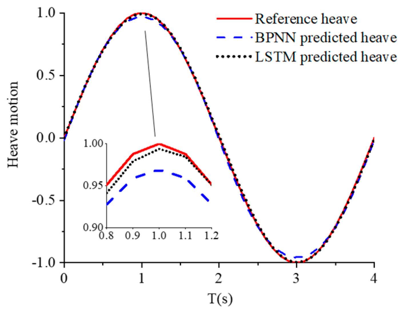
After investigating regular structure motion cases and providing preliminary concluding remarks, the cases of irregular structure motion are examined in this section. The irregular structure motion of an offshore structure is obtained from Kelvin Hydrodynamic Laboratory, University of Strathclyde. The irregular wave power density is distributed as a wave power spectrum. In this paper, the wave power spectrum is a JONSWAP (Joint North Sea Wave Project) spectrum. The irregular waves were composed of more than 50 components. The paper uses experiments to acquire data because there are currently no full-scale ship test conditions available. Firstly, the paper uses the JONSWAP spectrum in model scale to validate the proposed method; the conversion scale ratio between themodel and the full-scale ship is confirmed based on the Froude criterion. Secondly, if put into use to fulfill prediction requirements in real seas, the proposed NN model and system will need to be retrained with full-scale data that involves investigation and recording of real-time motion or wave height. Additionally, if the real seas or the structure model change, the prediction NN model and system will need to be retrained accordingly by means of methods such as incremental training. Thus, the experimental data cannot be used in real seas, whose simulation will be carried out based on the retraining of the prediction NN model with full-scale data. The prediction results of the heave structure motion in irregular waves are shown in Figure 13.
The sampling frequency of the height meter is 100 Hz. The recorded heave motion is curved in the upper subfigure of Figure 14. The reference heave motion is normalized as the regular motion case. The discussion in this section is separated into two parts. The first part determines the optimal feedforward step of the PID control system, and the second part compares the performance of the control system when the two machine learning prediction algorithms are used.
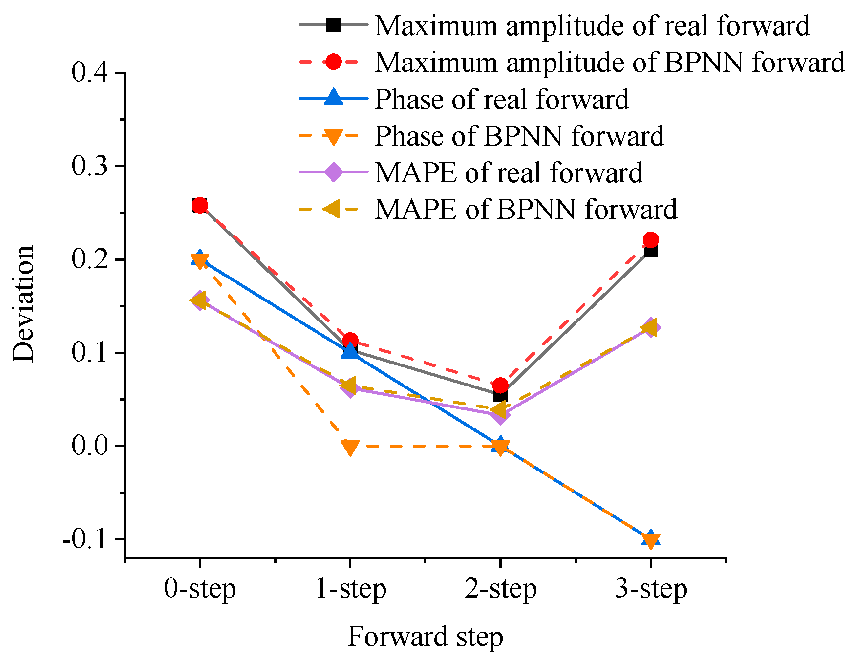
The dominant frequency of structure motion in Figure 14 is approximately 1 Hz. The amplitude of the irregular motion case is 0.028 (Table 6) and that of the regular case with 1 Hz motion frequency is 0.021 (Table 4). Comparison of the performance of the actual-data feedforward cases indicates that the amplitude of the irregular motion case is slightly larger than that of the regular case under the dominant frequency. The compensation effect of irregular motion is approximate to that of the dominant frequency. This result indicates that the capacity of the proposed control method in irregular motion state is as good as that in the regular motion condition. The difference between the two cases may be caused by other components with a high vibration frequency. As shown in Figure 14, the one-step and two-step feedforward control cases perform well. When the number of prediction steps increases to three, the performance worsens again, but it is still a better choice than the feedback control. Between the one-step and two-step cases, the latter is superior because of its smaller motion amplitude of load heave. Therefore, the optimal step number is two when the prediction process is implemented.
In the case of irregular structure heave motion, the BPNN prediction does not meet the accuracy requirement as well as it does in the regular motion cases. The advanced machine learning algorithm, namely, LSTM RNN, is also implemented to predict the future motion in a feasible manner. Two pairs of curves almost overlap in Figure 15. The first pair is the one-step BPNN feedforward case and the case without feedforward (feedback). A possible reason for this overlapping phenomenon is the inaccurate prediction of the BPNN algorithm. Irregular motion is a complex time series variation for BPNN. Therefore, a simple BPNN model is expected to unsuccessfully predict the next step motion, but its result is close to the current step motion. Thus, the curves overlap because they have almost the same input. The second pair is the two-step BPNN feedforward case and the one-step LSTM RNN feedforward case. From another indirect aspect, the LSTM RNN prediction motion is proven accurate.
The overlapped cases mentioned above have similar deviation values regardless of the maximum amplitude, MAE or RMSE. The heave motion of the BPNN prediction cases is much larger than that of the actual-data feedforward control cases, so BPNN is not a recommended prediction algorithm for irregular motions. Heave compensation system control based on LSTM RNN prediction can minimise the motion amplitude with different numbers of prediction steps. Two-step LSTM RNN prediction has the best effect on compensating for the payload motion.

5. Conclusions

To minimise the motion amplitude of payload with an active compensation system, this study proposes a predictive control strategy with prediction algorithms based on machine learning. To verify the proposed predictive control strategy, the reliability of the prediction algorithms is validated, and different algorithms are adopted for regular and irregular wave conditions. The optimal feedforward step of the prediction horizon is determined with different structure motion and sampling frequencies. The influence of the predictive motion on the compensation performance is analysed by comparing such a case with actual-data feedforward cases. The following conclusions are derived:
(1)
For the regular structure motion case, the BPNN algorithm has the advantage of low computational cost. The computational cost of the compensation system with actual-data feedforward control is reduced to 5.5% of the value for reference motion and 6.5% of the value for machine learning predicted motion. Thus, machine learning-based predictive control is reliable for use in active heave compensation systems.
(2)
Comparison of the performance under different sampling and motion frequencies shows that two-step feedforward control is the optimal prediction horizon for the predictive control strategy for the current problem in the paper. The amplitude of payload motion is proportional to the structure motion frequency and inversely proportional to the sampling frequency. The phase deviation is insensitive to the structure motion frequency and sampling frequency.
(3)
In the irregular structure motion case, the LSTM RNN algorithm performs better than BPNN. The amplitude of payload motion is compensated to 2.9% of the reference motion via two-step feedforward control. The compensation effect of irregular motion is approximate to that of the corresponding dominant frequency.
The work focuses on the predictive control strategy of active heave compensation, and it is expected to contribute to motion control for floating structures under realistic conditions. A mechanical actuator will be considered in future research to analyse the practical efficiency of the proposed predictive control strategy.

Author Contributions

Conceptualization, L.H. and M.Z.; methodology, L.H.; software, M.Z.; validation, Z.-M.Y., W.L. and H.Z.; formal analysis, Z.-M.Y.; investigation, W.L.; writing—original draft preparation, M.Z.; writing—review and editing, L.H. All authors have read and agreed to the published version of the manuscript.

Funding

This research was funded by the Natural Science Foundation of Shandong Province (Grant No. ZR2020ME263); the Open Project Program of Shandong Marine Aerospace Equipment Technological Innovation Center, Ludong University (Grant No. MAETIC2021-10); the National Natural Science Foundation of China (51979131, 51509124 and 51681340360); and the China Scholarship Council Foundation (CSC201806680085). The authors extend their sincere gratitude to the abovementioned organizations.

Institutional Review Board Statement

Not applicable.

Informed Consent Statement

Not applicable.

Data Availability Statement

Not applicable.

Acknowledgments

The authors would like to express their sincere gratitude to the support from the Natural Science Foundation of Shandong Province, Ludong University, as well as the National Natural Science Foundation of China. The authors extend their sincere gratitude to the abovementioned organizations.

Conflicts of Interest

The authors declare that they have no known competing financial interest or personal relationship that could have appeared to influence the work reported in this paper. The funders had no role in the design of the study; in the collection, analyses, or interpretation of data; in the writing of the manuscript; or in the decision to publish the results.

References

  1. Ning, X.; Zhao, J.; Xu, J. The heave motion estimation for active heave compensation system in offshore crane. In Proceedings of the 2016 IEEE International Conference on Mechatronics and Automation, Harbin, China, 7–10 August 2016; pp. 1327–1332. [Google Scholar]
  2. Richter, M.; Schaut, S.; Walser, D.; Schneider, K.; Sawodny, O. Experimental validation of an active heave compensation system: Estimation, prediction and control. Control Eng. Pract. 2017, 66, 1–12. [Google Scholar] [CrossRef]
  3. Ren, Z.; Skjetne, R.; Verma, A.; Jiang, Z.; Gao, Z.; Halse, K. Active heave compensation of floating wind turbine installation using a catamaran construction vessel. Mar. Struct. 2021, 75, 102868. [Google Scholar] [CrossRef]
  4. Zhou, H.; Cao, J.; Yao, B.; Lian, L. Hierarchical NMPC–ISMC of active heave motion compensation system for TMS–ROV recovery. Ocean. Eng. 2021, 239, 109834. [Google Scholar] [CrossRef]
  5. Woodacre, J.; Bauer, R.; Irani, R. A review of vertical motion heave compensation systems. Ocean Eng. 2015, 104, 140–154. [Google Scholar] [CrossRef]
  6. Küchler, S.; Mahl, T.; Neupert, J.; Schneider, K.; Sawodny, O. Active control for an offshore crane using prediction of the vessel’s motion. IEEE/ASME Trans. Mechatron. 2010, 16, 297–309. [Google Scholar] [CrossRef]
  7. Neupert, J.; Mahl, T.; Haessig, B.; Sawodny, O.; Schneider, K. A heave compensation approach for offshore cranes. In Proceedings of the 2008 American Control Conference, Seattle, WA, USA, 11–13 June 2008; pp. 538–543. [Google Scholar]
  8. Hatleskog, J.; Dunnigan, M. Heave Compensation Simulation for Non-Contact Operations in Deep Water. In Proceedings of the Heave Compensation Simulation for Non-Contact Operations in Deep Water, Boston, MA, USA, 18–21 September 2006; pp. 1–6. [Google Scholar]
  9. Küchler, S.; Eberharter, J.K.; Langer, K.; Schneider, K.; Sawodny, O. Heave motion estimation of a vessel using acceleration measurements. IFAC Proc. Vol. 2011, 44, 14742–14747. [Google Scholar] [CrossRef] [Green Version]
  10. Huang, X.; Lei, D.; Cai, L.; Tang, T.; Wang, Z. Heave compensation prediction based on echo state network with correntropy induced loss function. PLoS ONE 2019, 14, e0217361. [Google Scholar] [CrossRef] [PubMed]
  11. Shi, B.; Xian, L.; Wu, Q.; Zhang, Y. Active heave compensation prediction research for deep sea homework crane based on KPSO-SVR. In Proceedings of the 33rd Chinese Control Conference, Kunming, China, 22–24 May 2014; pp. 7637–7642. [Google Scholar]
  12. Ngo, Q.H.; Nguyen, N.P.; Nguyen, C.N.; Tran, T.H.; Ha, Q.P. Fuzzy sliding mode control of an offshore container crane. Ocean Eng. 2017, 140, 125–134. [Google Scholar] [CrossRef] [Green Version]
  13. Shi, M.; Guo, S.; Jiang, L.; Huang, Z. Active-Passive Combined Control System in Crane Type for Heave Compensation. IEEE Access. 2019, 7, 159960–159970. [Google Scholar] [CrossRef]
  14. Yang, Y.; Cui, K.; Shi, D.; Mustafa, G.; Wang, J. PID control with PID event triggers: Theoretic analysis and experimental results. Control Eng. Pract. 2022, 128, 105322. [Google Scholar] [CrossRef]
  15. Feng, H.; Sun, W.; Tang, G.; Wang, J. Study on a novel two-part underwater towed system for near-surface towed vehicle test. Ocean Eng. 2022, 255, 111440. [Google Scholar] [CrossRef]
  16. Liu, J.; Wang, L. Two-stage vibration-suppression framework for optimal robust placements design and reliable PID gains design via set-crossing theory and artificial neural network. Reliab. Eng. Syst. Saf. 2023, 230, 108956. [Google Scholar] [CrossRef]
  17. Metzmacher, H.; Syndicus, M.; Warthmann, A.; Treeck, C. Exploratory comparison of control algorithms and machine learning as regulators for a personalized climatization system. Energy Build. 2022, 255, 111653. [Google Scholar] [CrossRef]
  18. Wang, H.; Ding, Z.; Tang, R.; Chen, Y.; Fan, C.; Wang, J. A machine learning-based control strategy for improved performance of HVAC systems in providing large capacity of frequency regulation service. Appl. Energy 2022, 326, 119962. [Google Scholar] [CrossRef]
  19. Han, J. From PID to Active Disturbance Rejection Control. IEEE Trans. Ind. Electron. 2009, 56, 900–906. [Google Scholar] [CrossRef]
  20. Paramesh, S.; Rajendran, S. A unified seakeeping and manoeuvring model with a PID controller for path following of a KVLCC2 tanker in regular waves. Appl. Ocean Res. 2021, 116, 102860. [Google Scholar]
  21. Zeng, Z.; Chen, G. Multi-step Predictions for Generalized Heave Motion of Wave Compensating Platform Based on ELMAN Neural Network. In Proceedings of the 2009 Third International Symposium on Intelligent Information Technology Application Workshops, NanChang, China, 21–22 November 2009; pp. 460–463. [Google Scholar]
  22. Guo, X.; Zhang, X.; Tian, X.; Li, X.; Lu, W. Predicting heave and surge motions of a semi-submersible with neural networks. Appl. Ocean Res. 2021, 112, 102708. [Google Scholar] [CrossRef]
  23. Li, L.; Yuan, Z.; Gao, Y. Maximization of energy absorption for a wave energy converter using the deep machine learning. Energy 2018, 165, 340–349. [Google Scholar] [CrossRef] [Green Version]
  24. Zhao, Q.; Hu, X.; Lin, J.; Deng, X.; Li, H. A novel short-term blood pressure prediction model based on LSTM. AIP Conf. Proc. 2019, 2058, 020003. [Google Scholar]
Figure 1. Sketch of the active heave compensation system for an offshore crane.
Jmse 11 00821 g001
Figure 2. PID predictive control diagram.
Jmse 11 00821 g002
Figure 3. Architecture of BPNN.
Jmse 11 00821 g003
Figure 4. Architecture of the LSTM memory block.
Jmse 11 00821 g004
Figure 5. Controller response motions of a sinusoidal signal based on actual-data feedforward control.
Jmse 11 00821 g005
Figure 6. Heave motion of the payload of a sinusoidal signal based on actual-data feedforward control.
Jmse 11 00821 g006
Figure 7. Prediction results of BPNN and LSTM RNN.
Jmse 11 00821 g007
Figure 8. Controller response motions of a sinusoidal signal based on prediction feedforward control.
Jmse 11 00821 g008
Figure 9. Heave motion of the payload of a sinusoidal signal based on prediction feedforward control.
Jmse 11 00821 g009
Figure 10. Comparison of the deviation between actual-data and prediction feedforward control (sinusoidal signal).
Jmse 11 00821 g010
Figure 11. Amplitudes of payload motion with different numbers of steps.
Jmse 11 00821 g011
Figure 12. Amplitudes of payload motion with different frequencies of structure motions.
Jmse 11 00821 g012
Figure 13. Prediction results of the heave structure motion in irregular waves.
Jmse 11 00821 g013
Figure 14. Heave motions of the payload of irregular structure motion based on actual-data feedforward control.
Jmse 11 00821 g014
Figure 15. Compensated heave motions of the payload of irregular structure motion.
Jmse 11 00821 g015
Table 1. Comparison of deviations based on actual data and prediction.
Types of FeedforwardTypes of Deviation
Maximum AmplitudePhase/StepMAERMSE
Without forward0.25820.1560.175
One-step actual-data feedforward0.10310.0620.070
Two-step actual-data feedforward0.05500.0330.038
Three-step actual-data feedforward0.210−10.1270.143
One-step BPNN prediction0.11300.0650.072
Two-step BPNN prediction0.06500.0390.043
Three-step BPNN prediction0.221−10.1270.143
Table 2. Amplitude deviation with different numbers of prediction steps ( ω s = 10 Hz).
Motion Frequency (Hz)0.06250.1250.250.51
Forward step00.0650.1300.2580.4950.866
10.0260.0520.1030.1980.346
20.0130.0270.0550.1230.319
30.0520.1050.2100.4200.848
40.0920.1830.3630.7061.277
50.1310.2610.5160.9851.663
Table 3. Phase deviation with different numbers of prediction steps ( ω s = 10 Hz).
Motion Frequency (Hz)0.06250.1250.250.51
Forward step022122
111111
20000−1
3−1−1−1−1−2
4−2−2−1−2−3
5−3−3−2−3−4
Table 4. Amplitude deviation with different numbers of prediction steps ( ω s = 100 Hz).
Motion Frequency (Hz)0.06250.1250.250.51
Forward step00.0070.0130.0260.0520.105
10.0030.0050.0110.0210.042
20.0010.0030.0050.0110.021
30.0050.0110.0210.0420.084
40.0090.0180.0370.0730.146
50.0130.0260.0520.1050.209
Table 5. Phase deviation with different numbers of prediction steps ( ω s = 100 Hz).
Motion Frequency (Hz)0.06250.1250.250.51
Forward step022222
111111
200000
3−1−1−1−1−1
4−2−2−2−2−2
5−3−3−3−3−3
Table 6. Comparison of the deviation of different prediction algorithms.
Types of FeedforwardTypes of Deviation
Maximum AmplitudeMAERMSE
Without forward0.1200.0230.030
One-step actual-data feedforward0.0480.0080.010
Two-step actual-data feedforward0.0280.0040.006
One-step BPNN prediction0.1220.0230.030
Two-step BPNN prediction0.0690.0100.013
One-step LSTM prediction0.0600.0100.013
Two-step LSTM prediction0.0290.0050.006
Disclaimer/Publisher’s Note: The statements, opinions and data contained in all publications are solely those of the individual author(s) and contributor(s) and not of MDPI and/or the editor(s). MDPI and/or the editor(s) disclaim responsibility for any injury to people or property resulting from any ideas, methods, instructions or products referred to in the content.

