A Contrastive-Learning-Based Method for the Few-Shot Identification of Ship-Radiated Noises

Abstract

For identifying each vessel from ship-radiated noises with only a very limited number of data samples available, an approach based on the contrastive learning was proposed. The input was sample pairs in the training, and the parameters of the models were optimized by maximizing the similarity of sample pairs from the same vessel and minimizing that from different vessels. In practical inference, the method calculated the distance between the features of testing samples and those of registration templates and assigned the testing sample into the closest templates for it to achieve the parameter-free classification. Experimental results on different sea-trial data demonstrated the advantages of the proposed method. On the five-ship identification task based on the open-source data, the proposed method achieved an accuracy of $0.68$ when only five samples per vessel were available, that was significantly higher than conventional solutions with accuracies of $0.26$ and $0.48$. Furthermore, the convergence of the method and the behavior of its performance with increasing data samples available for the training were discussed empirically.

1. Introduction

Classifying vessels of interest from the received ship-radiated noises is a key task in underwater acoustical signal processing [1,2,3]. Many approaches have been proposed for it, some of them focused on the physical feature extraction from the noise [2,4,5], while in recent years, others tried to deal with it in the data-driven manner with the help of popular deep learning methods [6,7,8,9]. After optimizing the parameters of the models on the training set, deep-learning-like methods automatically extracted abstract features beneficial to the final task from the raw signal waveform or time-frequency spectrogram. And massive impressive improvements on the testing set can be achieved by such trained models compared to conventional feature extraction approaches [3,10].

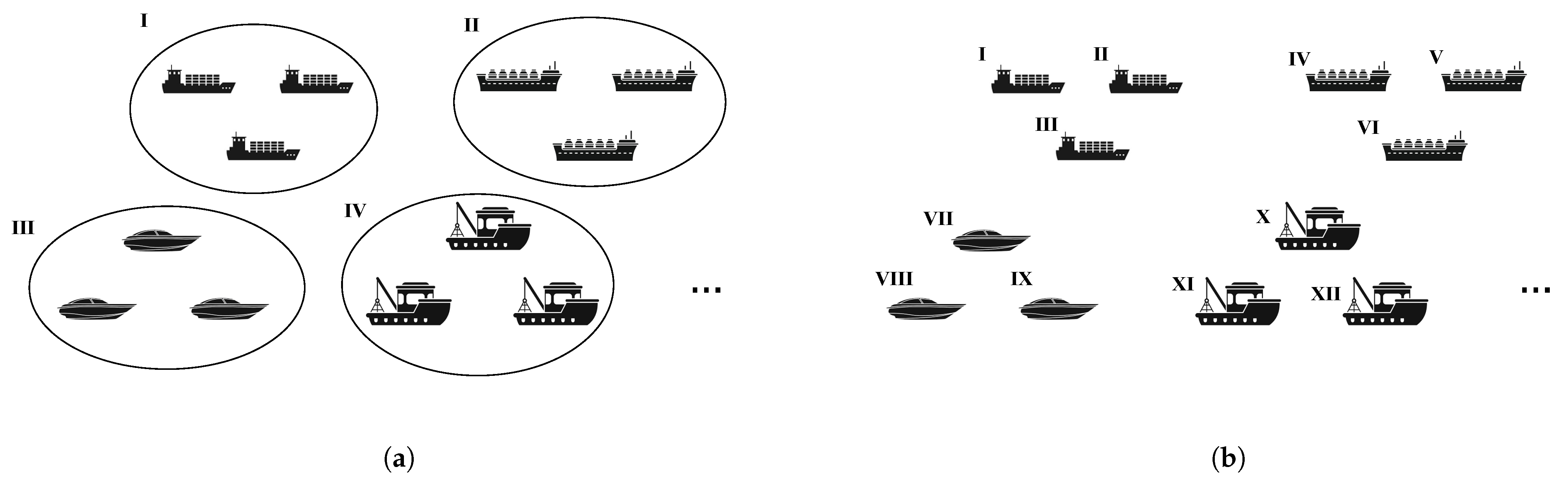
In current research, it was common practice to first assign involved vessels into several coarse categories artificially based on a certain attribute (such as the purpose of the vessel), and then, the effective methods were expected to automatically and accurately classify underlying vessels to one of the above categories (e.g., cargo ships, tankers, etc.) according to the received ship-radiated noise. The decision foundations for an automatic method were the differences in the physical or statistical characteristics of radiated noises, which came from the differences in the engines carried and the hull structure itself. But the division of ship-categories was usually based on practical attributes (such as the purpose as mentioned above). The potential inconsistency between the two led to the large variances between different individual vessels within the same category. For example, the assigned cargo ships category might include original cargo ships and those converted from passenger ships, whose radiated noises were obviously different. Thus, it could be considered that there was the large intra-class variances problem in the classification of ship-radiated noises [11,12]. A possible solution to this issue is to divide the categories in a fine-grained manner that could decrease the intra-class variances. Based on the received ship-radiated noises, the task of identifying the individual IDs of vessels (named as ship identification) rather than classifying into the coarse categories (named as ship classification) was therefore considered in this work. The task of this type might be interesting for some practical applications as well, such as area maritime security, harbor verification for entry and departure of vessels, etc. [13]. However, to the best of our knowledge, the existing literature has paid less attention to this task.

Ship identification could be understood as a fine-grained setting of the conventional classification, but the fine-grained categories bring not only the conceptual extensions but also some non-trivial changes into the ship identification setting. Obviously, the outputs of methods for the identification problem would be in a higher-dimensional state space because the number of vessel individuals is much greater than that of vessel categories. It increases the difficulty of the task and intensifies the data-hungriness of deep-learning-like algorithms. However, it is difficult to obtain numerous real-world ship-radiated noises from different targets, which has made classification tasks for ship-radiated noises suffer from data scarcity, and such a scenario was called few-shot classification in existing works [10,14,15]. The property of data scarcity is exacerbated by the fine-grained nature of the ship identification problem since the increase of categories greatly dilutes the amount of data in each category. Each vessel may only contain a few minutes or less of real-world data (e.g., 2 min for each vessel), which means that only a few spectrograms may be available after time-frequency analysis. Many existing studies in the classification task of ship-radiated noise tried to cope with the limitation of the real-world data scarcity by redesigning the network architecture. The attention mechanism was employed in [16] to get the relationship between different low-frequency line spectra of the ship-radiated noise; the recurrent-wavelet auto-encoder architecture was proposed in [17] to deal with the effect of time-varying marine environments while extracting the periodic frequency components of the ship-radiated noise; and [18] considered a spectrogram transformer model to obtain the global information of the time-frequency spectrogram automatically. Beyond the architectural design, reducing the need of real-world data for deep neural networks in ship classification tasks by improving learning strategies has also attracted much attention. [19] argued that the unsupervised pre-training can enable the deep long short-term memory network to effectively address the lack of data; by augmenting the 3D mel-spectrogram of ship-radiated noise in the time and frequency domains [20], it was believed that the classification performance can be improved with limited real-world data; and [21] considered that the performance of ship classification tasks would benefit from the ensemble of conventional SoftMax loss and metric-based loss when optimizing the models. However, the available training samples in existing works on classification of ship-radiated noises were still more than hours even with limited real-world data, and the situation of only a few available samples (e.g., <10 spectrograms for each vessel) that might be faced in ship identification has not been fully discussed.

Moreover, since ship identification methods need to distinguish each individual of vessels, a certain class (individual) of samples in the training set for methods could be considered as templates for the individual in other soundscapes. This situation is also different from conventional ship classification. The potential benefit of available individual registration templates is less considered in the ship classification problem.

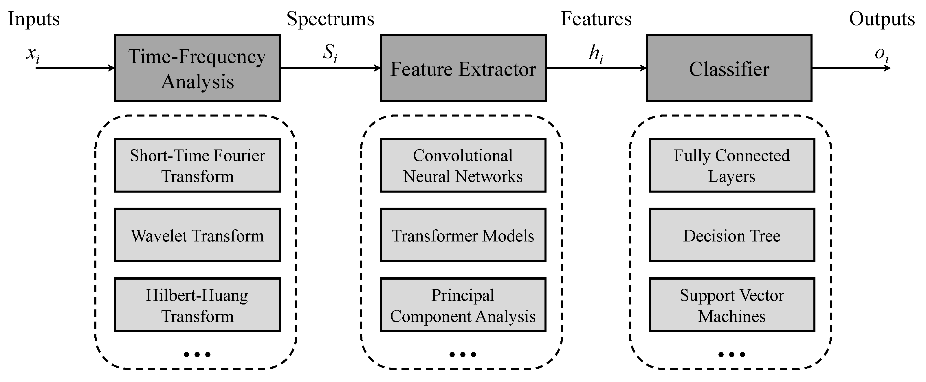
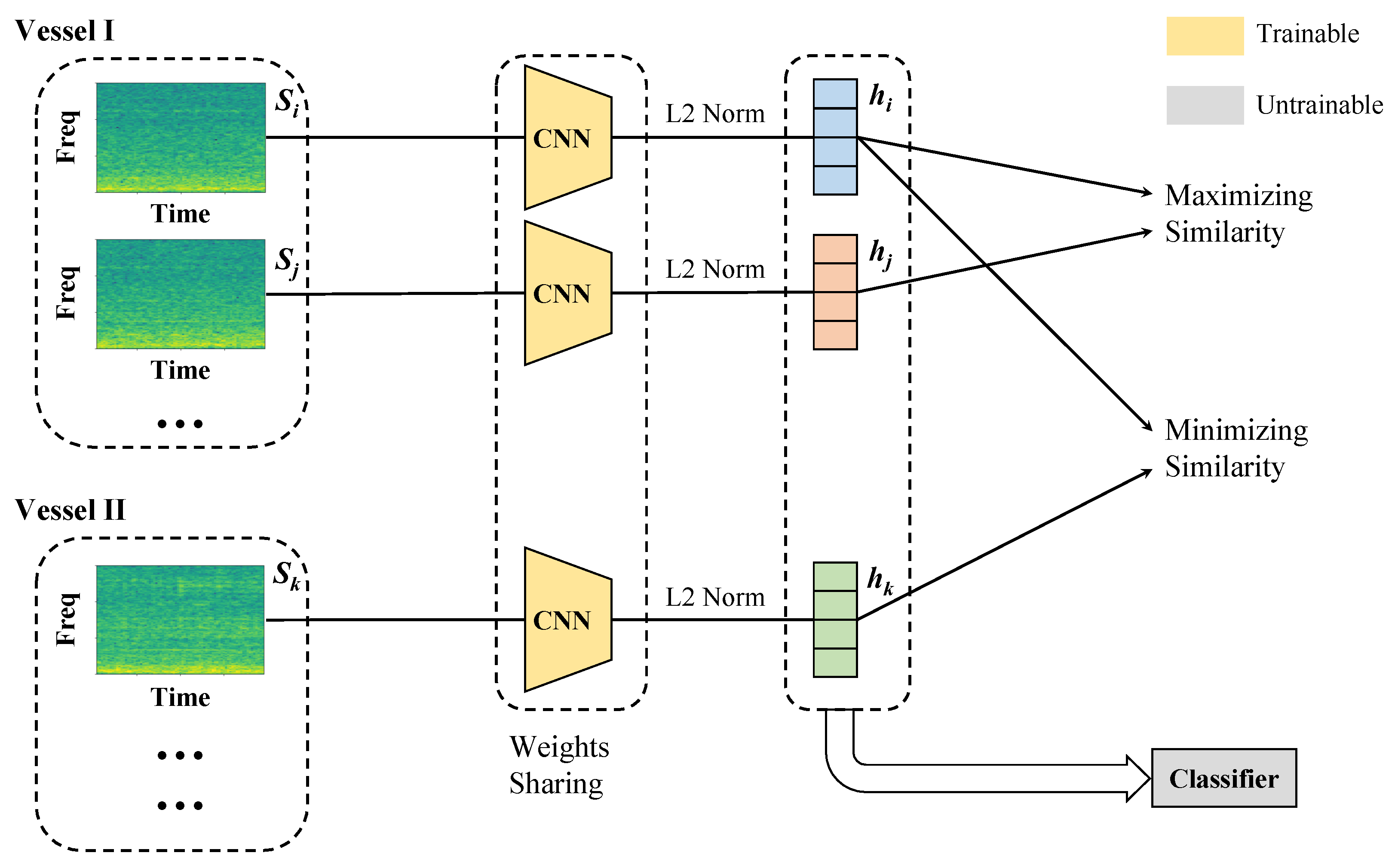
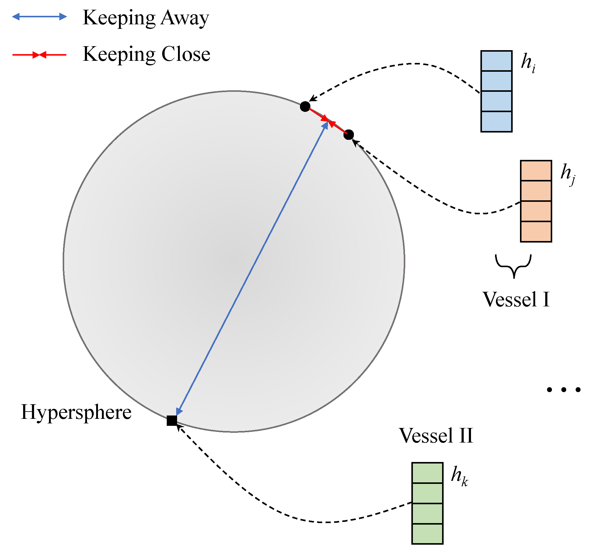
We proposed a contrastive-learning-based method to adapt the few-shot ship identification problem. It did not contain a parameterized classifier, and only employed the convolutional neural networks (CNN) as the feature extractor to map the time-frequency spectrogram into the abstract feature space. In the training phase, the proposed method constructed sample-pairs consisting of real-world samples, where the sample-pairs from the same individual’s samples were called as positive pairs, while those from different individuals’ samples were as negative pairs. And the optimization goal was to make the features of positive pairs close, while making those of negative pairs far away, instead of bringing the classifier output of a sample closer to its label. In the testing phase, it treated the training samples as registration templates for each individual, and achieved parameter-free classification by calculating the distance between the testing samples and all templates and selecting the closest one as the discrimination result. The main contributions of this paper are as follows,

• The contrastive-learning-based method was proposed for real-world few-shot ship identification from the received noises. It optimized the parameters of the feature extractor by making positive pairs close and negative pairs far away.
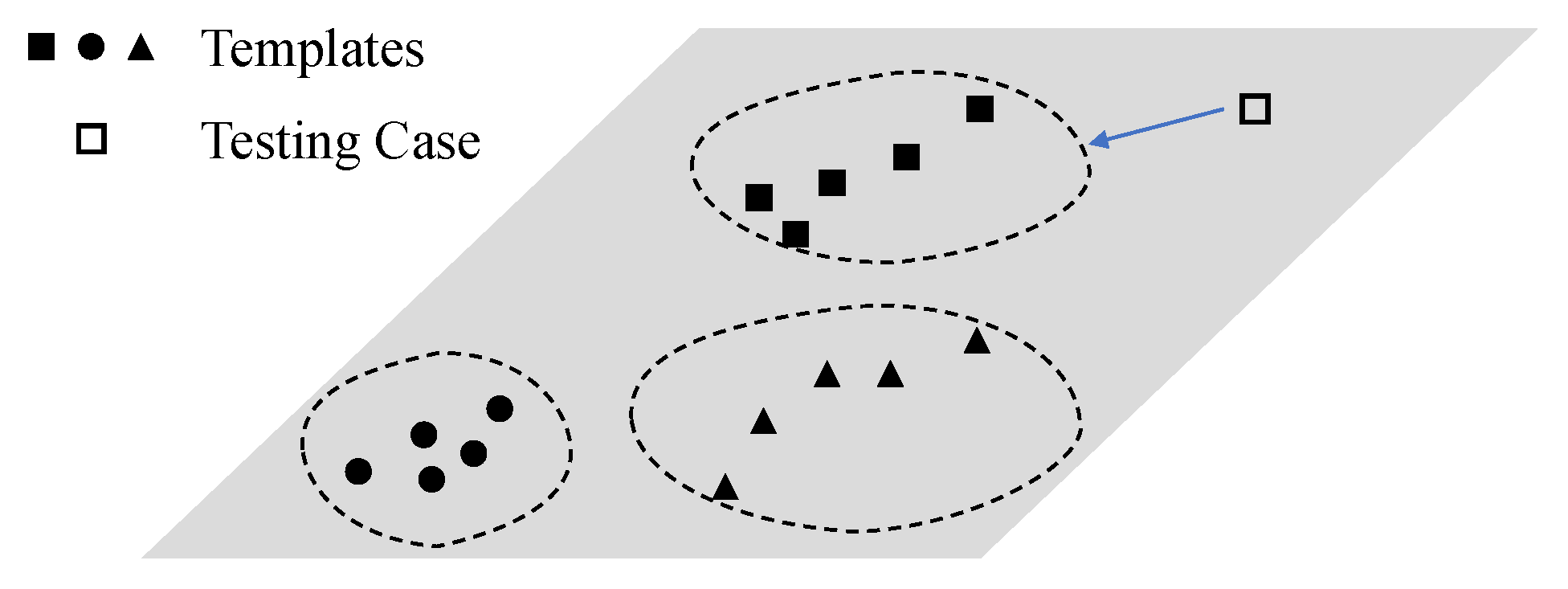
• The available samples were utilized as templates for comparison in addition to serving as the training set. The parameter-free classifier was achieved by choosing the closest distance between the testing samples and all templates in the feature space.
• The performance of the proposed method was verified on the sea-trial datasets, and the role of the number of available samples was also discussed. The results confirmed the advantages of our method in solving the few-shot ship identification problem.

2. Ship Identification from Recorded Noises

In this section, we formalized the ship identification task and illustrated how it differs from the conventional ship classification problem. Furthermore, the general framework of methods for solving classification or identification problems was also described here.

2.1. Problem Definition

Vessels radiated unavoidable noises during the sailing because of the activity of engines, propellers and other components, and differences in hull and mechanical components of each vessel brought the noises vary greatly in the time-frequency domain and auditory perception [22,23]. The differences in ship-radiated noises allowed us to classify them by analyzing the received copies when assuming that there was no serious impairment brought by the propagation in marine environments. The different divisions for categories in classification led to different settings of conventional ship classification and ship identification discussed in this work (Figure 1). In the ship classification task, vessels were usually divided into different categories according to a certain attribute such as their purpose. But different individuals within the same category might vary widely in hull sizes and mechanical parts carried, so there were significant intra-class variances in the ship classification task [24]. If assuming that each individual ship was a category, then the settings for the ship identification task here could be derived, which can play a role in many practices such as area monitoring or maritime anti-smuggling.

Classes of ship identification were with more fine-grained compared with the ship classification, which made the problem of limited availability of real-world samples for each class in ship classification even more severe in ship identification. The realistic data available for each individual vessel might only be a few minutes or less. To formalize such a scenario, we introduced the N-way K-shot setting commonly employed in few-shot learning [25,26], which assumed that there were N classes and each class contained K samples (usually, $K\le 10$). The received noises available for training were with the continuous time axis, and it was a routine to split the training data into frames [3,27], so the above K referred to the number of these short frames (e.g., if the available training data for each class lasted 1 min and was split into 2-s frames without overlapping, then K here was 30). Additionally, the number of classes in the ship identification (i.e., N) was usually much larger than that in the ship classification (Figure 1) because finer distinctions were needed, which increased the difficulty of the identification task. But there were also a potential benefit because small intra-class variances brought by the finer classes made samples available in the training could be employed as registration templates for the comparison in the testing, and gains might be obtained by considering this.

Therefore, for the ship identification tasks under the N-way K-shot setting, the known information is that there are N vessels and K frames of data for each of the vessels could be provided. When another utterance of noise received in different soundscapes (or the source vessel sails under different working conditions) is given, and the utterance is confirmed a priori to come from the above N vessels, methods can be considered to work well if they can utilize the known information to automatically and accurately identify which vessel the utterance comes from.

2.2. General Framework of Methods

For the tasks of classifying ship-radiated noises automatically, the solutions mostly followed the pipeline in Figure 2. After framing the received noise of long duration, methods were fed with the short frames $x_i$. Their spectrums $S_i$ were obtained by the preprocessing of time-frequency analysis technologies. Deep neural networks such as CNN [28] or feature extraction algorithms in classic machine learning such as principal component analysis (PCA) [29] exploited information in the temporal and frequency dimensions for feature modeling, and mapped spectrums $S_i$ to features $h_i$. This part was called the feature extractor, which discarded the redundant information in the data for dimensional compression. Finally, the classifier transformed features $h_i$ into the class vectors $o_i$, whose dimensionality depended on the tasks themselves (it would be N under the N-way K-shot settings). The class vectors $o_i$, although not well-calibrated [30], could be interpreted as approximations to class-conditional probability distributions [31]. With the help of the maximum a posteriori criterion [31], the prediction results for the category or ID of vessels corresponding to the inputs $x_i$ (short frames of the received noises) could be returned.

Modern deep learning methods typically employed parameterized feature extractors and classifiers in the pipeline. Their parameters needed to be optimized so that methods can return the expected outputs in practice. Therefore, a portion of the data was taken out separately to train the models. A common optimization objective in conventional classification problems was to minimize the cross-entropy losses between the predicted class vectors $o_i$ and the corresponding labels $y_i$ of the data [29]. With the help of gradient backpropagation [32] and stochastic-gradient-descent-like algorithms (such as Adam optimizer [33]), the parameters of the models were updated epoch by epoch to try to gradually reduce the losses. After the parameters were optimized, the models were required to make predictions on another portion of the real-world data and compare them with the labels to evaluate the final performance of methods. It was worth noting that for ship classification or identification tasks, the real-world data adopted for evaluation should be with the different soundscapes than that adopted to optimize the models to ensure that the generalization was examined instead of overfitting [9]. These two parts could be from the same vessel sailing at significantly different time-periods (or positions) or under different working conditions.

3. Proposed Methods

In this section, the paradigm of the proposed contrastive-learning-based methods were first demonstrated. Next, the mechanism of the feature extractor, maximization and minimization of similarity, and the classifier were described separately. Finally, the practical training flow of the proposed approaches under the N-way K-shot settings were detailed.

3.1. Proposed Contrastive-Learning-Based Methods

The schematic diagram of our few-shot ship identification methods based on contrastive learning was shown in Figure 3. Unlike the conventional ship classification methods introduced in Section 2.2, our strategy of optimizing the parameters of the feature extractors (CNN employed in this work) was not to minimize the distance between the predicted outputs of the classifiers on the data and the labels of the data, but to make the features outputted from the CNN close for the positive pairs (from the same vessel) and distant for the negative pairs (from different vessels). In addition, the parameter-free classifier by comparing the distance in the embedding space between the features of samples to be tested and those of available templates was achieved in the inference phase. Compared with the conventional solutions, the proposed methods increased the cases available for the learning phase from $N·K$ to $\left(\genfrac{}{}{0pt}{}{N·K}{2}\right)$ in the scenario of few-shot ship identification. The fully-connected (FC) layers were avoided in the classifier, which contained huge parameter overhead and were highly susceptible to overfitting when the amount of training samples was insufficient [34].

After the received noise utterances available for the training were split into short frames $x_i$ with the length of 2 s, the time-frequency representations $S_i$ of these frames $x_i$ were obtained by short-time Fourier transform (STFT), in which the STFT employed a Hamming window with a length of 100 ms and a hopping length of 25 ms. The features in the embedding space $h_i$ were generated after these representations $S_i$ were sequentially passed through the weight-shared CNN and the L2 normalization operator. Assuming that the CNN with trainable parameters $\theta$ was ${\mathcal{F}}_{\theta }(·)$,

$$h_i=\parallel {\mathcal{F}}_{\theta }(S_i)\parallel ,$$

(1)

where $\parallel ·\parallel$ represented the L2 normalization.

If the similarity measure $\mathcal{M}(·,·)$ was chosen, the optimization objective in the training phase was as

$$\underset{\theta }{max}\mathcal{M}(h_i,h_j),$$

(2)

when i and j were different indexes of the same vessel; and as

$$\underset{\theta }{min}\mathcal{M}(h_i,h_k),$$

(3)

when i and k were from different vessels.

During the practical inference, if the trained parameters of the CNN were $\widehat{\theta }$ and the spectrogram of the sample to be tested was $\tilde{S}$, then the corresponding ship ID identified by the methods was as

$$\underset{v}{\mathrm{argmax}}\sum _{i\in {\Phi }_v}\mathcal{M}(\parallel {\mathcal{F}}_{\widehat{\theta }}(S_i)\parallel ,\parallel {\mathcal{F}}_{\widehat{\theta }}(\tilde{S})\parallel ),$$

(4)

where ${\Phi }_v$ was the set of indexes from the same ship ID of v. Under the N-way K-shot settings, there were N sets, and different K indexes in a set. It could be seen from Equation (4) that outputs of our method for the ship identification task depended on the architecture of the feature extractor $\mathcal{F}$, the similarity criterion $\mathcal{M}$ and the optimization of parameters $\theta$ in $\mathcal{F}$.

3.2. CNN Architecture

The popular ResNet-18 architecture [35] was employed in this work as the feature extractor $\mathcal{F}$ and its details were shown in Figure 4. Its basic components were convolutional layers and residual connections. For each convolutional layer, the 2D convolutional operator, the batch normalization and the nonlinear activation function (Rectified Linear Unit, ReLU) were sequentially placed. Parameters to be optimized were mainly contained in the 2D convolutional operators of each layer. In the forward calculation of the CNN used, the time-frequency representations $S_i$ of short frames from received noises first passed through the first convolutional layer and then sequentially through four modules containing residual connections, where the kernel size of the first convolutional layer was $7\times 7$ and that of the convolutional layers involved in those residual modules was $3\times 3$. In the residual modules, the input could optionally skip the next two convolutional layers and connect directly to the output after two layers, which helped prevent the degradation of deep neural networks [35]. During the layer-by-layer processing of the CNN, the channel numbers of data gradually increased while its own size was gradually decreasing, and the size for each channel was reduced to 1 by the final average pooling. Thus, when the time-frequency representations $S_i$ were input, the above CNN returned the 512-dimensional vectors, and these vectors were then normalized (following Equation (1)) to be the features $h_i$ adopted for the downstream identification tasks. With such the layer-by-layer nested parametric models, the raw representations $S_i$ were de-redundant and mapped to a low-dimensional feature space (the dimensionality here was 512). The following similarity calculation and identification were considered in the feature space constructed in this way.

3.3. Maximization and Minimization of Similarity

In our contrastive-learning-based methods, the parameters $\theta$ of the feature extractor $\mathcal{F}$ needed to be optimized on the training set for accurate inference in practice. The optimization objective was to make the features $h_i$ from the same ship ID close to each other on the hypersphere of the abstract feature space, while making those from different ship IDs away from each other (Figure 5). Driven by the objective, the feature extractor was aspired to return features that were more separable in the feature space, and after the optimization, these features could even be distinguished by a simple linear classifier [36]. The property was desirable for the few-shot ship identification, since there was no more data available for training the classifier in our task.

To measure the similarity between two features (512-dimensional vectors), the cosine similarity was employed, which could be expressed as

$$\mathcal{M}(h_i,h_j)=\frac{h_i^T·h_j}{\parallel h_i\parallel ·\parallel h_j\parallel },$$

(5)

where $\mathcal{M}(h_i,h_j)$ was normalized, and ranged from $-1$ to 1.

According to Equations (2) and (3), the multi-objective optimization was involved in the methods. For ease of solving it numerically in the framework of gradient backpropagation, the maximization and minimization of similarity were re-written into the minimization of a single loss via the InfoNCE loss [37]. This loss L could be denoted as

$$L=-\frac{1}{B}\sum _{i=1}^{B}log\frac{{\sum }_{j=1}^B𝟙[j\ne i\&j\in {\Phi }^i]exp(\mathcal{M}(h_i,h_j)/\tau )}{{\sum }_{j=1}^B𝟙[j\ne i]exp(\mathcal{M}(h_i,h_j)/\tau )},$$

(6)

where B was the size of a mini-batch, $𝟙\left[condition\right]$ was the indicator function that equaled 1 when $condition$ held and 0 otherwise, and ${\Phi }^i$ was the set of indexes with the same ship ID as the index i. In addition, $\tau$ was a hyperparameter that was responsible for scaling the similarity (ranging from 0 to 1).

For analyzing the behavior of the loss, L could be re-written as the mean of the contrastive losses $l(i)$ at each anchor i, i.e., $L=\frac{1}{B}{\sum }_{i=1}^{B}l(i)$ with

$$l(i)=log\frac{{\sum }_{j=1}^B𝟙[j\ne i]exp(\mathcal{M}(h_i,h_j)/\tau )}{{\sum }_{j=1}^B𝟙[j\ne i\&j\in {\Phi }^i]exp(\mathcal{M}(h_i,h_j)/\tau )}.$$

(7)

For $l(i)$, it could be interpreted as the ratio of the sum of the similarities of all positive and negative pairs for the anchor i in a mini-batch to the sum of the similarities of positive pairs for the anchor i there. $B-1$ positive and negative pairs would be constructed for the anchor i in a mini-batch, so the numerator of the above ratio was the sum of $B-1$ items, and the denominator was the sum of $B-1-B_n$ items if there were $B_n$ negative pairs in the mini-batch. During the optimization, the decreasing loss meant that in a mini-batch, the sum of similarities of positive pairs was increasing compared to those of negative pairs. This was exactly what was expected in Figure 5.

When $\tau$ approached 0,

$$\begin{array}{cc}\hfill \underset{\tau \to 0^{+}}{lim}l(i)& =\underset{\tau \to 0^{+}}{lim}log(1+\frac{{\sum }_{j=1}^B𝟙[j\notin {\Phi }_i]exp(\mathcal{M}(h_i,h_j)/\tau )}{{\sum }_{j=1}^B𝟙[j\ne i\&j\in {\Phi }^i]exp(\mathcal{M}(h_i,h_j)/\tau )})\hfill \\ \hfill & =\underset{\tau \to 0^{+}}{lim}log(1+exp(\frac{1}{\tau }·(\underset{j\notin {\Phi }_i}{max}\mathcal{M}(h_i,h_j)-\underset{j\ne i\&j\in {\Phi }^i}{max}\mathcal{M}(h_i,h_j)))),\hfill \end{array}$$

(8)

let the maximum similarity in the positive pairs $ma{x}_{j\ne i\&j\in {\Phi }^i}\mathcal{M}(h_i,h_j)$ be ${\mathcal{M}}_p$ and the maximum one in the negative pairs $ma{x}_{j\notin {\Phi }_i}\mathcal{M}(h_i,h_j)$ be ${\mathcal{M}}_n$, and then,

$$\underset{\tau \to 0^{+}}{lim}l(i)=\underset{\tau \to 0^{+}}{lim}log(1+exp(\frac{1}{\tau }·({\mathcal{M}}_n-{\mathcal{M}}_p)))=\underset{\tau \to 0^{+}}{lim}\frac{1}{\tau }max({\mathcal{M}}_n-{\mathcal{M}}_p,0).$$

(9)

From Equation (9), it could be found that when $\tau$ was set small, the loss tended to only focus on the negative pairs if there was an indistinguishable negative pairs (meaning that ${\mathcal{M}}_n$ was even larger than ${\mathcal{M}}_p$). Because there were possible labeling errors, and the feature extractor has not yet converged in the early epochs of training, such indistinguishable negative pairs were almost guaranteed to exist, which in turn led to difficulty in converging or poor generalization [38]. Furthermore, the loss in the perfect convergence $l_c$ (the similarities were 1 for all positive pairs and −1 for negative ones) was equal to $log(1+\frac{B_n}{(B-1-B_n)}·exp(-2/\tau ))$, and that in the perfect misclassification $l_m$ (the opposite situation) was equal to $log(1+\frac{B_n}{(B-1-B_n)}·exp(2/\tau ))$ from Equation (7). It showed that larger $\tau$ made it troublesome for the model to distinguish between positive pairs and negative pairs, and the small gap available for the convergence (from $l_m$ to $l_c$) led to the difficulty for the methods to update the parameters $\theta$. Therefore, it could be considered that the role of the hyperparameter $\tau$ in Equation (6) was to control the attention of models to the negative pairs; and when $\tau$ was reduced from 1 to 0, the models tended to focus more on the hard negative pairs. The hyperparameter $\tau$ was $0.2$ in follow-up experiments if not specified.

3.4. Distance-Based Classifier

Typically, classifiers were implemented with FC layers [29]. But FC layers contained numerous parameters and were prone to overfitting [34]. As a result, it was difficult to train a classifier composed of FC layers with good performance under our few-shot ship identification task. Fortunately, as our optimization objective showed (Figure 5 and Equation (6)), after the training, the outputs of the feature extractor were similar for vessels with the same ID, and dissimilar from each other for those with different IDs. So the distance-based classification for the outputs of the feature extractor could be considered (Figure 6).

The expression of such a classifier was shown in Equation (4). During the inference, it treated all samples in the training set as registration templates; the well-trained feature extractor applied the forward calculation on these templates and the samples to be tested, and compared the similarities between them in the feature space defined by the trained model. Samples to be tested were finally assigned into the ship ID of the registration templates with the greatest sum of similarities. The distance-based classifier was like to the k-nearest neighbors (KNN) classifier, but it did not require a given hyperparameter k a priori as in KNN.

3.5. Training for the Proposed Methods

For contrastive-learning-like methods, the key to making them work was to prevent the feature extractors from falling into a collapse solution, where the models mapped all inputs to near the same point on the hypersphere of the feature space [39]. The role of the negative pairs in the InfoNCE loss function (Equation (6)) was to prevent the feature extractors from collapse, and enough negative pairs helped the models stay away from the collapse solution [36]. In our work with the N-way K-shot setting, $NK-1$ sample-pairs could be constructed for each anchor sample, of which there were $K-1$ positive pairs and $(N-1)K$ negative pairs. During the training, we filled a batch with all positive and negative pairs of an anchor sample. The batch size was thus $NK-1$, and a batch contained $(N-1)K$ negative pairs. For example, if the three-ship identification was concerned and there were five real-world samples available for each vessel (i.e., $N=3$ and $K=5$), the total number of samples for developing models would be 15. The number of sample-pairs constructed for each sample in the method was 14, including 4 positive pairs and 10 negative pairs. During a full training epoch, the construction on sample-pairs was applied for each sample and sample-pairs corresponding to a sample were put into a batch, so there are 15 batches and a total of 210 sample-pairs involved in an epoch for the case.

Since the values of N and K in our task were usually not large, the proportion of negative pairs in a batch cannot completely prevent the feature extractors from converging to a collapse solution during the optimization. Beyond the utilization of negative pairs, stopping gradient flow was also beneficial to prevent the model collapse during the update of parameters in the optimization [40]. The trick was also implemented in the training pipeline of our methods. When it computed the gradient of the loss for the backpropagation, all but the anchor sample were stripped from the computational graph. It meant that for the weight-shared CNN, only the partial derivative of the loss to the weights of the CNN at the anchor sample was computed; and then, the backpropagation was applied by calculating the gradient with this partial derivative; and finally, the weights of the CNN were updated. Because all samples acted as the anchor sample by turns in different mini-batches of an epoch of the training, the optimization problem of fixing one and solving the other was computed alternately in an epoch, which facilitated the models to stay away from the collapse solution.

The pseudocode of the parameter update for neural networks in the proposed method was described in Algorithm 1, which encapsulated the major details of the training strategy.

Algorithm 1: The training algorithm of neural networks in the proposed method.

4. Experiments, Results and Discussion

In this section, we verified and discussed the performance of the proposed methods for the ship identification task via the sea-trial datasets. Firstly, the sea-trial datasets and settings of identification tasks were presented, and the implementation of the methods was detailed; the advantages of the proposed methods were then revealed by comparing with the baselines under different identification settings; and finally, the target-wise performance, the convergence of the methods and the role on performance of the number of samples available in training were analyzed by empirical studies.

4.1. Sea-Trial Experiments and Datasets

There were two publicly accessible datasets, ShipsEar [41] and DeepShip [42], in the ship classification tasks. DeepShip dataset did not disclose the auxiliary information about the vessels in addition to the data itself and labels on categories. Hence, the dataset cannot be used for our ship identification tasks because it was not possible to know the details about ship IDs of the same category of data. For the ShipsEar dataset, we constructed a ship identification dataset, SID1, based on the provided information on vessels and receiving time of the hydrophone. The selected data IDs [41] were shown in

Table 1. Data IDs employed in the training and testing in SID1, which was built based on ShipsEar.

Vessels	Categories	Data for Training	Data for Testing 1
i	Passenger Boats	ID-7	ID-62
ii	Passenger Boats	ID-9	ID-63
iii	Passenger Boats	ID-11	ID-65
iv	Passenger Boats	ID-14	ID-67
v	Passenger Boats	ID-17	ID-59

¹ Since the lengths of these utterances in the testing set varied, the first 160 s of them were uniformly intercepted for the evaluation.

, and they were all from the passenger boats. Thus, methods developed on the SID1 needed to identify five different passenger boats. Each selected vessel included at least two utterances with the significant separation in the receiving time (more than four hours apart), one of which was employed for training and the others for testing. Its purpose was to expose the training and testing samples in significantly different soundscapes, in order that the obtained results during the testing were exactly related to the generalization of the methods instead of the overfitting.

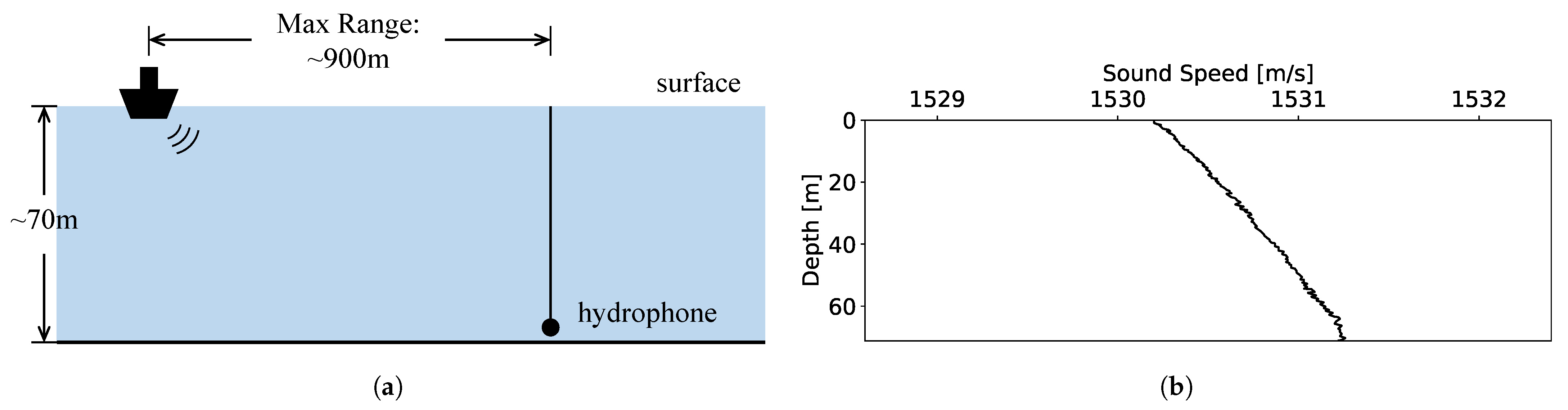
Beyond the open-source datasets, sea trials were carried out in the northern South China Sea during 2022 (Figure 7), in which the hydrophone received the radiated noises from vessels passing in its vicinity (with the sampling rate of 5000 Hz), and the average ocean depth of the experimental area was about 70 m. The corresponding ship IDs were confirmed by the automatic identification system (AIS). For avoiding the potential interference, an utterance of received noise was considered as the effective utterance when the source vessel was within $0.5$ nautical miles near the hydrophone and there were no other oceanic vehicles within 2 nautical miles during this period. In addition, as in the construction of SID1, the selected vessels were required to have more than two temporal-separated effective utterances for splitting the training and testing sets. 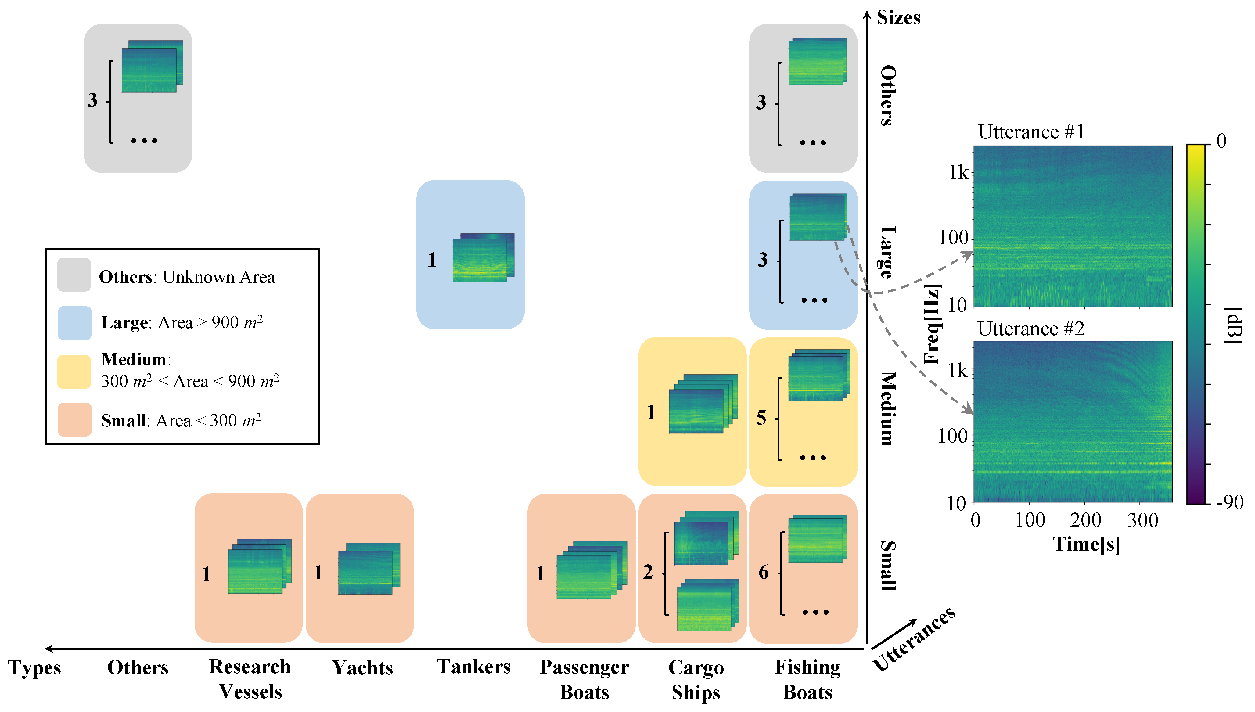With the filtering of the above two conditions, the real-world data on radiated noises was obtained, and it was called as VOS (Vessel Observation by Single-hydrophone) data. There were 27 different individual vessels with a total of 67 utterances of the uniform length of 6 min. These vessels fell into 6 known categories based on the purpose; and they were assigned into 3 types according to their sizes, where vessels with the area (a product of length and width) greater than 900 m${}^2$ were defined as large vessels, those smaller than 300 m${}^2$ were defined as small vessels and the rest were medium vessels. Examples of the time-frequency spectrums and other details on VOS data could be found in Figure 8.

Two datasets, SID2 and SID3, were established for the ship identification tasks based on the above VOS data (

Table 2. Description of three datasets, SID1, SID2 and SID3, for the ship identification tasks.

Dataset	Description
SID1	5 different passenger boats from the ShipsEar dataset
SID2	3 different fishing boats (with sizes of large/medium/small) from the VOS data
SID3	27 different vessels from the VOS data

). Three individual fishing boats with different sizes (large, medium and small) were selected to form SID2, and all available vessels were selected to form SID3. This meant that the methods developed on SID2 were asked to identify 3 different fishing boats, whereas those developed on SID3 had to identify 27 different targets. Obviously, SID3 was more difficult than other counterparts. Under the N-way K-shot setting, the number of vessels here was the value of N, and for emphasizing the property of few-shot scenarios, K was set to 5 in this work if not specified.

4.2. Implementation of Methods

In order to verify the effectiveness of the proposed method in the few-shot ship identification tasks, two baseline methods were implemented for comparison. The first baseline utilized an FC layer to map features into class vectors and trained the CNN by minimizing the cross-entropy loss between the class vectors and their labels, which was a conventional strategy in ship classification tasks, and we called it as SCNet. We tried to argue the superiority of the framework of contrastive learning and the mechanism of parameter-free classification in the proposed method by empirical comparisons with this baseline on the concern tasks.

The second baseline was from a classical Siamese network architecture [40,43], which also adopted the contrastive learning strategy, but when solving the multi-objective optimization in Equations (2) and (3) via the single-objective loss, the contrastive loss as following was employed instead of the InfoNCE loss in Equation (6):

$$\begin{array}{cc}\hfill L^{\prime }& =\frac{1}{B}\sum _{i=1}^B(y·{\mathcal{M}}^{\prime }{(h_i,h_j)}^2+(1-y)max{(D-{\mathcal{M}}^{\prime }(h_i,h_j),0)}^2)\hfill \\ \hfill & =\frac{1}{B}\sum _{i=1}^B(y·\parallel h_i-h_j{\parallel }^2+(1-y)max(D-\parallel h_i-h_j{\parallel ,0)}^2),\hfill \end{array}$$

(10)

where y was 1 for positive pairs and 0 for negative pairs, and D was a hyperparameter representing the expected distance between samples for negative pairs. The baseline was marked as SiamNet, and the advantages of our training strategy in the few-shot scenarios were shown by comparing with it.

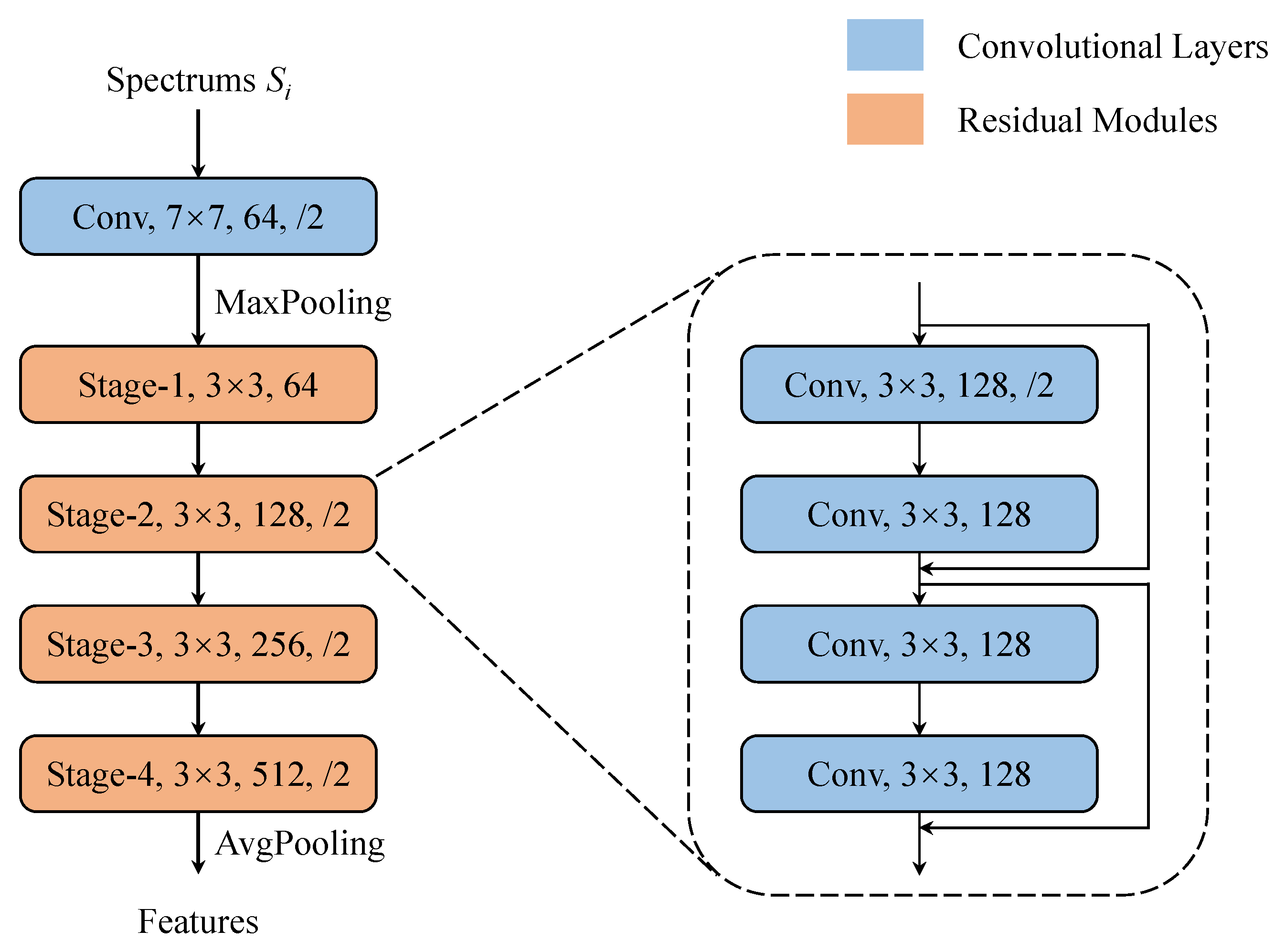
The baselines and our method were implemented with the PyTorch framework [44] and accelerated by an NVIDIA GeForce RTX 3090 Ti graphics card. During the optimization, the Adam optimizer [33] was employed to update the weights of CNN. For the fair comparison, the baselines adopted the same architecture of CNN as our method in Section 3.2, and the initialization of CNN weights and hyperparameters in optimization followed the default settings of PyTorch version 1.12.1. Moreover, for the baselines, utterances were preprocessed in the same way in Section 3.1 to obtain spectrums $S_i$ for further identification. Other settings about the training in this work were presented in

Table 3. Details of the training pipeline during the implementation.

Batch Size	Data Loader	Learning Rate	Scheduler	Maximum Epochs	Epoch for Early Stop
$NK-1$	Not Shuffle	$0.001$	$\times 0.95$ every 20 epochs	200	50

.

When evaluating the performance of the methods, we picked one utterance for each vessel to be identified for the training and tested the methods by using the utterances in other soundscapes that were different from the training one due to the receiving time of the hydrophone or working conditions of vessels. To quantify the identification performance, we employed the precision p, recall r, F1-score $F1$ and accuracy $Acc$, which were commonly used in the ship classification tasks. They were defined as in Equations (11) and (12):

$$p=\frac{TP}{TP+FP},r=\frac{TP}{TP+FN},F1=\frac{2·p·r}{p+r},$$

(11)

$$Acc=\frac{TP+TN}{TP+FP+TN+FN},$$

(12)

where true positive (TP) represented the utterances that were predicted to be the ship IDs of 1, and their actual IDs were also 1; false positive (FP) represented those that were predicted to be the ship IDs of 1, but their actual IDs were 0; false negative (FN) represented those that were predicted to be the ship IDs of 0, but their actual IDs were 1; while true negative (TN) represented those that were predicted to be the ship IDs of 0, and their actual IDs were also 0. For the multi-class identification, we calculated the macro average of these metrics by treating all classes equally. Moreover, we reported the confusion matrices on different identification tasks for the proposed method, which presented the rich information about the behavior of our method.

4.3. Performance for Different Settings of Ship Identification

The proposed method and the baselines were compared under the N-way K-shot framework with $K=5$. For the dataset SID1, 5 different passenger boats were required to be identified, so N was 5. The performance of these methods was shown in

Table 4. Performance results of methods on the SID1.

Methods	Macro-p	Macro-r	Macro-F1	Acc
SCNet	$0.392$	$0.258$	$0.224$	$0.258$
SiamNet	$0.511$	$0.485$	$0.467$	$0.485$
Proposed	$0.695$	$0.683$	$0.677$	$0.683$

. It could be seen that the performance of the conventional SCNet, which was usually used in the ship classification tasks, was limited because the available training samples were not enough. It was only slightly more accurate than the random guessing (with the accuracy of $0.26$ versus $0.20$). The performance of SiamNet adopting the contrastive learning strategy has been greatly improved (with the accuracy of $0.49$), but it was still not as good as our proposed method (with the accuracy of $0.68$). 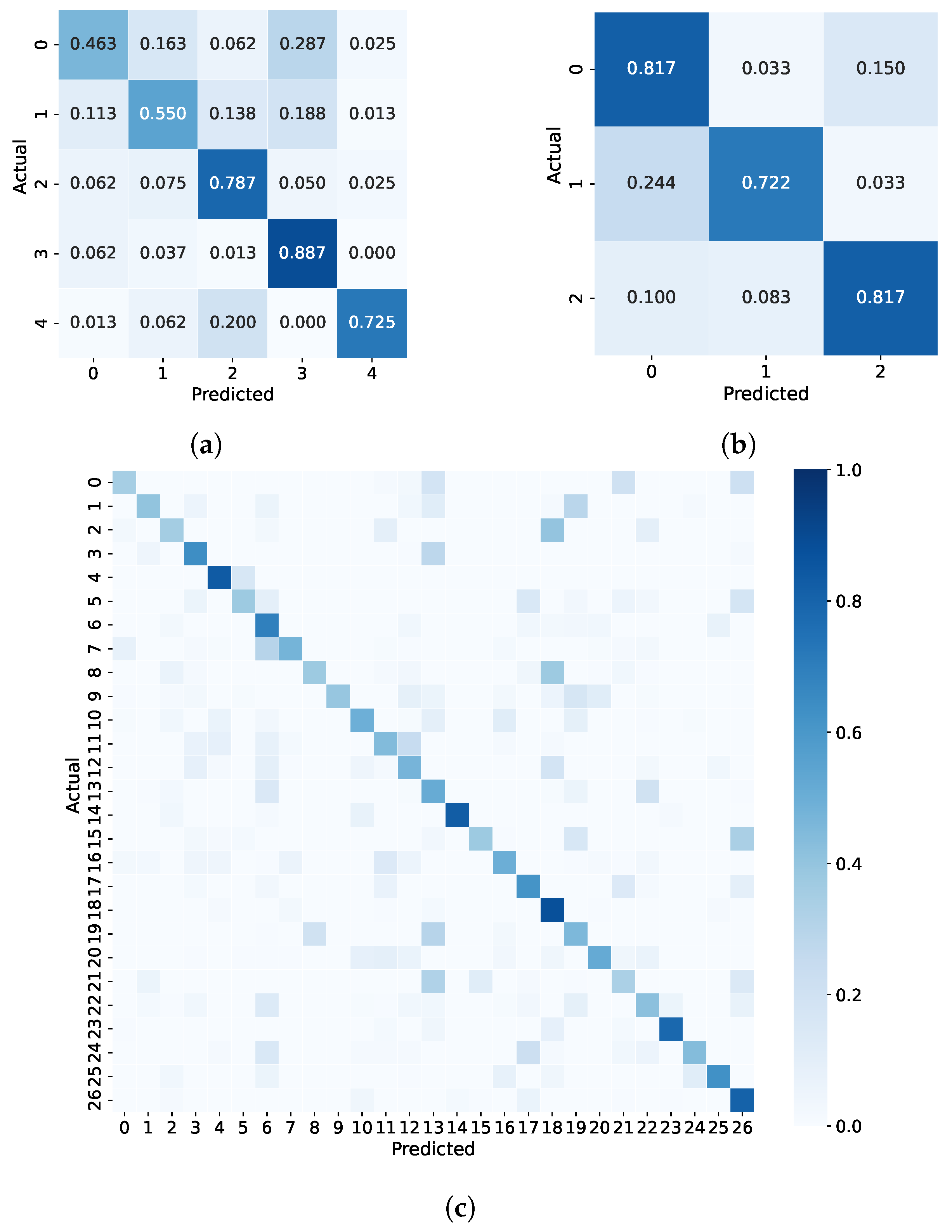The confusion matrix of the proposed method was also visualized in Figure 9a. The bright spots (with the high proportion) in the confusion matrix were almost along the diagonal of matrix, which showed that our method did work on the identification dataset, even though only 5 samples (10 s in total) were available.

Furthermore, in order to make the arguments more solid, we implemented the proposed method and the baselines on other identification datasets, SID2 and SID3, constructed from a completely independent sea trial data (VOS data) to discuss and compare their performance. The average results of precision, recall, F1-score and accuracy were listed in

Table 5. Performance results of methods on the SID2.

Methods	Macro-p	Macro-r	Macro-F1	Acc
SCNet	$0.445$	$0.343$	$0.186$	$0.343$
SiamNet	$0.710$	$0.680$	$0.677$	$0.680$
Proposed	$0.794$	$0.785$	$0.786$	$0.785$

and

Table 6. Performance results of methods on the SID3.

Methods	Macro-p	Macro-r	Macro-F1	Acc
SCNet	$0.140$	$0.151$	$0.131$	$0.151$
SiamNet	$0.408$	$0.330$	$0.328$	$0.330$
Proposed	$0.600$	$0.534$	$0.539$	$0.534$

, and the results on confusion matrices were shown in Figure 9b,c. The performance metrics of all methods were improved when the task difficulty dropped from 5-vessel identification to 3-vessel identification. However, SCNet still didn’t work due to limited training samples, its accuracy was almost the same as random guessing ($0.34$ versus $0.33$). The proposed method had the best performance on the SID2 regardless of which evaluation metric was focused. When the number of vessels to be identified increased from 5 to 27, the performance of all methods obviously decreased. This was reasonable since the ID pool of vessels was significantly enlarged and the methods needed to face more choices when classifying. On the SID3, accuracies of both SCNet and SiamNet dropped below $0.35$, while the proposed method achieved the accuracy over $0.5$ even on this challenging dataset. The diagonal distribution of bright spots in the confusion matrix also confirmed that the proposed method was still trustworthy under the 27-vessel identification task.

4.4. Target-Wise Performance of the Proposed Method

Next, the performance on each individual vessel of the proposed method in the ship identification task was discussed via the metrics of precision, recall and F1-score. And the high-dimensional features of each individual learned by our method were reduced in dimensionality by the t-SNE method [45] and then visualized. The discussions were based on numerical experiments carried out on the dataset, SID1, composed of the open-source real-world data.

The vessel-wise results of the proposed method on the SID1 were shown in

Table 7. Precision, recall and F1-score of each vessel of the proposed method on the SID1.

Vessels	Precision	Recall	F1-Score
i	$0.649$	$0.463$	$0.540$
ii	$0.620$	$0.550$	$0.583$
iii	$0.656$	$0.788$	$0.716$
iv	$0.628$	$0.888$	$0.736$
v	$0.921$	$0.725$	$0.811$

. It could be found that the identification performance of our method was varying for each vessel. The method identified vessels iii, iv and v very well, and the F1-scores for them were all above $0.7$. Comparatively, there were the poor performance for the proposed method when vessels i and ii were focused Even if the average metrics on the identification was close to $0.7$, the F1-scores for these two vessels were still below $0.6$.

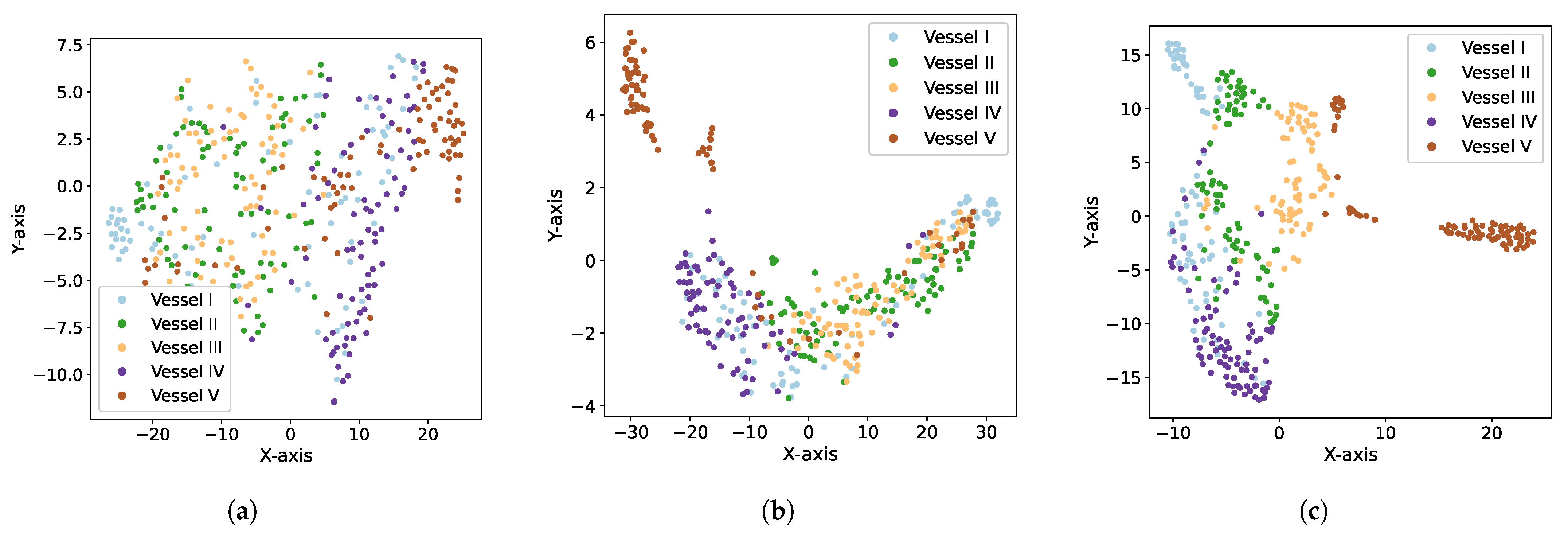
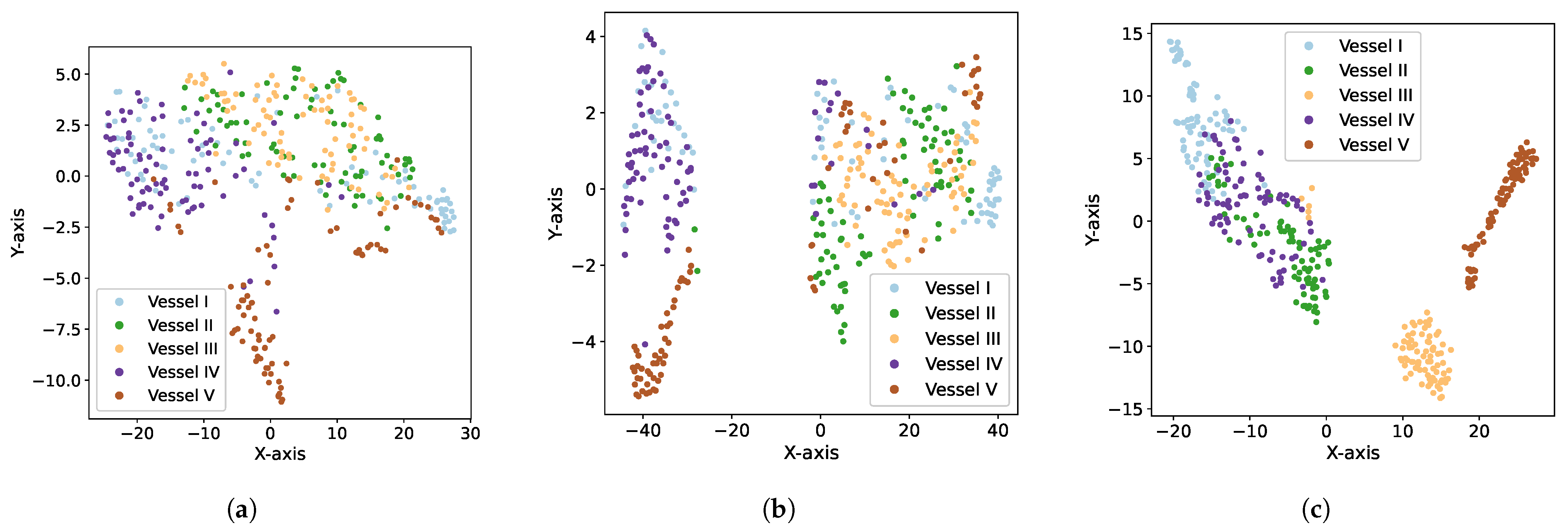
The visualization of the high-dimensional features in Figure 10 might be helpful to analyze the reasons behind the performance inconsistency on different vessels. With our training strategies, the feature extractor extracted the more discriminative features of vessels iii, iv and v, while for vessels i and ii, the obtained features were aliased with those of other vessel individuals (Figure 10a). Discrimination or not at the feature level led to differences in the behavior when identifying each vessel. Moreover, comparing with the features obtained from the conventional SCNet (Figure 10b) and the Siamese network SiamNet (Figure 10c), the proposed method was superiority in the training strategy of the feature extractor $\mathcal{F}$ with the same architecture, which prompted the model to put the features of the same vessel in different soundscapes together and keep those of the different vessels apart. SiamNet was also with the same intention, but it did not do this well from the visualized results, while the strategy of training the feature extractor with FC layers and the cross-entropy loss obviously failed in the few-shot scenario.

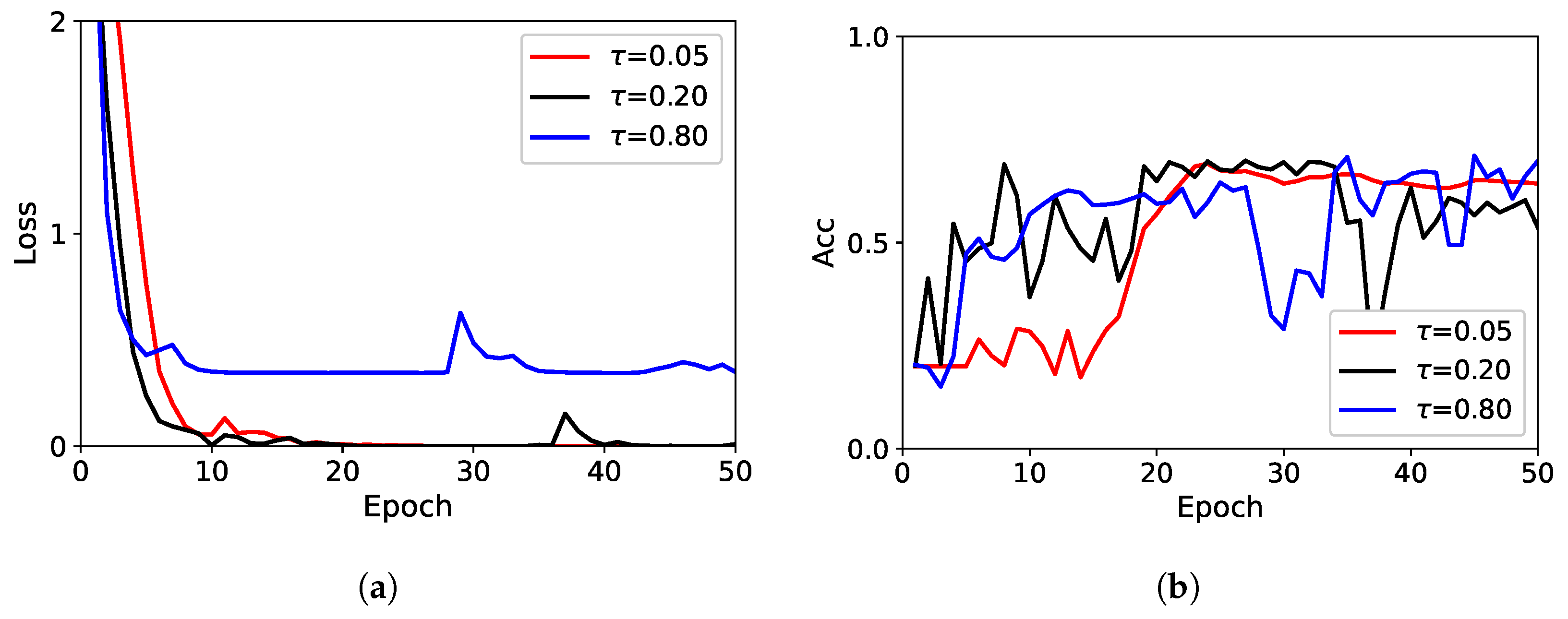
4.5. Convergence under Varying Hyperparameter $\tau$

As analyzed theoretically in Section 3.3, different values of the hyperparameter $\tau$ in Equation (6) affected the convergence of the proposed method during the training. The difference in convergence led to varying in the generalization performance of the model on the testing set. We empirically studied the difference in the convergence of the method caused by $\tau$ on the SID1 dataset. $\tau$ was set to $0.05$, $0.8$, and $0.2$, which represented undersized $\tau$, oversized $\tau$, and our default value, respectively. The loss of the method on the training set and the accuracy on the testing set were presented in Figure 11 with the increasing number of epochs in the training.

The convergence of the method was accelerated when $\tau$ increased, but the optimization for parameters in CNN also became unstable; meanwhile, too large $\tau$ also made the method converge on a high platform. For the generalization on the testing set, the different values of $\tau$ had little effect on the final performance of accuracy, and the best results that were achieved by the three $\tau$ showed almost no difference. However, a too small $\tau$ increased the number of epochs required for the method to achieve the good generalization, while a too large $\tau$ made it difficult to select a suitable number of epochs due to the unstable training. They could have an impact on how the proposed method behaved in practice.

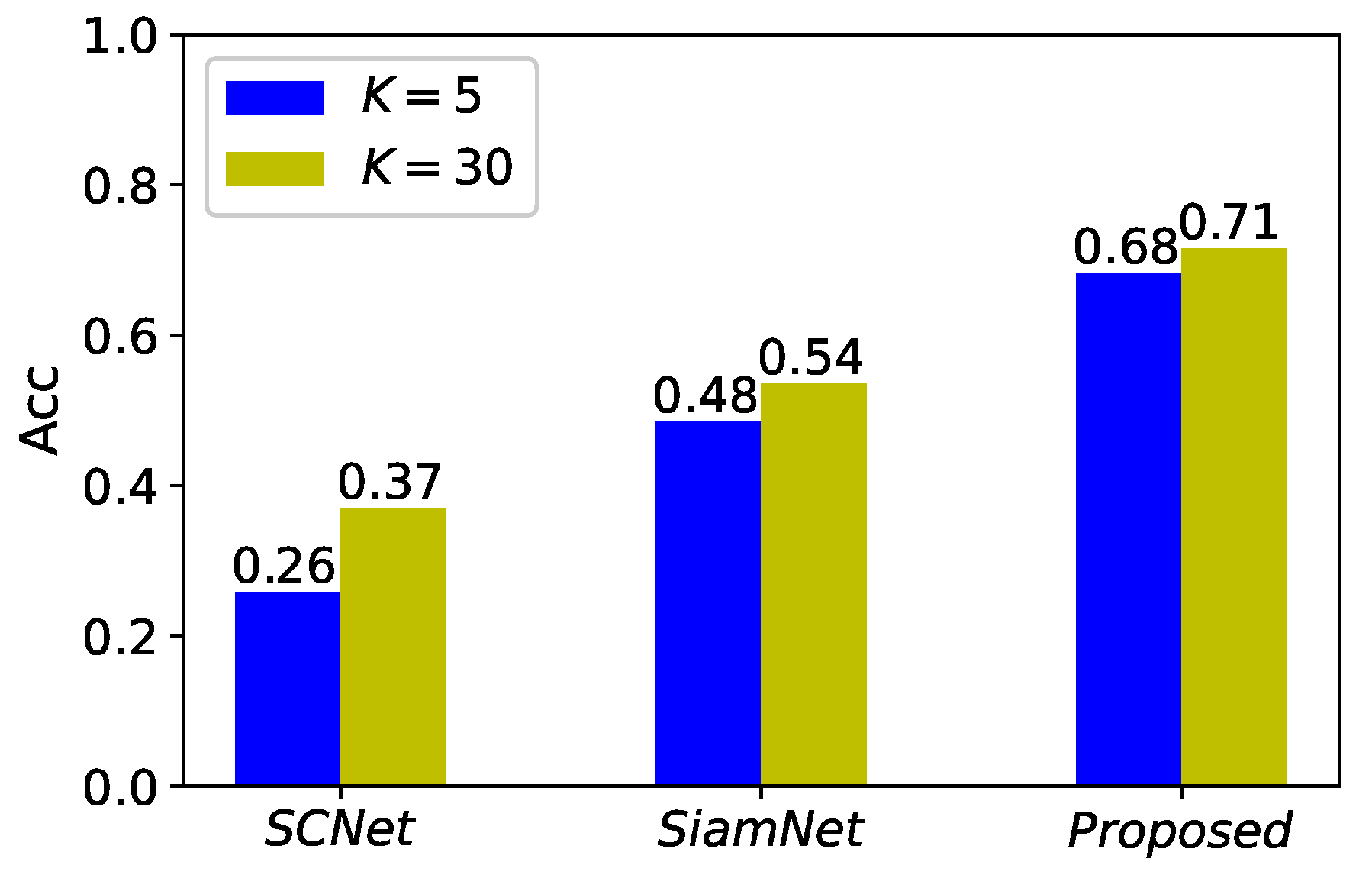
4.6. Performance versus the Number of Training Samples

Finally, we empirically discussed the changes brought by different values of K under the N-way K-shot setting to the ship identification task on the SID1. The performance on accuracy of the proposed method and baselines with $K=5$ and $K=30$ was shown in Figure 12. It could be found that more samples available for the training (caused by the increasing of K) improved the performance of all three methods, with the improvement on performance of SCNet being more significant than that of the contrastive learning methods.

The underlying reason might be that the classifier in SCNet consisting of FC layers was more sensitive to the increase in the number of data samples, while there were not the parameterized classifiers in the SiamNet and the proposed method, and therefore the performance gains from the increase in the available data were not as great for the latter two. The diversity brought by more real-world data allowed the methods to face more construction cases of sample-pairs during the training, and resulted in the improvement of feature extraction, which also promoted the final identification performance. Visualization of features learned by different methods when $K=30$ was also provided in Figure 13. Compared to Figure 10, the features learned by all methods were more discriminative than their own counterparts previously when the data available for the training was increased. Therefore, it could be argued that the performance gain brought to SCNet by the increase in training samples came from the coupling of both more distinguishable features and the more powerful classifier, while that brought to SiamNet and the proposed method was mainly from the first one. As a result, the performance gains of the latter two were smaller than that of the former.

4.7. Limitations and Future Works

In practice, port access verification or maritime security usually need to accurately identify whether the ship ID is a registered ID to provide a basis for the further response, where the limited data issue for each registered vessel should be considered as a major challenge. These tasks fit well with the few-shot ship identification discussed in this work, and the proposed method deals with it via adjusting the optimization objective of the training pipeline. There are some limitations for the practical application of the proposed method:

• Busy seas make multi-vessel interference almost inevitable, and the problem is simplified in this work by manually picking the interference-free moments of the vessels.
• The dataset constructed in this work employs the noises from near-field vessels, and how the acoustical distortion of noises from far-field vessels affect the identification performance needs further study.
• The evaluation in this work ensures generalization of the proposed method to both time- and space-variation in the same ocean because the constructed datasets in Section 4.1 are with temporal-separated utterances. However, it needs further investigation whether the method is still generalizable and what features can be re-used under the large-scale environmental changes caused by different target ocean.

5. Conclusions

In this work, we focused on the few-shot ship identification scenario, which aimed to utilize only a very few data samples (usually, smaller than 10 for each class) to develop a system that can automatically and accurately identify each vessel individuals that might be in different soundscapes. We made it well-defined with the N-way K-shot setting and proposed a contrastive-learning-based method for it. When training the model, it transformed the loss minimization between the prediction of samples with their labels into the maximization of similarity between positive pairs and minimization of that between negative pairs by constructing sample-pairs; and translated this multi-objective optimization into a solvable single-objective optimization via the InfoNCE loss. In the practical inference, a distance-based classifier was employed instead of the FC layers with numerous parameters; it avoided the training of the classifier that was difficult in few-shot applications by comparing the distance between the testing samples and the available registration templates on the feature space and assigning a testing sample as the ship ID of the registration templates closest to it.

The advantages of our method were validated on different sea-trial data. On the real-world tasks of 5-ship identification, 3-ship identification and 27-ship identification, the proposed method achieved the best performance with accuracies of $0.68$, $0.79$ and $0.53$; whereas the SCNet with conventional classification strategies only achieved accuracies of $0.26$, $0.34$ and $0.15$, and the SiamNet with classical contrastive strategies achieved accuracies of $0.49$, $0.68$ and $0.33$. The method was discussed in more detail on the 5-ship identification task. It was considered that the performance of our method on the identification of each individual vessel was inconsistent by the feature visualization and the vessel-wise analysis of identification results of the method. Furthermore, we also empirically studied the effect on convergence of the hyperparameter $\tau$ in our method and the potential gains for the methods from the increase of data samples available for the training. In conclusion, it could be argued that the proposed contrastive-learning-based ship identification method worked well in the real-world few-shot applications.

References

1. Arveson, P.T.; Vendittis, D.J. Radiated noise characteristics of a modern cargo ship. J. Acoust. Soc. Am. 2000, 107, 118–129. [Google Scholar] [CrossRef]
2. Pezeshki, A.; Azimi-Sadjadi, M.R.; Scharf, L.L. Undersea target classification using canonical correlation analysis. IEEE J. Ocean. Eng. 2007, 32, 948–955. [Google Scholar] [CrossRef] [Green Version]
3. Bianco, M.J.; Gerstoft, P.; Traer, J.; Ozanich, E.; Roch, M.A.; Gannot, S.; Deledalle, C.A. Machine learning in acoustics: Theory and applications. J. Acoust. Soc. Am. 2019, 146, 3590–3628. [Google Scholar] [CrossRef] [PubMed] [Green Version]
4. Bao, F.; Li, C.; Wang, X.; Wang, Q.; Du, S. Ship classification using nonlinear features of radiated sound: An approach based on empirical mode decomposition. J. Acoust. Soc. Am. 2010, 128, 206–214. [Google Scholar] [CrossRef]
5. Wang, S.; Zeng, X. Robust underwater noise targets classification using auditory inspired time–frequency analysis. Appl. Acoust. 2014, 78, 68–76. [Google Scholar]
6. Ke, X.; Yuan, F.; Cheng, E. Integrated optimization of underwater acoustic ship-radiated noise recognition based on two-dimensional feature fusion. Appl. Acoust. 2020, 159, 107057. [Google Scholar] [CrossRef]
7. Nie, L.; Li, C.; Wang, H.; Marzani, F. Open-Set Recognition for Deep Neural Networks-based Underwater Acoustic Target Classification. In Proceedings of the OCEANS 2021, San Diego, CA, USA, 20–23 September 2021; pp. 1–5. [Google Scholar]
8. Luo, X.; Zhang, M.; Liu, T.; Huang, M.; Xu, X. An Underwater Acoustic Target Recognition Method Based on Spectrograms with Different Resolutions. J. Mar. Sci. Eng. 2021, 9, 1246. [Google Scholar] [CrossRef]
9. Ren, J.; Xie, Y.; Zhang, X.; Xu, J. UALF: A learnable front-end for intelligent underwater acoustic classification system. Ocean. Eng. 2022, 264, 112394. [Google Scholar] [CrossRef]
10. Neupane, D.; Seok, J. A review on deep learning-based approaches for automatic sonar target recognition. Electronics 2020, 9, 1972. [Google Scholar] [CrossRef]
11. Das, A.; Kumar, A.; Bahl, R. Marine vessel classification based on passive sonar data: The cepstrum-based approach. IET Radar Sonar Navig. 2013, 7, 87–93. [Google Scholar] [CrossRef]
12. Beckler, B.; Pfau, A.; Orescanin, M.; Atchley, S.; Villemez, N.; Joseph, J.E.; Miller, C.W.; Margolina, T. Multilabel Classification of Heterogeneous Underwater Soundscapes With Bayesian Deep Learning. IEEE J. Ocean. Eng. 2022, 47, 1143–1154. [Google Scholar] [CrossRef]
13. Howe, B.M.; Miksis-Olds, J.; Rehm, E.; Sagen, H.; Worcester, P.F.; Haralabus, G. Observing the oceans acoustically. Front. Mar. Sci. 2019, 6, 426. [Google Scholar] [CrossRef] [Green Version]
14. Doan, V.S.; Huynh-The, T.; Kim, D.S. Underwater acoustic target classification based on dense convolutional neural network. IEEE Geosci. Remote. Sens. Lett. 2020, 19, 1–5. [Google Scholar] [CrossRef]
15. Chen, Y.; Liang, H.; Pang, S. Study on small samples active sonar target recognition based on deep learning. J. Mar. Sci. Eng. 2022, 10, 1144. [Google Scholar] [CrossRef]
16. Xiao, X.; Wang, W.; Ren, Q.; Gerstoft, P.; Ma, L. Underwater acoustic target recognition using attention-based deep neural network. JASA Express Lett. 2021, 1, 106001. [Google Scholar] [CrossRef] [PubMed]
17. Khishe, M. DRW-AE: A Deep Recurrent-Wavelet Autoencoder for Underwater Target Recognition. IEEE J. Ocean. Eng. 2022, 47, 1083–1098. [Google Scholar] [CrossRef]
18. Li, P.; Wu, J.; Wang, Y.; Lan, Q.; Xiao, W. STM: Spectrogram Transformer Model for Underwater Acoustic Target Recognition. J. Mar. Sci. Eng. 2022, 10, 1428. [Google Scholar] [CrossRef]
19. Yang, H.; Xu, G.; Yi, S.; Li, Y. A new cooperative deep learning method for underwater acoustic target recognition. In Proceedings of the OCEANS 2019, Marseille, France, 17–20 June 2019; pp. 1–4. [Google Scholar]
20. Liu, F.; Shen, T.; Luo, Z.; Zhao, D.; Guo, S. Underwater target recognition using convolutional recurrent neural networks with 3-D Mel-spectrogram and data augmentation. Appl. Acoust. 2021, 178, 107989. [Google Scholar] [CrossRef]
21. He, L.; Shen, X.; Zhang, M.; Wang, H. Discriminative Ensemble Loss for Deep Neural Network on Classification of Ship-Radiated Noise. IEEE Signal Process. Lett. 2021, 28, 449–453. [Google Scholar] [CrossRef]
22. McKenna, M.F.; Ross, D.; Wiggins, S.M.; Hildebrand, J.A. Underwater radiated noise from modern commercial ships. J. Acoust. Soc. Am. 2012, 131, 92–103. [Google Scholar] [CrossRef] [Green Version]
23. Yang, H.; Li, J.; Shen, S.; Xu, G. A deep convolutional neural network inspired by auditory perception for underwater acoustic target recognition. Sensors 2019, 19, 1104. [Google Scholar] [CrossRef] [PubMed] [Green Version]
24. Parsons, M.J.; Erbe, C.; Meekan, M.G.; Parsons, S.K. A review and meta-analysis of underwater noise radiated by small (<25 m length) vessels. J. Mar. Sci. Eng. 2021, 9, 827. [Google Scholar]
25. Vinyals, O.; Blundell, C.; Lillicrap, T.; Kavukcuoglu, K.; Wierstra, D. Matching Networks for One Shot Learning. In Proceedings of the Advances in Neural Information Processing Systems, Barcelona, Spain, 5–10 December 2016; Volume 29, pp. 1–9. [Google Scholar]
26. Snell, J.; Swersky, K.; Zemel, R. Prototypical networks for few-shot learning. In Proceedings of the Advances in Neural Information Processing Systems, Long Beach, CA, USA, 4–9 December 2017; Volume 30, pp. 1–11. [Google Scholar]
27. Miao, Y.; Zakharov, Y.V.; Sun, H.; Li, J.; Wang, J. Underwater acoustic signal classification based on sparse time–frequency representation and deep learning. IEEE J. Ocean. Eng. 2021, 46, 952–962. [Google Scholar] [CrossRef]
28. Krizhevsky, A.; Sutskever, I.; Hinton, G.E. ImageNet Classification with Deep Convolutional Neural Networks. In Proceedings of the Advances in Neural Information Processing Systems, Lake Tahoe, NV, USA, 3–8 December 2012; Volume 25, pp. 1097–1105. [Google Scholar]
29. Goodfellow, I.; Bengio, Y.; Courville, A. Deep Learning; MIT Press: Cambridge, MA, USA, 2016. [Google Scholar]
30. Guo, C.; Pleiss, G.; Sun, Y.; Weinberger, K.Q. On calibration of modern neural networks. In Proceedings of the International Conference on Machine Learning, Sydney, NSW, Australia, 6–11 August 2017; pp. 1321–1330. [Google Scholar]
31. Rasmussen, C.E.; Williams, C.K. Gaussian Processes for Machine Learning; Springer: Berlin/Heidelberg, Germany, 2006; Volume 1. [Google Scholar]
32. Rumelhart, D.E.; Hinton, G.E.; Williams, R.J. Learning representations by back-propagating errors. Nature 1986, 323, 533–536. [Google Scholar] [CrossRef]
33. Kingma, D.P.; Ba, J. Adam: A Method for Stochastic Optimization. In Proceedings of the 3rd International Conference on Learning Representations, San Diego, CA, USA, 7–9 May 2015. [Google Scholar]
34. Zhou, Z.H. Why over-parameterization of deep neural networks does not overfit? Sci. China Inf. Sci. 2021, 64, 1–3. [Google Scholar] [CrossRef]
35. He, K.; Zhang, X.; Ren, S.; Sun, J. Deep residual learning for image recognition. In Proceedings of the IEEE Conference on Computer Vision and Pattern Recognition, Las Vegas, NV, USA, 27–30 June 2016; pp. 770–778. [Google Scholar]
36. Chen, T.; Kornblith, S.; Norouzi, M.; Hinton, G. A simple framework for contrastive learning of visual representations. In Proceedings of the International Conference on Machine Learning, Online, 13–18 July 2020; pp. 1597–1607. [Google Scholar]
37. Oord, A.V.D.; Li, Y.; Vinyals, O. Representation learning with contrastive predictive coding. arXiv 2018, arXiv:1807.03748. [Google Scholar]
38. Wang, F.; Liu, H. Understanding the behaviour of contrastive loss. In Proceedings of the IEEE/CVF Conference on Computer Vision and Pattern Recognition, Nashville, TN, USA, 20–25 June 2021; pp. 2495–2504. [Google Scholar]
39. Wang, T.; Isola, P. Understanding contrastive representation learning through alignment and uniformity on the hypersphere. In Proceedings of the International Conference on Machine Learning, Online, 13–18 July 2020; pp. 9929–9939. [Google Scholar]
40. Chen, X.; He, K. Exploring simple siamese representation learning. In Proceedings of the IEEE/CVF Conference on Computer Vision and Pattern Recognition, Nashville, TN, USA, 20–25 June 2021; pp. 15750–15758. [Google Scholar]
41. Santos-Domínguez, D.; Torres-Guijarro, S.; Cardenal-López, A.; Pena-Gimenez, A. ShipsEar: An underwater vessel noise database. Appl. Acoust. 2016, 113, 64–69. [Google Scholar] [CrossRef]
42. Irfan, M.; Jiangbin, Z.; Ali, S.; Iqbal, M.; Masood, Z.; Hamid, U. DeepShip: An underwater acoustic benchmark dataset and a separable convolution based autoencoder for classification. Expert Syst. Appl. 2021, 183, 115270. [Google Scholar] [CrossRef]
43. Liu, D.; Shen, W.; Cao, W.; Hou, W.; Wang, B. Design of Siamese Network for Underwater Target Recognition with Small Sample Size. Appl. Sci. 2022, 12, 10659. [Google Scholar] [CrossRef]
44. Paszke, A.; Gross, S.; Massa, F.; Lerer, A.; Bradbury, J.; Chanan, G.; Killeen, T.; Lin, Z.; Gimelshein, N.; Antiga, L.; et al. Pytorch: An imperative style, high-performance deep learning library. In Proceedings of the Advances in Neural Information Processing Systems, Vancouver, BC, Canada, 8–14 December 2019; Volume 32, pp. 8024–8035. [Google Scholar]
45. Van der Maaten, L.; Hinton, G. Visualizing Data using t-SNE. J. Mach. Learn. Res. 2008, 9, 2579–2605. [Google Scholar]
Figure 1. Divisions for categories of source vessels in tasks of ship classification and ship identification from the received noises: (a) Dividing noises to several categories (I–IV in the figure) based on the purpose of source vessels in the ship classification. (b) Dividing noises to each source individual (I–XII in the figure) in the ship identification.
Jmse 11 00782 g001
Figure 2. Pipeline of machine-learning-based methods for solving tasks of ship classification or identification from the received ship-radiated noises.
Jmse 11 00782 g002
Figure 3. Diagram of the proposed contrastive-learning-based methods for the task of few-shot ship identification. The CNN was parameter-shared, while the classifier was parameter-free.
Jmse 11 00782 g003
Figure 4. Architecture of ResNet-18 employed in the proposed methods, where each stage consisted of 4 convolutional layers (with the same kernel size and channel number) and 2 residual connections. “Conv, 7 × 7 , 64, / 2 ” meant that a 2D convolutional operator with the kernel size of 7 × 7 , the output channel number of 64, and the stride of 2 (the default stride was 1) was employed in the layer.
Jmse 11 00782 g004
Figure 5. Illustration of increasing and decreasing of similarity in the feature space for our contrastive-learning-based methods.
Jmse 11 00782 g005
Figure 6. Mechanism of the distance-based classifier. It provided the classification results of testing samples by utilized the registration templates in the feature space without the parameterized FC layers or logistic regression.
Jmse 11 00782 g006
Figure 7. Details of the sea trials in the northern South China Sea: (a) Schematic sketch of the sea trials. (b) A sound speed profile case in the experimental sea area.
Jmse 11 00782 g007
Figure 8. Graphical representation on the composition of VOS data and some examples of the time-frequency spectrums of utterances.
Jmse 11 00782 g008
Figure 9. The results on the confusion matrices for the proposed method: (a) on the SID1. (b) on the SID2. (c) on the SID3.
Jmse 11 00782 g009
Figure 10. Visualization for the high-dimensional features in different methods via the t-SNE: (a) SCNet. (b) SiamNet. (c) Proposed.
Jmse 11 00782 g010
Figure 11. Convergence and generalization of the proposed method with varying τ : (a) Loss on the training set of SID1. (b) Accuracy on the testing set of SID1.
Jmse 11 00782 g011
Figure 12. Accuracies of methods with different numbers of data samples available for the training ( K = 5 and K = 30 under the N-way K-shot setting).
Jmse 11 00782 g012
Figure 13. Visualization for the features learned by different methods when the number K of training samples was 30: (a) SCNet. (b) SiamNet. (c) Proposed.
Jmse 11 00782 g013