Study of Phytoplankton Biomass and Environmental Drivers in and around the Ross Sea Marine Protected Area

Abstract

The Southern Ocean plays a vital role in the global climate system and the life cycle of high-latitude marine life. Phytoplankton is an important source of primary productivity in this ecosystem. Its future changes could affect Southern Ocean geochemistry, carbon export, and higher trophic organisms. To better protect Antarctica, three different marine protected areas (MPA) have been established in the Ross Sea region. Because time-continuous and regionally complete data are difficult to obtain in this region, we obtained data from ocean model outputs to understand the spatiotemporal variability of phytoplankton biomass in this region. This study explored the correlation between phytoplankton biomass and key environmental factors. Phytoplankton biomass peaks in February as temperatures rise and sea ice melts. Correlations also vary between different protected areas. The correlation between biomass, nitrate, and salinity in the Krill Research Zone (KRZ) area was significantly different from other protected areas. In addition, in the context of global warming, Antarctica lacks temperature perception. The model results show a downward trend in temperature and an increase in sea ice coverage in the western Ross Sea that other studies have also pointed to. How phytoplankton biomass will change in protected areas in the future is a question worth considering. Finally, the study simply simulates future regional trends by comparing the biomass distribution in hot years to average years. This will increase our knowledge of the polar system.

1. Introduction

The Ross Sea (77° S and 175° W) extends from Cape Adare in the west to Cape Colbeck in the east [1]. It has two key components: the continental shelf (the most extensive in the Antarctic) and the continental slope. The region is widely considered to be one of the last ecosystems on Earth that are virtually undisturbed by humans [2]. However, the climate anomalies have led to recent changes in the formation of Antarctic bottom water [3] and a rebound in the salinity of shelf water [4]. Therefore, as a “natural laboratory”, the Ross Sea is an ideal place to study climate change and its effects. Since 2018, it has established marine protected areas (MPA) in international waters (150,000 km²) [5]. The Ross Sea is also one of the most unique and complex marine ecosystems in Antarctica. Special characteristics of the Ross Sea include a series of natural and physical characteristics in the neritic (coastal) and benthic (seafloor) zones, there is a diverse biota, including extremely high levels of endemism [6,7]. It has a strong influence on marine biogeochemical cycles as well as air-sea heat and CO₂ fluxes on a global scale [8].

Over the past 37 years, since the advent of regular satellite passive microwave observation of sea ice, there has been a small but statistically significant increase in overall Southern Ocean sea ice coverage [9,10]. This trend is dominated by increased sea ice coverage in the western Ross Sea. The atmosphere is considered to be the main driving force of these observed trends, but the ocean is also important in explaining the seasonality of trend patterns. Detecting an anthropogenic signal in Antarctic sea ice is particularly challenging because the expected response is small compared to the very high natural variation of the system and the observation record is relatively short. Due to the complex climate system of Antarctica, the ability of the global coupled climate model is also questioned [11]. The climate is variously predicted to experience increased warming, stronger winds, acidification, shallower mixing depths, increased light (and ultraviolet light), changes in upwelling and nutrient replenishment, reduced sea ice, reduced salinity, and the southward shift of ocean frontiers. These changes are expected to alter the structure and function of Marine phytoplankton communities [12]. The microbial community in the Southern Ocean broadly comprises phytoplankton, bacteria, flagellates, and ciliates. Phytoplankton in the coastal waters of Antarctica grows faster than in the more distant offshore waters [13]. The effect of light [14] and the supply of dissolved iron and other trace elements [15] can affect the growth of phytoplankton. Some phytoplankton, such as prymnesiophytes and dinoflagellates can affect the cloud cover and atmospheric albedo over the Southern Ocean, thereby changing the global heat balance [12]. This is caused by the release of plankton metabolites, such as dimethyl sulfide [16]. This shows that there may be interactions between phytoplankton and the environment. Generally, the first bloom of phytoplankton occurs in early spring. There will often be a secondary peak in summer [17]. Because phytoplankton multiplies rapidly under optimal growth conditions (i.e., high nutrient levels, ideal light, temperature, and minimal losses from grazing and vertical mixing) [18] the combined action of melting ice and wind will increase the stratification of the ocean surface, which may lead to the proliferation of phytoplankton [19]. When sea ice melts, it may release nutrients, especially the micronutrient iron, and it may promote blooms of ice algae in the water column [20]. Understanding the response of marine phytoplankton to climate change is essential for predicting the future state of marine ecosystems, estimating the impact of marine ecosystems on fisheries and endangered species, and accurately predicting the impact of physical and biological changes in marine ecosystems on global climate. The predicted changes in the phytoplankton community may affect the Southern Ocean biogeochemistry, carbon export, and nutrition for higher trophic levels [12].

The MPA is the result of unanimous support for a joint New Zealand/US proposal within the 25-member Council for the Conservation of Marine Living Resources (CCAMLR) for environmental protection, sustainable fisheries, and scientific interests in the Ross Sea. In 2012, New Zealand and the United States made a joint proposal for marine protected areas for the first time, and the two parties reached an agreement in October 2016. On 1 December 2017, the agreement on this marine protected area came into effect. The Ross Sea MPA is the world’s largest marine protected area of the Antarctic and covers a stretch of water twice the size of the US state of Texas about 1.55 million square kilometers (https://www.mfat.govt.nz/ (accessed on 20 November 2022)). There are three different types of the Ross Sea MPA: “General Protection Zone”, split into three separate areas, is fully protected with no commercial fishing permitted; “Krill Research Zone”, which allows for controlled research into krill fishing with the aim of the MPA; and “Special Research Zone”, which allows for limiting research fishing for krill and toothfish.

Several previous studies have assessed temporal and spatial patterns of phytoplankton biomass, productivity, and particulate matter composition in the Ross Sea. Smith et al. (1996) found that the primary determinant of phytoplankton biomass and productivity at any point on the Ross Sea shelf is the phase of the seasonal growth cycle [21]. The Southern Ocean is a high nutrient, low chlorophyll (HNLC) system because the lack of micronutrients such as iron limits phytoplankton growth and is subject to complex plankton bloom processes [22,23]. The iron limitation is related to low primary productivity [24]. When the Antarctic circumpolar current (ACC) fronts separate water masses, every mass has different physical properties and lead plankton, nutrient, and iron concentrations [25] and have a big impact on the intensity of blooms. Reddy et al. (2006) concluded from model studies that phytoplankton distributions can be constrained by the interaction of deep bathymetry and surface geostrophic currents along the highly productive Antarctic continental shelf.

Antarctic coastal waters represent a special kind of ecosystem because of sea ice. Not only does it provide a stable habitat for phytoplankton, but it also affects Antarctic circulation. As primary producers, understanding the distribution, abundance, and drivers of phytoplankton communities is critical to the conservation of Antarctic ecology. Our research will be based on model data from the Australian Community Climate and Earth System Simulator (ACCESS) to examine spatial and temporal trends in phytoplankton biomass and environmental factors in the Ross Sea over 50 years and to analyze differences in correlations and spatial variability between environmental variables in different Ross Sea protected areas. The study explores trends in phytoplankton biomass in MPA in the context of future global warming. Our results can help better conserve, develop, and utilize Antarctic ecology and resources in the future. The manuscript is organized as follows: Section 1 introduces the basic situation of the Ross Sea in Antarctica, the importance of phytoplankton, and also the background of CCAMLR’s establishment of MPA in the Ross Sea. Section 2 introduces the environmental variable data from the sea ice model, biomass data from the biogeochemistry model, and the method. Section 3 describes the change trend and distribution of biomass and environmental variables, and the correlation between them is analyzed. Finally, by comparing the differences between warm years and average years, the changes in biomass and the Ross Sea environment after climate warming are predicted. Section 4 and Section 5 provide a discussion and conclusions.

2. Materials and Methods

2.1. Data Sources

This study focuses on the effects of environmental variables on phytoplankton biomass. Data included phytoplankton biomass, sea temperature, salinity, sea ice concentration, and nitrate concentration, all from the Consortium for Ocean-Sea Ice Modelling in Australia (COSIMA). The ACCESS-OM2 model has three different horizontal resolutions: a coarse resolution (nominally 1° horizontal grid spacing), an eddy-permitting resolution (nominally 0.25°), and an eddy-rich resolution (0.1° with 75 vertical levels). It is suitable for studies investing in the sensitivity of solutions to model resolution. Every level of resolution has advantages and disadvantages. In this research, we use 0.25° latitude resolution from 60.6° S to 77.9° S and 1° longitude resolution from 150.5° E to 150.5° W from 1958 to 2018 (https://dapds00.nci.org.au/thredds/catalogs/cj50/access-om2/access-om2.html (accessed on 8 March 2023)). The data size is 60 × 43 × 50 × 12 × 61 (longitude, latitude, layers, month, years). Since sea ice only has surface data, only the first layer (surface layer) of other variables is selected for correlation analysis in order to carry out the unified analysis. More descriptions of the model data can be found on the COSIMA website (https://cosima.org.au/ (accessed on 8 March 2023)). Further details on version 1.0 of the model are available in Kiss et al. (2020). The latest model code and standard configurations are available via https://github.com/COSIMA/access-om2 (accessed on 8 March 2023).

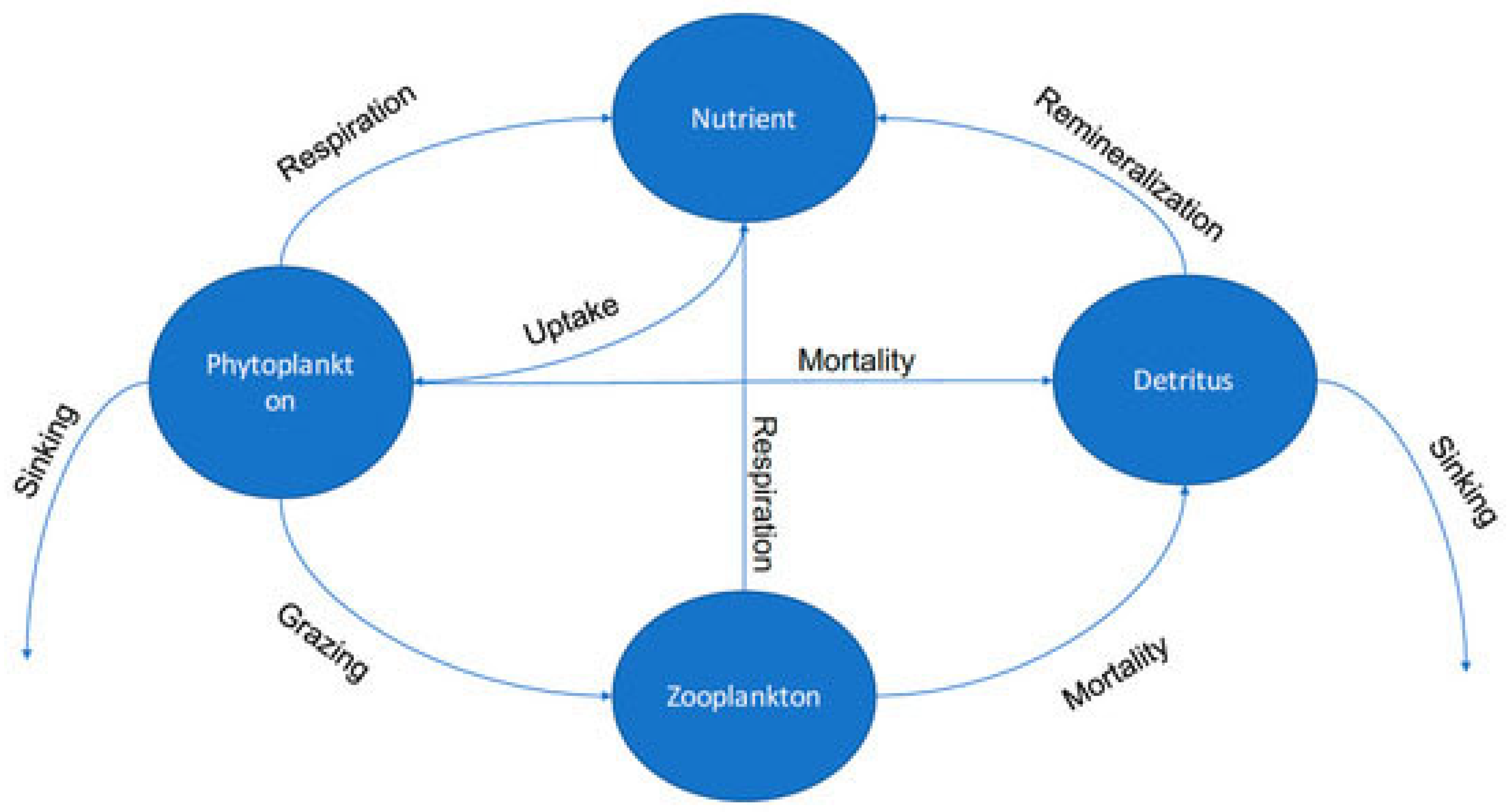
2.2. Model Description

The sea ice data in this study are derived from COSIMA’s 1/4° ocean sea ice model, the Australian Community Climate, and the Earth-System Simulator (ACCESS-OM2-025) [26]. It comprises the MOM5.1 ocean model coupled to the CICE5.1.2 sea ice model via OASIS3-MCT. The model is global, but this study focused only on the Antarctic Ross Sea. The ocean sea ice model coupled climate and Earth system can be used for predicting the future climate, and biogeochemical and ecosystem dynamics can also be incorporated [27]. Specifically, the whole ocean model with biogeochemistry and trophic-dynamics (WOMBAT) in the ACCESS-OM2 model [28]. Our environmental variables and phytoplankton biomass data are derived from this model, the Australian Marine Forecast Model Version 3 (OFAM3), developed by CSIRO, the Bureau of Meteorology (BoM) and the Royal Australian Navy. The biological model is called the whole ocean model with biogeochemistry and trophic-dynamics (WOMBAT), one of the biogeochemical cycles models in OFAM3 [29]. In brief, WOMBAT is a three-dimensional NPZD model (nutrient–phytoplankton–zooplankton–detritus) described by Kidston, Matear, and Baird (2011). The NPZD model can describe the functions of the ecosystem in detail by reproducing the movement of energy in the low trophic levels of the food web. It is a nitrogen-based model. Due to the need for fewer parameters and observation data, the NPZD ecological model is currently one of the most popular models [30]. Many ecological and physical processes in different sea areas have been successfully simulated. For more information on the model and configuration see Kiss et al. (2020), Oke et al. (2013), and Kidston, Matear, and Baird (2011) [26,28,29]. Below are the four basic modules of the model (Figure 1).

There are four equations in any NPZD (1)–(4) that describe dissolved inorganic nitrogen (N), phytoplankton biomass (P), herbivorous zooplankton biomass (Z), and detritus (D). Depending on the implementation, the specifics of these equations change, but they are always similar to the equation below [32]. (Parameter are defined in

Table 1. Parameters in the NPZD model.

Parameter	Symbol
Quadratic mortality rate (Phytoplankton coefficients)	${\mathsf{\mu }}_{\mathrm{p}}^2$
Remineralization rate (Detrital coefficients)	${\mathsf{\mu }}_{\mathrm{D}}$
Quadratic mortality rate (Zooplankton coefficients)	${\mathsf{\mu }}_{\mathrm{Z}}$
Sinking velocity (Detrital coefficients)	${\mathrm{w}}_{\mathrm{D}}$
Assimilation efficiency (Zooplankton coefficients)	${\mathsf{\gamma }}_1$
Excretion rate (Zooplankton coefficients)	${\mathsf{\gamma }}_2$
The nitrogen concentration below the mixed layer	${\mathrm{N}}_0$

).

$$\frac{\mathrm{dN}}{\mathrm{dt}}={\mathsf{\mu }}_{\mathrm{D}}\mathrm{D}+{\gamma }_2\mathrm{Z}- \overline{\mathrm{J}}\left(\mathrm{M},\mathrm{t},\mathrm{N}\right)\mathrm{P}+\frac{\mathrm{w}+\left(\mathrm{t}\right)\left({\mathrm{N}}_0-\mathrm{N}\right)}{\mathrm{M}}$$

(1)

$$\frac{\mathrm{dP}}{\mathrm{dt}}= \overline{\mathrm{J}}\left(\mathrm{M},\mathrm{t},\mathrm{N}\right)\mathrm{P}-\mathrm{G}\left(\mathrm{P}\right)\mathrm{Z}-{\mathsf{\mu }}_{\mathrm{p}}^2{\mathrm{P}}^2-\frac{\mathrm{w}+\left(\mathrm{t}\right)\mathrm{P}}{\mathrm{M}}$$

(2)

$$\frac{\mathrm{dZ}}{\mathrm{dt}}={\gamma }_1\mathrm{G}\left(\mathrm{P}\right)\mathrm{Z}-{\gamma }_2\mathrm{Z}-{\mathsf{\mu }}_{\mathrm{Z}}{\mathrm{Z}}^2-\frac{\mathrm{w}\left(\mathrm{t}\right)\mathrm{Z}}{\mathrm{M}}$$

(3)

$$\frac{\mathrm{dD}}{\mathrm{d}}=\left(1-{\gamma }_1\right)\mathrm{G}\left(\mathrm{P}\right)\mathrm{Z}+{\mathsf{\mu }}_{\mathrm{Z}}{\mathrm{Z}}^2+{\mathsf{\mu }}_{\mathrm{p}}^2{\mathrm{P}}^2-{\mathsf{\mu }}_{\mathrm{D}}\mathrm{D}-\frac{\left({\mathrm{w}}_{\mathrm{D}}+\mathrm{w}+\left(\mathrm{t}\right)\right)\mathrm{P}}{\mathrm{M}}$$

(4)

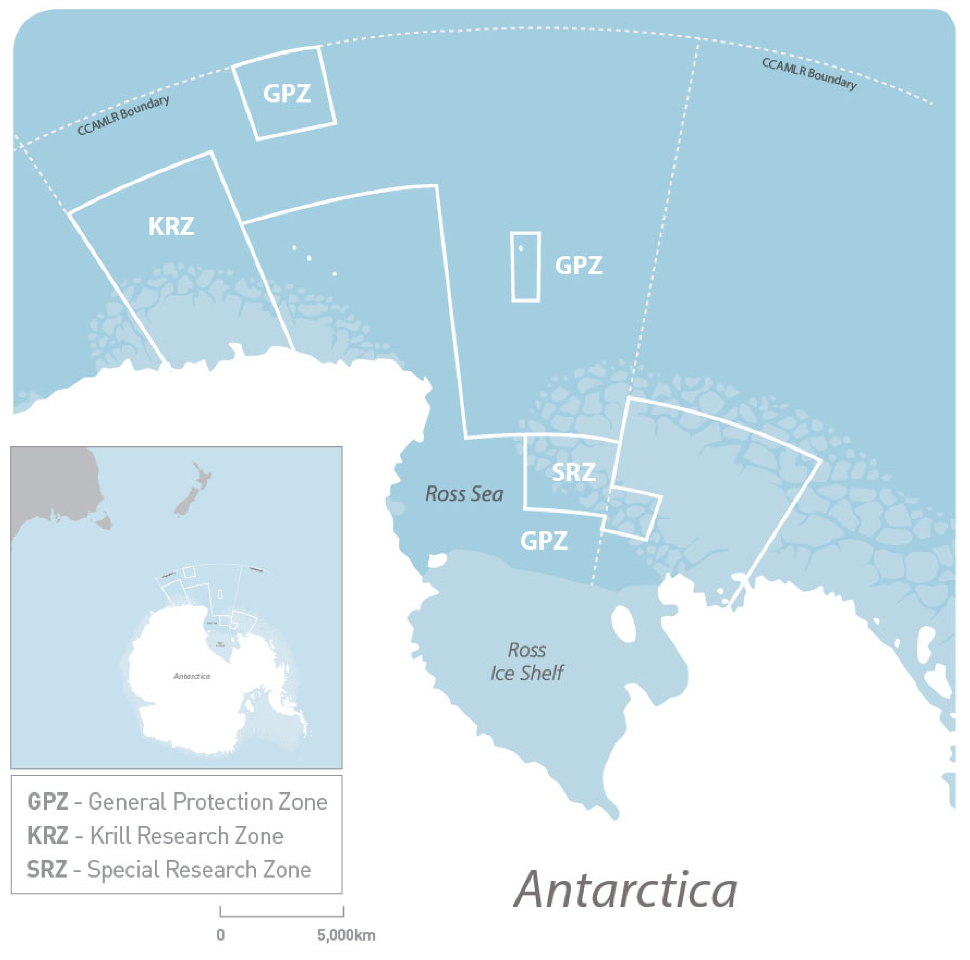
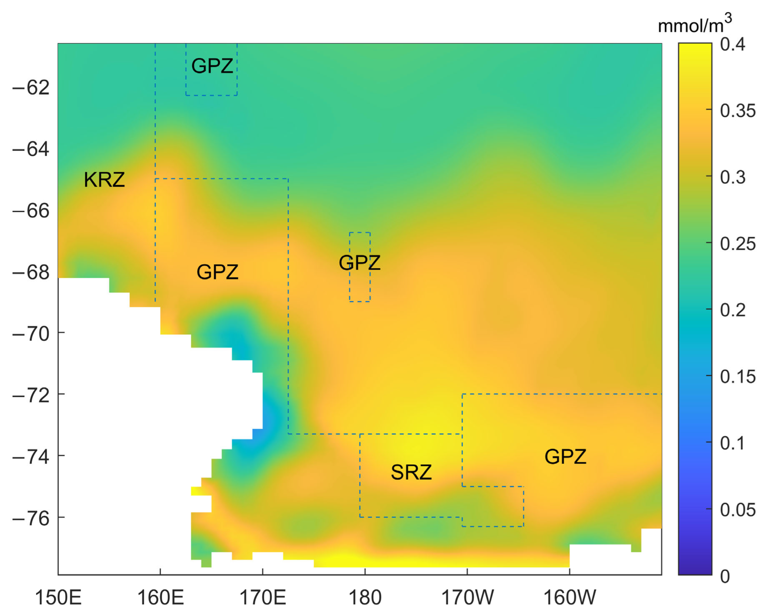
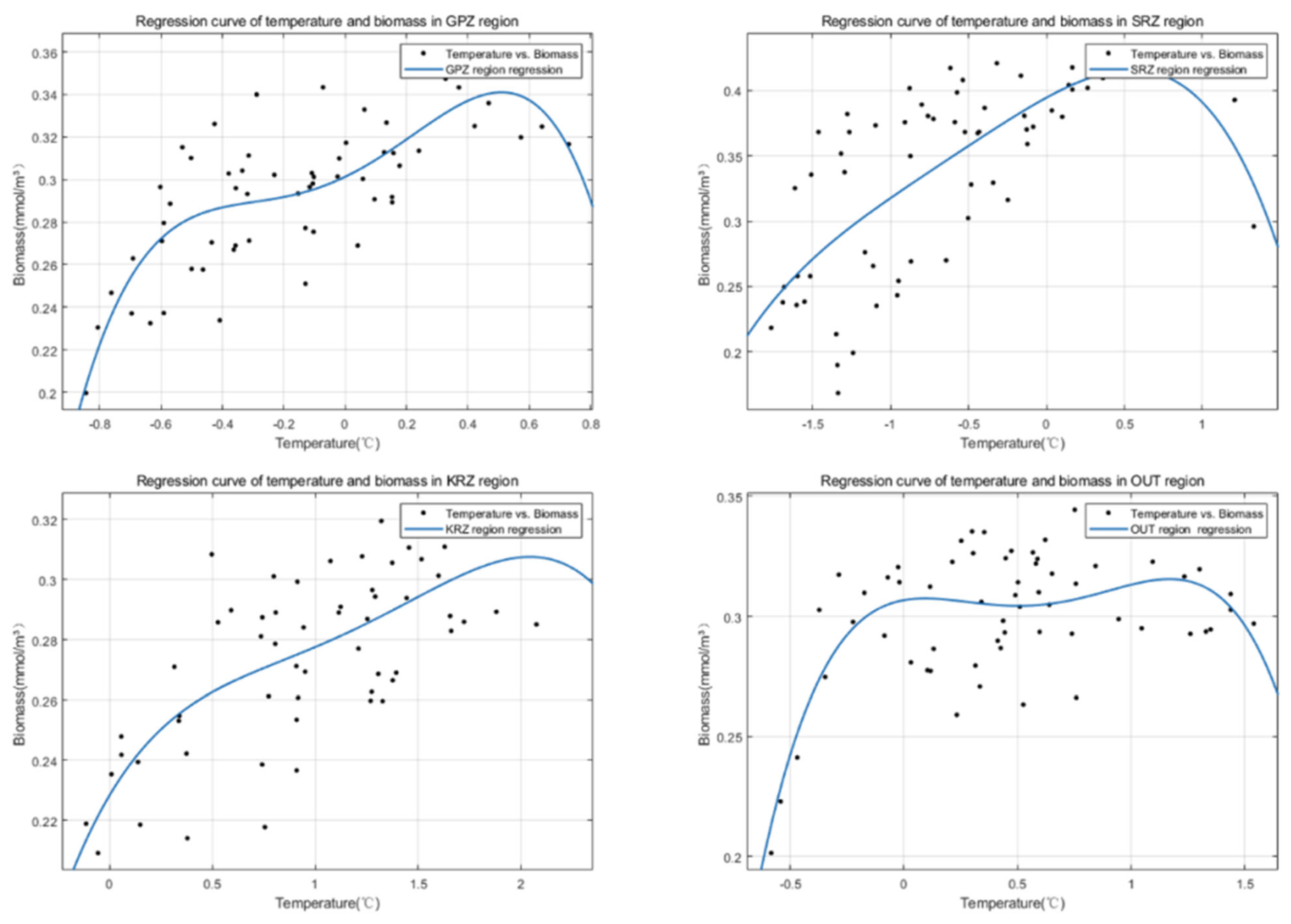
2.3. Study Area Division

Because of the influence of clouds and sea ice, it is difficult to obtain continuous and complete monitoring datasets in the Southern Ocean [33]. This study used a sea ice model to simulate and obtain data on environmental factors and biomass in the Ross Sea. We investigated the relationship between environmental variables and phytoplankton biomass through statistical methods and studied possible regional differences in these variables in the general protection zone, the special research zone, and the krill research zone. The results provide a basis for future protected area management. The first step was to sort the data according to the different areas. We used the areas described in the CCAMLR document, Conservation Measure 91-05 (2016) (Figure 2).

The general protection zone (GPZ) is divided into three areas:

(1)

The area bounded by a line starting where the meridian at 160° E intersects the coastline, thence due north to 65° S, thence due east to 173°45′ E, thence due south to 73°30′ S, thence due east to 180°, thence due south to 76° S, thence due east to 170° W, thence due south to 76°30′ S, thence due east to 164° W, thence due north to 75° S, thence due west to 170° W, thence due north to 72° S, thence due east to 150° W, thence due south to the coastline, and thence along the coastline to the starting point.

(2)

The area bounded by a line starting at 62°30′ S 163° E, thence due north to 60° S, thence due east to 168° E, thence due south to 62°30′ S, and thence due west to the starting point.

(3)

The area bounded by a line starting at 69° S 179° E, thence due north to 66°45′ S, thence due east to 179° W, thence due south to 69° S, and thence due west to the starting point.

The special research zone (SRZ) is bounded by a line starting at 180° 76° S, thence due north to 73°30′ S, thence due east to 170° W, thence due south to 75° S, thence due east to 164° W, thence due south to 76°30′ S, thence due west to 170° W, thence due north to 76° S, and thence due west to the starting point.

The Krill Research Zone (KRZ) is bounded by a line starting where the meridian at 150° E intersects the coastline, thence due north to 62°30′ S, thence due east to 160° E, thence due south to the coastline, and thence along the coastline to the starting point.

2.4. Method

In this study, surface sea ice and environmental factors were compared and analyzed. Monthly averages for different types of marine protected areas were collected from 1958 to 2018, characterizing spring phytoplankton blooms in February. Then, we focus on the data in February and analyze the inter-annual trend in February. We calculated the correlations between biomass and environmental variables in different protected areas and compared their differences. Next, we wanted to understand how phytoplankton biomass and environmental factors would change under future warming scenarios. So, we compared the five hottest years with the average year to find out the differences between them, so as to get a preliminary understanding of which marine protected areas should focus on each variable after the climate warms in the future. Finally, we plotted regression curves for biomass and environmental variables using quartic polynomial fits to find the saturation point of the variable trends. Comparing the sensitivity of different protection zones when the temperature changes show opposite trends. The regression curve is mainly the fitting of phytoplankton and a single environmental variable, and the polynomial function is defined:

$$\widehat{y_i}=a_0{x}_i^n+a_1{x}_i^{n-1}+a_2{x}_i^{n-2}+\cdots +a_{n-1}{x}_i+a_n$$

In order to judge the difference between $\widehat{y_i}$ and the $y_i$ of the sample point, the sum of squares of residuals can be used to represent:

$$ϵ={\displaystyle \sum }_{i=1}^m{\left(\widehat{y_i}-y_i\right)}^2$$

If we can get a set of fitting coefficients that minimizes $ϵ$, then we can say that we have found the best fitting coefficients. Then, we take the partial derivatives of $ϵ$, and we set each of them equal to 0. The coefficients (a₀, a₁, …, a_n) can be obtained by solving the following equations.

$$\left\{\begin{array}{l}\frac{\partial ϵ}{\partial a_0}=0\\ \frac{\partial ϵ}{\partial a_1}=0\\ \hspace{1em}\dots \\ \frac{\partial ϵ}{\partial a_n}=0\end{array}\right.$$

3. Results

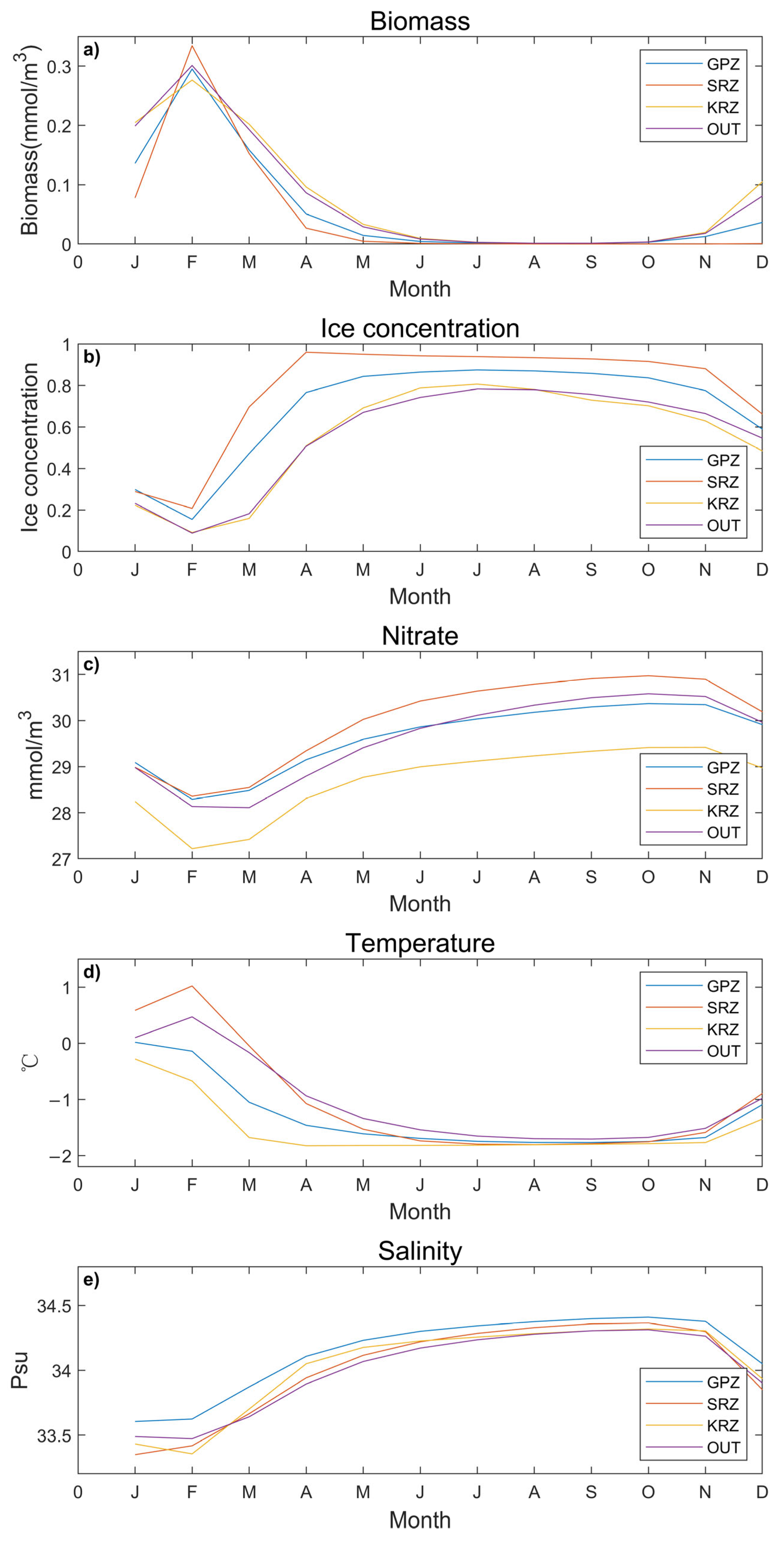
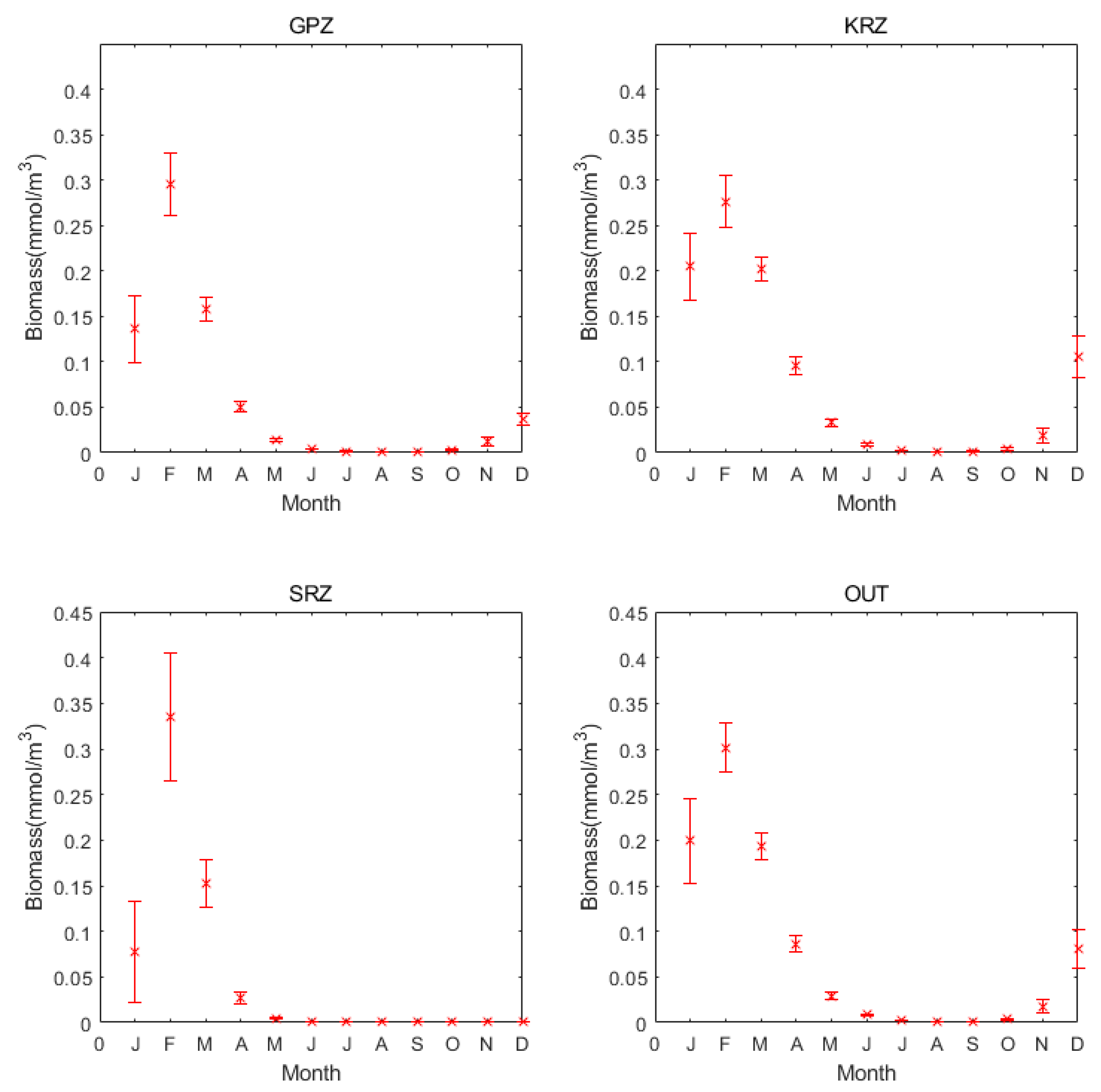
3.1. Annual Cycle Trends of Different MPA in the Ross Sea

The annual cycle trends are similar in each region, but the value is different; the biomass, ice concentration, nitrate, and temperature of the SRZ are higher than for the other regions (Figure 3). Phytoplankton biomass peaks on the sea surface in February, and it is relatively low for most of the year. From March to September, the temperatures are very low but the ice concentrations and the salinity are high. Since the sea surface is covered by sea ice, the biomass during this period is close to zero.

Concerning the other major trends, sea ice concentration is correlated with temperature. These concentrations are high from April to September. The temperatures begin to rise around October, leading to a decrease in sea ice concentration. Sea ice melt causes salinity to decrease. The variations in nitrate concentrations have a similar trend to salinity. We focused on the part of the plot presenting a lag between environmental variables and changes in phytoplankton biomass. Because they are monthly data, hysteresis is not obvious. Although the regions are somewhat different, phytoplankton biomass peaked in February. However, the pulse is short-lived concerning regional variability, the concentration of ice is greater in the KRZ throughout the year compared to the other regions. The concentration of nitrate in the KRZ region is always much lower than in the other areas. Further work is needed to understand the regional differences observed for these environmental variables. In general, these observations are consistent with phytoplankton dynamics growth starting in early spring, which is in September and October, and blooms terminate in March.

The monthly average phytoplankton biomass distribution in the Ross Sea area is shown in Figure 4. These results show that the biomass is very low from May to October. From November, the phytoplankton began to appear in the northernmost part of the Ross Sea and progressively move to the south. It reaches a peak of biomass in February when it covers almost the entire coast of the Ross Sea. In March and April, the phytoplankton gradually disappeared. The data of all years are averaged here, and in the Section 3.5, we will compare them with the data of hot temperature years to observe changes in the distribution and abundance of phytoplankton.

In February, most of the phytoplankton biomass is found close to the southern boundary. However, on the southwest coast of the GPZ region, there is a clear difference, as the biomass there is lower (Figure 5). In addition, there are three locations in the GPZ region, and their distribution is relatively scattered with most of them close to the coastline. The KRZ region is on the westernmost side and spans lower latitudes. The SRZ area is at the southernmost and close to the coast. Therefore, the ice concentration in the SRZ area is higher. Because the phytoplankton bloom tracks from north to south following the receding ice edge, the bloom in the SRZ is relatively short. Most of the SRZ area is on the coast, so the average peak value is higher. The outside region is a more open region. According to the distribution of biomass, it is divided into two regions with an unparallel line (about 66S), with the southern region having higher biomass than the northern one. This may be dominated by latitude and front.

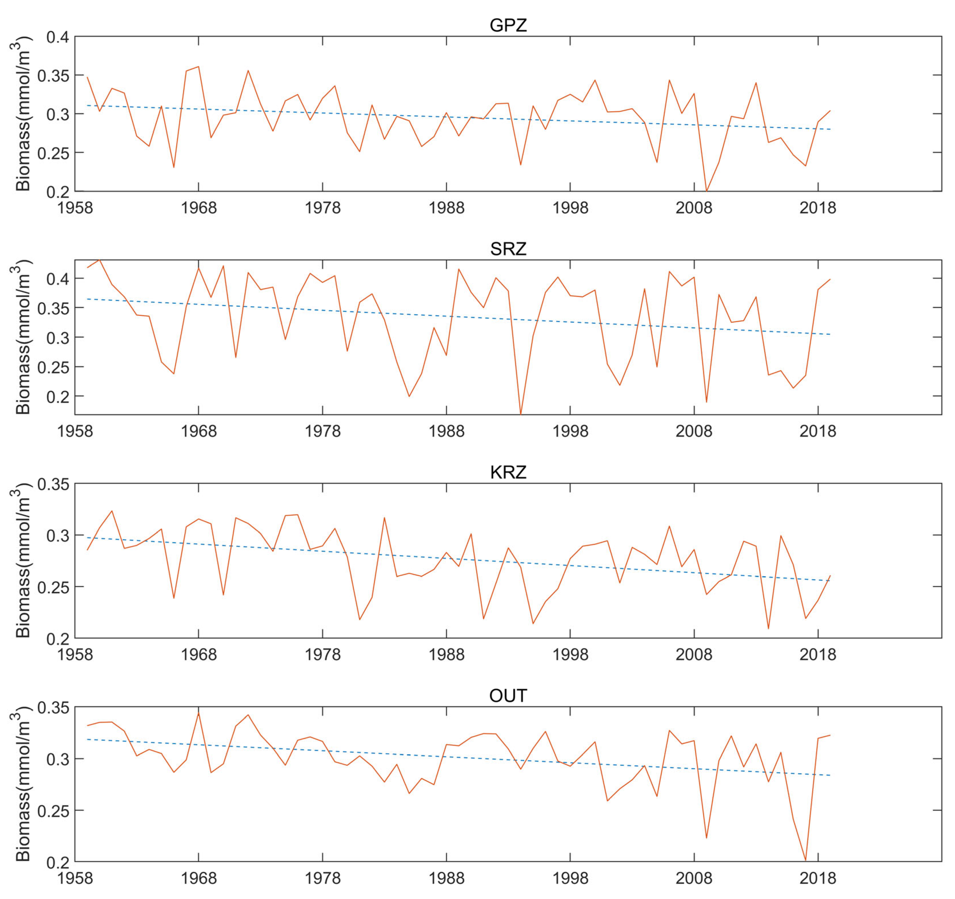
3.2. The Interannual Variation Trend in February

The phytoplankton biomass reached a maximum in February, and the environmental variables seem to change in September. When the winter is over (October), the temperature starts to rise and the sea ice begins to melt. The temperature variations drive the ice concertation, the salinity, and a series of environmental changes. To examine the trend in the dataset concerning the year and the relative abundance of phytoplankton each February (Figure 6). We used a one-variable regression, and the slope of the straight lines are all negative numbers (−5.1218 × 10⁻⁴, −9.9538 × 10⁻⁴, −6.9481 × 10⁻⁴, and −5.7819 × 10⁻⁴), and the R-square values are, respectively, 0.07, 0.06, 0.17, and 0.14. This shows that in each region, the biomass decreases over time. Among them, the SRZ region is the most obvious. Combining the variance (in Figure 7), it is also evident that the SRZ region has relatively pronounced fluctuations. The “outside area” is in the open sea, and the changes are relatively small. The peaks and valleys of biomass appear alternately. Next, to explore what variables are driving biomass. I will do correlation comparisons with environment variables in the next section.

Figure 7 shows the monthly average biomass and the variance for each region. In the SRZ region, average the biomass is the highest, with 0.334 mmol/m³, and has the largest variance of 0.0701. This means that there have been relatively large fluctuations in the SRZ region between the different years. Despite this, it still has higher biomass than the other regions. The GPA and OUT region average biomass of 0.2952 mmol/m³ and 0.3012 mmol/m³, respectively, both close to 0.3 mmol/m³. Additionally, the variances are 0034 and 0.02687. The KRZ region has the lowest average biomass with 0.276 mmol/m³ and a variance of 0.0294.

Figure 8 shows the relationship between temperature and year for the four regions. The trendline slopes in those four different regions are −0.0093, −0.0055, −0.0153, and −0.0102 for the GPZ, SRZ, KRZ, and OUT, respectively, and the R-square values are 0.17, 0.02, 0.23, and 0.12. This suggests that temperatures in the Ross Sea region have been falling over the past few years, and at SRZ, the decades-long drop in sea surface temperatures is less pronounced.

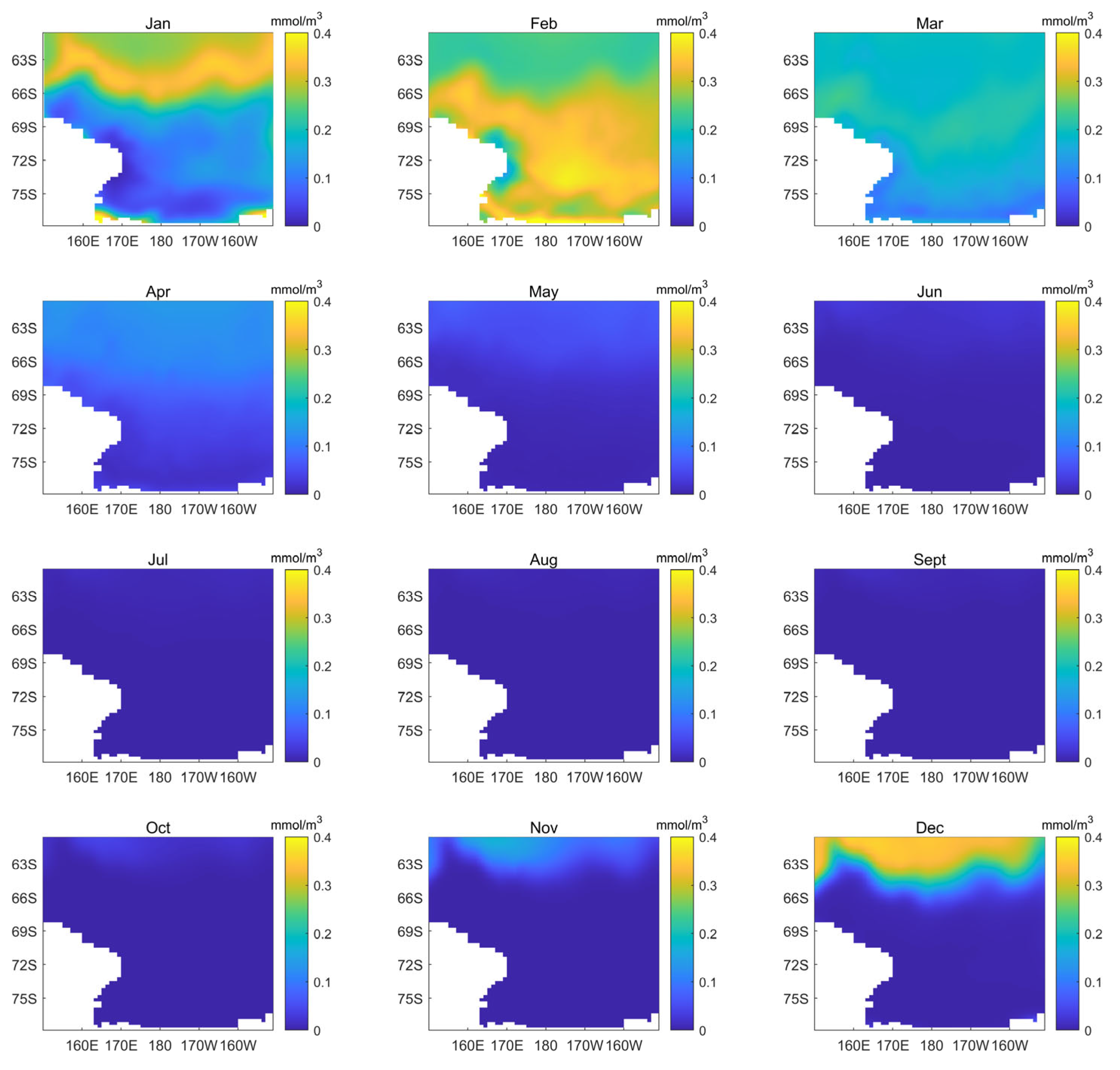
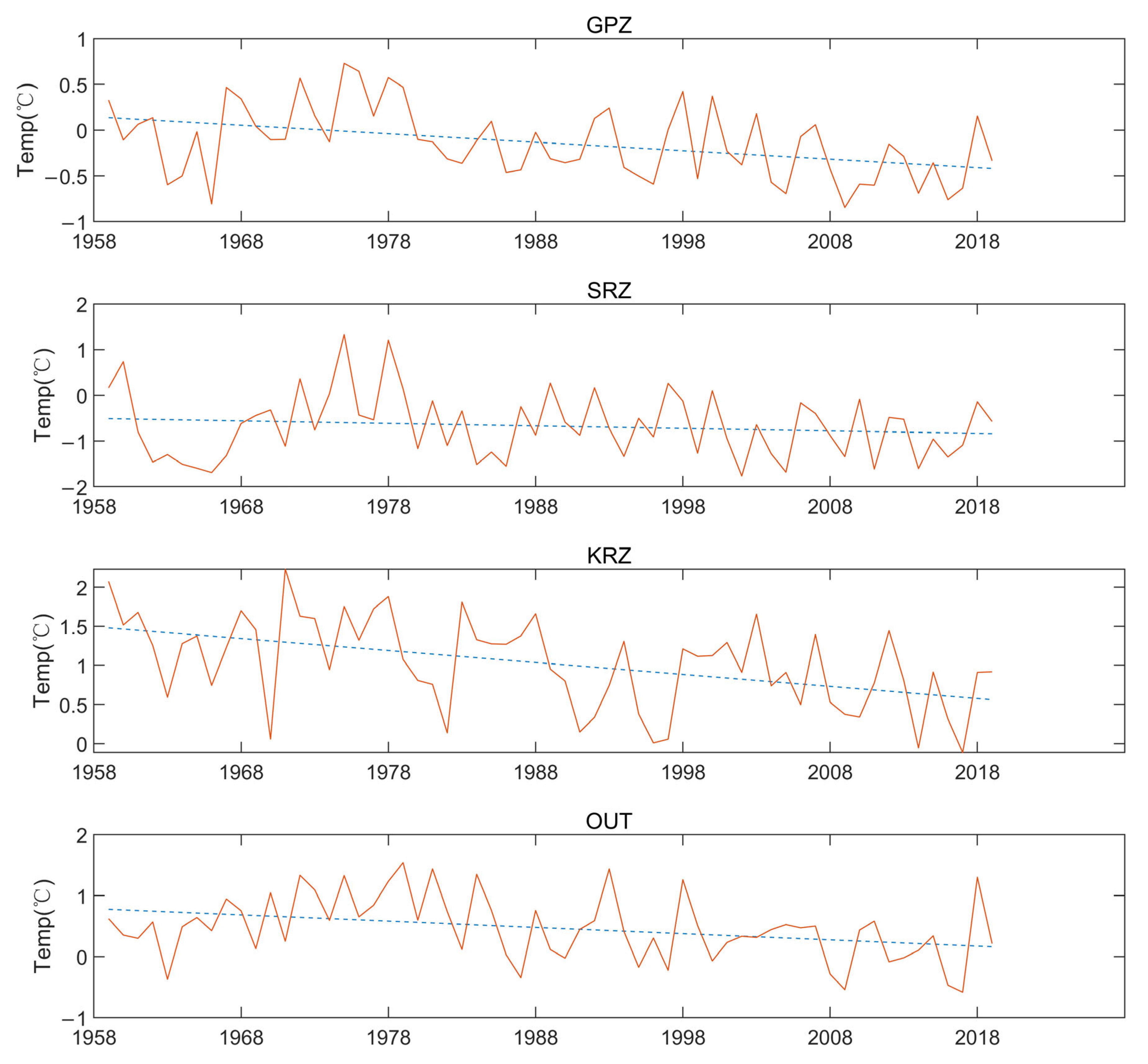
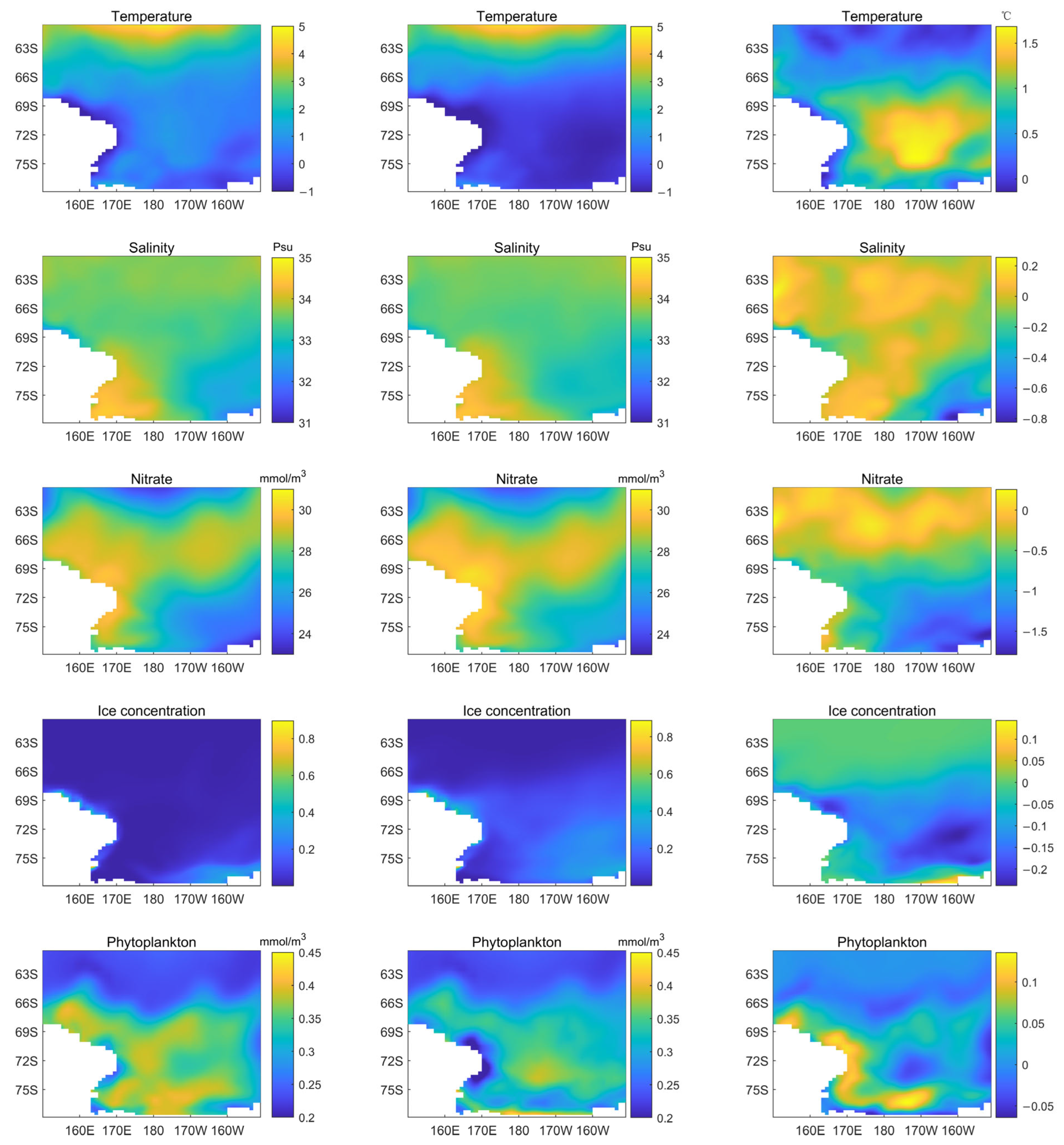
3.3. Spatial Variability in Phytoplankton Biomass and Other Environmental Variables in the Ross Sea

To determine the spatial relationship between phytoplankton abundance in February and four key environmental variables, correlation coefficients were used to assess the significance of all four regions.

The positive coefficient between biomass and temperature is over 0.6 in the three MAP regions, but the outside region is only 0.3829. The relationship between biomass and salinity is weak within the MPA, but there is a moderate negative relationship outside the MPA, about −0.4074. Biomass and sea ice were moderately negatively correlated both within and outside the MPA. We observed a negative correlation between biomass and nitrate levels for three regions suggesting that increased growth levels were due to a reduction in nitrate availability. In summary, the relationship between salinity and biomass is not significant within the MPA. Temperature (positive), sea ice concentration (negative), and nitrate concentrations (negative), in contrast, all have a high correlation with biomass.

3.4. Lag Correlation Analysis

Because the environmental variables in this system are dynamic, there is likely to be a lag in environmental forcing. Therefore, we also explored the relationship between environmental variables in January and biomass in February. The correlations between biomass, temperature, and ice are similar to those shown in

Table 2. Correlation coefficients of phytoplankton biomass and other environmental variables in different MPA regions and outside in February.

	Temperature		Salinity		Ice		Nitrate
	r	p-Value	r	p-Value	r	p-Value	r	p-Value
GPZ	0.723	0.000	−0.217	0.093	−0.534	0.000	−0.553	0.000
SRZ	0.607	0.000	−0.210	0.105	−0.578	0.000	−0.541	0.000
KRZ	0.711	0.000	0.156	0.230	−0.590	0.000	−0.168	0.196
OUT	0.383	0.002	−0.407	0.001	−0.539	0.000	−0.405	0.001

. In three MP regions, the correlation between biomass and sea ice in January was even greater than that in February (Table 2 and

Table 3. Correlation coefficients of phytoplankton biomass (February) and other environmental variables (January) in different MPA regions and outside in February.

	Temperature		Salinity		Ice		Nitrate
	r	p-Value	r	p-Value	r	p-Value	r	p-Value
GPZ	0.639	0.000	−0.439	0.000	−0.586	0.000	−0.332	0.009
SRZ	0.485	0.000	−0.345	0.006	−0.582	0.000	−0.243	0.059
KRZ	0.651	0.000	−0.057	0.661	−0.713	0.000	−0.010	0.940
OUT	0.299	0.020	−0.536	0.000	−0.419	0.000	−0.238	0.065

). The salinity showed a strong negative correlation. The negative correlation of nitrate was smaller. However, the KRZ region is different from other regions. The coefficient becomes very small. Hence, in January, some variables still had a strong correlation, so those variables could provide some evidence for the forecast.

3.5. Years with Unusually High Temperatures

To explore unusual temperature trends in the dataset, we picked the five warmest February months of all available years and compared the averages. On the left side of Figure 9 is the average of the five warmest Februarys, in the middle is the average of Februarys over the calendar years, and on the right is the difference between them. The temperature difference is mainly distributed in the southeast Ross Sea, SRZ region, and some GPZ regions. The same observation can be made for salinity. The southwest corner of the Ross Sea has higher salinity. Nitrate distribution is very similar. Nitrate concentrations typically fall during the warmest years. Nitrate differences are concentrated in the northern Ross Sea, and their distribution appears to vary with latitude. Since February is the hottest month in Antarctica, sea surface temperatures are generally above freezing and the ice concentration is almost zero. On average, only a small amount of ice exists in the Northeast each year. In the warmest years, phytoplankton biomass increases, with significant increases in coastal areas. Notably, phytoplankton biomass increased significantly in the SRZ and GPZ regions but remained low in the southeast.

In general, as the temperature rises, the biomass in different regions increases (Figure 10). The basic quartic polynomial fitting function is defined as $\widehat{y_i}=a_0{x}_i^4+a_1{x}_i^3+a_2{x}_i^2+a_3{x}_i+a_4$. This trend confirms the results observed in Figure 9 and is consistent with the positive correlations obtained in the third and fourth parts of the results. However, the temperature sensitivity is not the same according to the region considered. The KRZ area reaches the peak of the biomass at 2 degrees centigrade. The maximum value of biomass in the SRZ region is the largest, which is consistent with the results shown in Figure 7. Although subtle, there is a trend whereby biomass begins to decline as the temperature increases.

4. Discussion

4.1. Limitation and Plan

The physical model in this research is the Australian Community Climate and Earth-System Simulator, ACCESS-OM2. It has three resolutions in total: a coarse resolution (nominally 1° horizontal grid spacing), an eddy-permitting resolution (nominally 0.25°), and an eddy-rich resolution (0.1° with 75 vertical levels). The eddy-rich model is designed to be incorporated into the Bluelink 5 operational ocean prediction and reanalysis system. All resolutions have their advantages and disadvantages. For instance, in Kiss’s study, they found that for the analysis of the small straits, the structure of western boundary currents, and the 10 abyssal overturning cells, higher resolution is better than lower. However, there is still scope for improvement in sub-grid scale parameterization at the highest resolution [26]. Our output is eddy-permitting resolution (0.25°). Compared with the coarse resolution (1° horizontal grid spacing), the 1° model does not resolve the ocean mesoscale [34]. That means that it ignores the key processes that can influence the climate. Higher resolution usually has better estimates of vertical heat transport, enhancement of boundary currents, better resolution of ocean straits, and improved Southern Ocean state by improving the climate state [34,35,36].

The biogeochemical (BGC) cycles model is the whole ocean model with biogeochemistry and trophic-dynamics (WOMBAT). It simulates five state variables representative of the low-trophic level of the ecosystem: nitrate, iron, phytoplankton, zooplankton, and detritus. The growth rate of phytoplankton depends on temperature, light, nitrate, and iron. The temperature determines the maximum specific growth rate, following the Eppley curve [37], whereas reduced light or nutrient concentrations can limit the growth rate, as displayed in the Monod equation [38]. Although iron can be limiting for phytoplankton growth, the preliminary analysis in the Hayashida paper indicates that it is never limiting in the model simulation [39]. So, in our research, we excluded iron from the analysis and added ice concentration instead of the light limitation. The simulated and observed findings apply to the whole phytoplankton community, but the responses of different functional types and size classes of phytoplankton are presumably variable because the growth rates changed according to temperature, light, and nutrient conditions [39]. The NPZD model is a simple model to help us describe the results and functions of the ecosystem in detail by reproducing the flow of energy in the low trophic levels of the food web. So, in the BGC model, we ignored the limitation of other macro and micro-nutrients. These considerations should not change the conclusion about the general relationship between phytoplankton bloom and nutrient concentration. Our research next step could be to use a more complex ocean biogeochemistry model to analyze these topics.

4.2. Lack of Perceived Temperature Change in the Ross Sea

In the last decades, there have been few signs of climate warming in the Southern Ocean, in sharp contrast with the rapid warming observed in the Arctic. However, along the northern side of the Antarctic Circumpolar Current, the upper ocean has warmed significantly [40]. Armour et al. showed through ocean observations and simulation of atmospheric circulation patterns that the delayed warming south of the Antarctic circumpolar current and the enhanced warming of the Arctic are caused by the meridional overturning circulation in the Southern Ocean: wind-driven upwelling of unmodified water from depth damps warming around Antarctica; greenhouse gas-induced surface heat uptake is largely balanced by anomalous northward heat transport associated with the equatorward flow of surface waters; and heat is preferentially stored where surface waters are subducted to the north.

Since the formation of sea ice is the result of ocean-atmospheric heat, freshwater, and momentum exchanges, it integrates the elements of the ocean and atmospheric circulation. Thermodynamically, the sea ice processes may have a role in modulating the exposure of Antarctic ice shelves to warm circumpolar deep water [41,42,43] and in changing the temperature and salinity properties of that water, which may also affect basal melt [44]. These environmental changes may drive changes in phytoplankton biomass/community. The current research on Antarctic sea ice is still challenging, and the deviation of sea ice creates great uncertainty in the prediction of future climate change in Antarctica [45,46]. It is very important to understand these changes and the broader issue of climate change [47].

Under this special temperature trend, the results of our model are also inconsistent with global warming. There is even a downward trend. We need to keep monitoring environmental changes and model outputs for comparison. At the same time, the extent of Antarctic sea ice has also increased. It is characterized by huge regional differences and interdecadal changes. In the Ross Sea, 50% of the sea ice is produced within wind-sustained latent-heat polynyas [48]. In this study, phytoplankton biomass and sea ice are negatively correlated. In Mezgec’s study, combined information from marine diatom records and sea salt sodium and water isotope ice core records showed an increase in the efficiency of regional latent-heat polynyas which resulted in more coastal sea ice. These past changes are consistent with a significant decrease in the number of penguins, whitebaits, and seals. Due to the relationship between primary productivity and their food web, there may also be a connection. The distribution and quantity of marine organisms may be related to the distribution of phytoplankton communities. To figure this out, we need to simulate more complex biological models in the future. However, this can confirm the high sensitivity of marine ecosystems to the environment, especially coastal sea ice conditions.

4.3. Changes in Sea Ice in the Southern Ocean and Ecological Impacts, Interactions in the Ecosystem of the Ross Sea Shelf

Although Antarctic sea ice has increased slightly overall, its temporal and spatial characteristics (especially its seasonality) are undergoing major regional changes [48]. In Mezgec’s study, they assessed the significance of Antarctic sea ice to biology, emphasizing the importance of scale, thermodynamics, and dynamics. The change in sea ice cover has a direct and indirect impact on the structure and function of the ecosystem. Changes in ice caves and fixed ice can favor the emergence of extreme events such as increased storminess/waviness, the number of icebergs, and snowfall [49]. Storms also led to a convergence in the sea ice motion, which causes rapid dynamic thickening of the existing ice by rafting and pressure ridge formation. These extreme events will affect the ice in a short time, thereby affecting the phytoplankton as well. The pack ice is an important habitat for krill and the survival of larval krill [50].

Seasonal pack ice dynamics will affect krill population dynamics. The timing of sea ice retreat influences the timing of food availability for female Antarctic krill and thus ovarian development in spring; whereas the timing of sea ice advance is linked to juvenile survival and recruitment success (in the Palmer LTER region) [51]. In the vast continental shelf ecosystem of the Ross Sea, krill play an important role in the food web [7]. In the Ross Sea MPA, a krill region has also been specially set up. This protected area is suitable to study krill behavior and community dynamics. To understand the entire ecosystem, it is essential to study the low trophic level of primary producers and krill. Combined with the results of our research, the KRZ area is worthy of attention. The correlation between biomass and nitrate is not strong in this KRZ region, compared to the other regions. For the lag correlation analysis, the correlation between biomass and salinity increased overall. However, the KRZ region declined. This may be related to the terrain and the biological influence of krill, but it is still unknown at this moment.

4.4. The Future of the Ross Sea MPA Research

In history, seals and whales in the Ross Sea have encountered some exploitation, and recently the area has become the target of tourism, scientific research, and commercial fishing (Antarctic toothfish). When we lack monitoring and research on the ecosystem in the region, it is worrying that such things happen. The establishment of marine protected areas in the future is necessary. The establishment of marine protected areas aims to protect and manage the ecosystems they delimit, while reasonably developing natural and cultural resources [2].

Future research on the Ross Sea MPA is very broad but challenging. To achieve reasonable development, scientific evaluation is needed. This requires research results based on the Antarctic climate, ocean circulation, and sea ice changes. We need to get more accurate model outputs and more convincing triggering explanations to support the research of biological systems. In this study, the NPZD model was used to simulate the changes in phytoplankton biomass and community using a simple nitrogen cycle. This is a good start. In the future, more complex ocean ecological models should be built. We hope that research on the Ross Sea MPA will help to better manage and protect the entire Antarctic ecosystem in the future.

The Commission for the Conservation of Antarctic Marine Living Resources (CCAMLR), as the organization responsible for the management of living natural resources in the Southern Ocean, needs projections of primary productivity, Antarctic biology, and ecosystems based on likely future changes in climate. This study is a first attempt at providing that information so that CCAMLR can make informed decisions regarding the maximum protection of endangered species and so avoid irreversible changes in marine ecology.

5. Conclusions

Research solved the three initial goals: the relationship between environmental variables and phytoplankton biomass in the Ross Sea area. The relationship between salinity and biomass is not significant but temperature (positive), sea ice concentration (negative), and nitrate concentrations (negative) in contrast, all have a high correlation with biomass and also explored hysteresis. Depending on the correlation coefficient support, we can potentially forecast conditions in February one or two months earlier. This provides a reference for future research. However, the KRZ region is special, the correlation coefficient of salinity and nitrate is different from other regions. We need to do further research to know why happened. Because of the limitations of the model, we did not compare and evaluate the results generated for different resolutions. This needs to be compared with satellite data to be evaluated. Different regions may be suitable for different resolutions. This is the work that needs to be carried out in the future. The exploration of space abnormality is not extensive, and it is necessary to combine satellite observations and ocean phenomena to better explain the reasons. We also made predictions on future changes in phytoplankton biomass, according to the regression curve, a short period of temperature rise may lead to an increase in phytoplankton biomass. However, for long time series, the future trend of phytoplankton biomass is still full of uncertainty. Based on other papers, the prediction of sea ice has great uncertainty for future climate changes. Sea ice affects the occurrence of extreme events and the structure and function of biological systems. In terms of thermodynamics and kinetics, the prediction of sea ice is challenging. In addition, the time interval of the model output is very large, which is not suitable for the analysis of the relationship between variables. We need to run the model longer to get more results. For the study of the Ross Sea ecosystem, we need more advanced sea ice models and more complex biological models, which consider the regional differences. Once we have completed these goals, I believe this will be of great significance for the study of the entire Antarctic ecosystem. In this way, we can better protect Antarctic life and protect, utilize, and develop Antarctic resources.

References

1. Waterhouse, E.J. (Ed.) Ross Sea Region 2001: A State of the Environment Report for the Ross Sea Region of Antarctica; New Zealand Antarctic Inst.: Christchurch, New Zealand, 2001. [Google Scholar]
2. Beer, K.; Brears, R.; Briars, L.; Roldan, G. A Pragmatic Utopia: Should the Ross Sea be Designated a Marine Protected Area? University of Canterbury: Christchurch, New Zealand, 2011. [Google Scholar]
3. Silvano, A.; Foppert, A.; Rintoul, S.R.; Holland, P.R.; Tamura, T.; Kimura, N.; Macdonald, A.M. Recent recovery of Antarctic Bottom Water formation in the Ross Sea driven by climate anomalies. Nat. Geosci. 2020, 13, 780–786. [Google Scholar] [CrossRef]
4. Castagno, P.; Capozzi, V.; DiTullio, G.R.; Falco, P.; Fusco, G.; Rintoul, S.R.; Budillon, G. Rebound of shelf water salinity in the Ross Sea. Nat. Commun. 2019, 10, 5441. [Google Scholar] [CrossRef] [PubMed] [Green Version]
5. Brooks, C.M.; Bloom, E.; Kavanagh, A.; Nocito, E.S.; Watters, G.M.; Weller, J. The Ross Sea, Antarctica: A highly protected MPA in international waters. Mar. Policy 2021, 134, 104795. [Google Scholar] [CrossRef]
6. Eastman, J.T. The nature of the diversity of Antarctic fishes. Polar Biol. 2005, 28, 93–107. [Google Scholar] [CrossRef]
7. Smith, W.O., Jr.; Ainley, D.G.; Cattaneo-Vietti, R. Trophic interactions within the Ross Sea continental shelf ecosystem. Philos. Trans. R. Soc. B Biol. Sci. 2007, 362, 95–111. [Google Scholar] [CrossRef] [PubMed]
8. Schine, C.M.; van Dijken, G.; Arrigo, K.R. Spatial analysis of trends in primary production and relationship with large-scale climate variability in the Ross Sea, Antarctica (1997–2013). J. Geophys. Res. Ocean. 2016, 121, 368–386. [Google Scholar] [CrossRef] [Green Version]
9. Parkinson, C.L.; Cavalieri, D.J. Antarctic sea ice variability and trends, 1979–2010. Cryosphere 2012, 6, 871–880. [Google Scholar] [CrossRef] [Green Version]
10. Cavalieri, D.J.; Parkinson, C.L.; Gloersen, P.; Comiso, J.C.; Zwally, H.J. Deriving long-term time series of sea ice cover from satellite passive-microwave multisensor data sets. J. Geophys. Res. Ocean. 1999, 104, 15803–15814. [Google Scholar] [CrossRef]
11. Hobbs, W.R.; Massom, R.; Stammerjohn, S.; Reid, P.; Williams, G.; Meier, W. A review of recent changes in Southern Ocean sea ice, their drivers and forcings. Glob. Planet. Chang. 2016, 143, 228–250. [Google Scholar] [CrossRef] [Green Version]
12. Deppeler, S.L.; Davidson, A.T. Southern Ocean phytoplankton in a changing climate. Front. Mar. Sci. 2017, 4, 40. [Google Scholar] [CrossRef] [Green Version]
13. Hückstädt, L.A.; Piñones, A.; Palacios, D.M.; McDonald, B.I.; Dinniman, M.S.; Hofmann, E.E.; Costa, D.P. Projected shifts in the foraging habitat of crabeater seals along the Antarctic Peninsula. Nat. Clim. Chang. 2020, 10, 472–477. [Google Scholar] [CrossRef]
14. Mitchell, B.G.; Brody, E.A.; Holm-Hansen, O.; McClain, C.; Bishop, J. Light limitation of phytoplankton biomass and macronutrient utilization in the Southern Ocean. Limnol. Oceanogr. 1991, 36, 1662–1677. [Google Scholar] [CrossRef]
15. Martin, J.H.; Fitzwater, S.E.; Gordon, R.M. Iron deficiency limits phytoplankton growth in Antarctic waters. Glob. Biogeochem. Cycles 1990, 4, 5–12. [Google Scholar] [CrossRef] [Green Version]
16. Charlson, R.J.; Lovelock, J.E.; Andreae, M.O.; Warren, S.G. Oceanic phytoplankton, atmospheric sulphur, cloud albedo and climate. Nature 1987, 326, 655–661. [Google Scholar] [CrossRef]
17. Meiners, K.M.; Vancoppenolle, M.; Thanassekos, S.; Dieckmann, G.S.; Thomas, D.N.; Tison, J.L.; Raymond, B. Chlorophyll a in Antarctic sea ice from historical ice core data. Geophys. Res. Lett. 2012, 39, L21602. [Google Scholar] [CrossRef]
18. Miller, C.B. Biological Oceanography; John Wiley & Sons: Hoboken, NJ, USA, 2009. [Google Scholar]
19. Smith, W.O.; Nelson, D.M. Phytoplankton bloom produced by a receding ice edge in the Ross Sea: Spatial coherence with the density field. Science 1985, 227, 163–166. [Google Scholar] [CrossRef] [PubMed]
20. Lizotte, M.P. The contributions of sea ice algae to Antarctic marine primary production. Am. Zool. 2001, 41, 57–73. [Google Scholar] [CrossRef]
21. Smith, W.O., Jr.; Nelson, D.M.; DiTullio, G.R.; Leventer, A.R. Temporal and spatial patterns in the Ross Sea: Phytoplankton biomass, elemental composition, productivity and growth rates. J. Geophys. Res. Ocean. 1996, 101, 18455–18465. [Google Scholar] [CrossRef]
22. Boyd, P.W.; Arrigo, K.R.; Strzepek, R.; Van Dijken, G.L. Mapping phytoplankton iron utilization: Insights into Southern Ocean supply mechanisms. J. Geophys. Res. Ocean. 2012, 117, C06009. [Google Scholar] [CrossRef] [Green Version]
23. Strzepek, R.F.; Maldonado, M.T.; Hunter, K.A.; Frew, R.D.; Boyd, P.W. Adaptive strategies by Southern Ocean phytoplankton to lessen iron limitation: Uptake of organically complexed iron and reduced cellular iron requirements. Limnol. Oceanogr. 2011, 56, 1983–2002. [Google Scholar] [CrossRef] [Green Version]
24. De Baar, H.J.; de Jong, J.T.; Bakker, D.C.; Löscher, B.M.; Veth, C.; Bathmann, U.; Smetacek, V. Importance of iron for plankton blooms and carbon dioxide drawdown in the Southern Ocean. Nature 1995, 373, 412–415. [Google Scholar] [CrossRef]
25. Sohrin, Y.; Iwamoto, S.I.; Matsui, M.; Obata, H.; Nakayama, E.; Suzuki, K.; Ishii, M. The distribution of Fe in the Australian sector of the Southern Ocean. Deep Sea Res. Part I Oceanogr. Res. Pap. 2000, 47, 55–84. [Google Scholar] [CrossRef]
26. Kiss, A.E.; Hogg, A.M.; Hannah, N.; Boeira Dias, F.; Brassington, G.B.; Chamberlain, M.A.; Chapman, C.; Dobrohotoff, P.; Domingues, C.M.; Duran, E.R.; et al. ACCESS-OM2 v1.0: A global ocean–sea ice model at three resolutions. Geosci. Model Dev. 2020, 13, 401–442. [Google Scholar]
27. Schiller, A.; Oke, P.R. BLUElink> Development of operational oceanography and servicing in Australia. J. Res. Pract. Inf. Technol. 2007, 39, 151–164. [Google Scholar]
28. Kidston, M.; Matear, R.; Baird, M.E. Parameter optimisation of a marine ecosystem model at two contrasting stations in the Sub-Antarctic Zone. Deep. Sea Res. Part II Top. Stud. Oceanogr. 2011, 58, 2301–2315. [Google Scholar] [CrossRef]
29. Oke, P.R.; Griffin, D.A.; Schiller, A.; Matear, R.J.; Fiedler, R.; Mansbridge, J.; Ridgway, K. Evaluation of a near-global eddy-resolving ocean model. Geosci. Model Dev. 2013, 6, 591–615. [Google Scholar] [CrossRef] [Green Version]
30. Heinle, A.; Slawig, T. Internal dynamics of NPZD type ecosystem models. Ecol. Model. 2013, 254, 33–42. [Google Scholar] [CrossRef]
31. Xue, P.; Schwab, D.J.; Zhou, X.; Huang, C.; Kibler, R.; Ye, X. A hybrid lagrangian–eulerian particle model for ecosystem simulation. J. Mar. Sci. Eng. 2018, 6, 109. [Google Scholar] [CrossRef] [Green Version]
32. Oschlies, A.; Garçon, V. An eddy-permitting coupled physical-biological model of the North Atlantic: 1. Sensitivity to advection numerics and mixed layer physics. Glob. Biogeochem. Cycles 1999, 13, 135–160. [Google Scholar] [CrossRef] [Green Version]
33. Smith, W.O., Jr.; Marra, J.; Hiscock, M.R.; Barber, R.T. The seasonal cycle of phytoplankton biomass and primary productivity in the Ross Sea, Antarctica. Deep Sea Res. Part II Top. Stud. Oceanogr. 2000, 47, 3119–3140. [Google Scholar] [CrossRef]
34. Griffies, S.M.; Winton, M.; Anderson, W.G.; Benson, R.; Delworth, T.L.; Dufour, C.O.; Zhang, R. Impacts on ocean heat from transient mesoscale eddies in a hierarchy of climate models. J. Clim. 2015, 28, 952–977. [Google Scholar] [CrossRef] [Green Version]
35. Hewitt, H.T.; Roberts, M.J.; Hyder, P.; Graham, T.; Rae, J.; Belcher, S.E.; Wood, R.A. The impact of resolving the Rossby radius at mid-latitudes in the ocean: Results from a high-resolution version of the Met Office GC2 coupled model. Geosci. Model Dev. 2016, 9, 3655–3670. [Google Scholar] [CrossRef] [Green Version]
36. Bishop, S.P.; Gent, P.R.; Bryan, F.O.; Thompson, A.F.; Long, M.C.; Abernathey, R. Southern Ocean overturning compensation in an eddy-resolving climate simulation. J. Phys. Oceanogr. 2016, 46, 1575–1592. [Google Scholar] [CrossRef]
37. Eppley, R.W. Temperature and phytoplankton growth in the sea. Fish. Bull 1972, 70, 1063–1085. [Google Scholar]
38. Monod, J. The growth of bacterial cultures. Annu. Rev. Microbiol. 1949, 3, 371–394. [Google Scholar] [CrossRef] [Green Version]
39. Hayashida, H.; Matear, R.J.; Strutton, P.G. Background nutrient concentration determines phytoplankton bloom response to marine heatwaves. Glob. Chang. Biol. 2020, 26, 4800–4811. [Google Scholar] [CrossRef]
40. Armour, K.C.; Marshall, J.; Scott, J.R.; Donohoe, A.; Newsom, E.R. Southern Ocean warming delayed by circumpolar upwelling and equatorward transport. Nat. Geosci. 2016, 9, 549–554. [Google Scholar] [CrossRef]
41. Convey, P.; Bindschadler, R.; di Prisco, G.; Fahrbach, E.; Gutt, J.; Hodgson, D.; Mayewski, P.; Summerhayes, C.; Turner, J. Antarctic climate change and the environment. Antarct. Sci. 2009, 21, 541–563. [Google Scholar] [CrossRef] [Green Version]
42. Holland, P.R.; Jenkins, A.; Holland, D.M. Ice and ocean processes in the Bellingshausen Sea, Antarctica. J. Geophys. Res. Ocean. 2010, 115, C05020. [Google Scholar] [CrossRef] [Green Version]
43. St-Laurent, P.; Klinck, J.M.; Dinniman, M.S. Impact of local winter cooling on the melt of Pine Island Glacier, Antarctica. J. Geophys. Res. Ocean. 2015, 120, 6718–6732. [Google Scholar] [CrossRef] [Green Version]
44. Dutrieux, P.; De Rydt, J.; Jenkins, A.; Holland, P.R.; Ha, H.K.; Lee, S.H.; Schröder, M. Strong sensitivity of Pine Island ice-shelf melting to climatic variability. Science 2014, 343, 174–178. [Google Scholar] [CrossRef] [Green Version]
45. Agosta, C.; Fettweis, X.; Datta, R. Evaluation of the CMIP5 models with the aim of regional modelling of the Antarctic surface mass balance. Cryosphere 2015, 9, 2311–2321. [Google Scholar] [CrossRef] [Green Version]
46. Bracegirdle, T.J.; Stephenson, D.B.; Turner, J.; Phillips, T. The importance of sea ice area biases in 21st century multimodel projections of Antarctic temperature and precipitation. Geophys. Res. Lett. 2015, 42, 10–832. [Google Scholar] [CrossRef] [Green Version]
47. Kennicutt, M.C.; Chown, S.L.; Cassano, J.J.; Liggett, D.; Peck, L.S.; Massom, R.; Sutherland, W.J. A roadmap for Antarctic and Southern Ocean science for the next two decades and beyond. Antarct. Sci. 2015, 27, 3–18. [Google Scholar] [CrossRef] [Green Version]
48. Mezgec, K.; Stenni, B.; Crosta, X.; Masson-Delmotte, V.; Baroni, C.; Braida, M.; Frezzotti, M. Holocene sea ice variability driven by wind and polynya efficiency in the Ross Sea. Nat. Commun. 2017, 8, 1334. [Google Scholar] [CrossRef] [PubMed] [Green Version]
49. Massom, R.A.; Stammerjohn, S.E. Antarctic sea ice change and variability–physical and ecological implications. Polar Sci. 2010, 4, 149–186. [Google Scholar] [CrossRef] [Green Version]
50. Frazer, T.K.; Quetin, L.B.; Ross, R.M. Energetic demands of larval krill, Euphausia superba, in winter. J. Exp. Mar. Biol. Ecol. 2002, 277, 157–171. [Google Scholar] [CrossRef]
51. Quetin, L.B.; Ross, R.M. Life under Antarctic pack ice: A krill perspective. In Smithsonian at the Poles: Contributions to International Polar Year Science; Smithsonian Institution Scholarly Press: Washington, DC, USA, 2009. [Google Scholar]
Figure 1. Diagram of the NPZD model. adapted with permission from Ref. [31]. Xue et al., 2018, Journal of Marine Science and Engineering.
Jmse 11 00747 g001
Figure 2. Map of the Ross Sea marine protected area (Source: https://www.mfat.govt.nz/en/environment/antarctica-and-the-southern-ocean/ross-sea-region-marine-protected-area/ (accessed on 8 March 2023)).
Jmse 11 00747 g002
Figure 3. Monthly time-series of the different variables for the four different regions from 1958 to 2018: (a) Biomass (b) ice concentration; (c) nitrate; (d) temperature; (e) salinity (three type of the MPA region and one outside).
Jmse 11 00747 g003
Figure 4. Map of monthly average phytoplankton biomass (mmol/m3) in the Ross Sea region from 1958 to 2018.
Jmse 11 00747 g004
Figure 5. Average biomass in the Ross Sea area in February from 1958 to 2018 and location of the marine protected areas (dotted line).
Jmse 11 00747 g005
Figure 6. Annual variation of biomass in February in the different MPA regions.
Jmse 11 00747 g006
Figure 7. Monthly average biomass and variance of the different regions from 1958 to 2018.
Jmse 11 00747 g007
Figure 8. Annual variations of temperature in February in the different MPA regions.
Jmse 11 00747 g008
Figure 9. Map distribution of the different environmental variables’ concentration in February: (1) an average of the five warmest years (left), (2) an average of all the years (middle), and (3) the difference between them (right). Note: the concentration range of the color bars is different.
Jmse 11 00747 g009
Figure 10. Regression curves of temperature vs. biomass in four MPA regions. (Polynomial function with 4 degrees).
Jmse 11 00747 g010