Nonparametric Identification Model of Coupled Heave–Pitch Motion for Ships by Using the Measured Responses at Sea

Abstract

In order to simulate or control the coupled heave–pitch motion of ships in waves as realistically as possible, an appropriate mathematical model must be established in advance. In this paper, a nonparametric identification method, based on a combination of a random decrement technique (RDT) and support vector regression (SVR), was proposed to model the coupled heave–pitch motion of ships by only using the measured random responses at sea. First, a mathematical model was established to describe the coupled heave–pitch motion of ships in irregular waves. Second, the random decrement equation and the random decrement signatures were obtained by using RDT. Third, the damped frequency of the coupled heave–pitch motions were obtained by analyzing the random decrement signatures. Fourth, SVR was applied to identify the unknown hydrodynamic functions in the established mathematical model. The applicability and validity of the proposed nonparametric identification method were verified by case studies which were designed based on the simulated data and the model test data, respectively. Results of the study showed that the nonparametric identification method can be applied to identify the coupled heave–pitch motion of ships by only using the measured random responses in irregular waves.

1. Introduction

Nowadays, with the rapid development of intelligent ships, motion simulation plays an increasingly important role for designers or operators in the study and control of the coupled heave–pitch motion of intelligent ships in waves. Moreover, in order to make realistic simulations or design an appropriate controller, a mathematical model accurately describing coupled heave–pitch motion is a prerequisite. Usually, according to ship hydrodynamics, a mathematical model including hydrodynamic terms, i.e., added mass, damping, restoring forces and wave exciting forces, can be established. For the purpose of determining the hydrodynamic forces of ships in waves, two kinds of methods, namely, a model test and numerical calculation method, are available. The model test method is usually considered as the most accurate and as a benchmark for other methods [1,2,3]. According to the theory of fluid dynamics, numerical calculation methods can be divided into the numerical calculation method based on potential fluid theory [4], and the computational fluid dynamics (CFD) method based on viscous flow theory [5,6]. In addition, the system identification technique, which aims to find the best mathematical model or estimate the optimal parameters in the mathematical model by relating the output to the input of the system, can also be applied to establish the mathematical model of ship motion.

Conventionally, the system identification technique includes parametric identification and nonparametric identification. In parametric identification, the ship motion equation with unknown hydrodynamic coefficients is established in advance, and the hydrodynamic coefficients are identified by the parametric identification method. For example: Sathyaseelan et al. [7] introduced an efficient Legendre wavelet spectral method to identify the nonlinear damping coefficients in the ship roll motion model. Dai et al. [8] applied a multi-objective evolutionary algorithm based on NSGA-II to identify the hydrodynamic coefficients in the coupled heave–pitch motion equations of a ship in regular waves. Xue et al. [9] applied a parameter identification method based on a Bayesian rule to identify the hydrodynamic coefficients in a nonlinear ship maneuvering mathematical model. Wang et al. [10] applied a real-time parameter identification method based on a nonlinear Gaussian filtering algorithm to identify the unknown parameters in the nonlinear response model of ship maneuvering motion. Zhao et al. [11] proposed a parameter identification method combining the least squares under relaxed excitation condition and pseudo-random binary sequence inputs to estimate the hydrodynamic coefficients in the ship maneuvering motion equation. In nonparametric identification, the mathematical model for describing ship motion is unknown or partially unknown, and the nonparametric identification technique is applied to establish the mathematical model by analyzing the input and output of the nonlinear system. For example: Jiang et al. [12] and Hao et al. [13] applied a deep neural network to identify the nonparametric model for predicting nonlinear maneuvering motion of KVLCC2 and KCS, respectively. Xue et al. [14] proposed an online identification method of combining the input noisy Gaussian process and fully independent training conditional algorithm to identify the nonparametric ship maneuvering model.

In the last decade, a robust system identification method based on support vector regression (SVR) has been applied to identify the motion model of ships and floating structures. Theoretically, SVR, constructed based on the criteria of structural risk minimization, can not only achieve better generalization performance, especially in the case of learning with small scale samples; but can also easily avoid the curse of dimensionality by introducing the kernel function. According to the loss function, which is applied to assess the training loss and the feature parameters, SVR can be divided into several types. The least square SVR, ε-SVR and υ-SVR are mainly applied to identify the unknown parameters or mathematical model for ship motions. Using parameter identification, Hou and Zou [15,16,17] applied ε-SVR to identify the unknown hydrodynamic coefficients in the established mathematical models for describing ship roll motion and heave–pitch coupled motion, respectively. Wang et al. [18] applied nu-SVR to identify the hydrodynamic parameters in the maneuvering motion equation. Meng et al. [19] proposed a parameter identification method based on a combination of support vector regression and a modified grey wolf optimizer to identify the hydrodynamic parameters for the ship maneuvering motion. Using nonparametric identification, Hou et al. [20] applied ε-SVR to identify the nonlinear roll motion model of ships in irregular waves. Xu and Guedes Soares [21] applied truncated least square SVR to identify the ship maneuvering motion model, and the optimal feature parameters were selected by the quantum-inspired evolutionary algorithm.

In the present study, SVR was used to identify the nonparametric model of coupled heave–pitch motions of ships. The objective of the study was to validate the applicability of SVR on heave–pitch coupled motion of ships in waves, and to provide a supplement to the prediction method of heave–pitch coupled motion for ships. In the following paper, a mathematical model including the damped natural frequencies and the hydrodynamic functions was first established to describe the coupled heave–pitch motion of ships in irregular waves. Second, the random decrement technique (RDT) and SVR was combined and applied to identify the mathematical model by analyzing ship motion responses in irregular waves. In order to verify the accuracy, validation, and suitability for generalization of the proposed method, case studies based on simulation data of a ship and model test data of a FPSO were designed, respectively. Finally, some conclusions were drawn based on the present study.

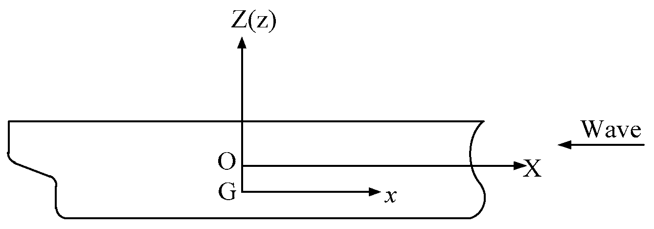
2. Mathematical Model

In order to describe the motions of a ship, two different right-handed Cartesian coordinate systems are adopted as shown in Figure 1. The first is the inertial reference frame OXYZ fixed in space, with the OX axis in mean free surface, pointing to the heading of the floating structure, and the OZ axis pointing upward. The second is the body-fixed reference frame Gxyz, with its origin coinciding with the center of gravity, G, of the floating structure. At the initial moment, the reference frame Gxyz coincides with the reference frame OXYZ.

With respect to the defined coordinate systems, the coupled heave–pitch motion of ships can be described by two linear coupled second-order ordinary differential equations of the form

$$\{\begin{array}{l}\left(M+M_{33}\right)\ddot{z}+D_{33}\dot{z}+C_{33}z+M_{35}\ddot{\theta }+D_{35}\dot{\theta }+C_{35}\theta =F_3\\ \left(I_{yy}+J_{yy}\right)\ddot{\theta }+D_{55}\dot{\theta }+C_{55}\theta +M_{53}\ddot{z}+D_{53}\dot{z}+C_{53}z=M_5\end{array}$$

(1)

where z and θ are the heave linear displacement and pitch angle, respectively; M and I_yy are the mass of inertia and pitch moment of inertia, respectively; M₃₃ and J_yy are the added mass and added moment of inertia, respectively; D_ii and C_ii, $i=3,5$ are the damping coefficients and the restoring moment coefficients, respectively; M_ij, D_ij, and C_ij, $i,j=3,5$ are the coupled hydrodynamic coefficients; F₃ and M₅ are the wave exciting force and moment, respectively.

Multiplying Equation (1) by the inverse matrix of the inertia matrix, the normalized heave–pitch motion equations are obtained

$$\{\begin{array}{l}\ddot{z}+d_{33}\dot{z}+d_{35}\dot{\theta }+c_{33}z+c_{35}\theta =f_3\\ \ddot{\theta }+d_{53}\dot{z}+d_{55}\dot{\theta }+c_{53}z+c_{55}\theta =f_5\end{array}$$

(2)

where

$$\begin{array}{l}\left(\begin{array}{cc}{d}_{33}& d_{35}\\ d_{53}& d_{55}\end{array}\right)={\left(\begin{array}{cc}M+M_{33}& M_{35}\\ M_{53}& I_{yy}+J_{yy}\end{array}\right)}^{-1}\left(\begin{array}{cc}{D}_{33}& D_{35}\\ D_{53}& D_{55}\end{array}\right)\\ \left(\begin{array}{cc}{c}_{33}& c_{35}\\ c_{53}& c_{55}\end{array}\right)={\left(\begin{array}{cc}M+M_{33}& M_{35}\\ M_{53}& I_{yy}+J_{yy}\end{array}\right)}^{-1}\left(\begin{array}{cc}{C}_{33}& C_{35}\\ C_{53}& C_{55}\end{array}\right)\\ \left(\begin{array}{l}{f}_3\\ f_5\end{array}\right)={\left(\begin{array}{cc}M+M_{33}& M_{35}\\ M_{53}& I_{yy}+J_{yy}\end{array}\right)}^{-1}\left(\begin{array}{l}{F}_3\\ M_5\end{array}\right)\end{array}$$

(3)

For the purpose of predicting the coupled heave–pitch motion of ships in waves accurately, the normalized damping coefficients, restoring force coefficients, and wave exciting forces in Equations (2) and (3) need to determine according to ship hydrodynamics in advance. However, for a ship navigating in waves, due to the action of restoring force/moment, the ship’s heave–pitch coupling motion is a periodic reciprocating motion, so the ship’s heave–pitch coupling motion equation in waves can also be expressed as

$$\{\begin{array}{l}\ddot{z}+{\omega }_3^{2}z+G_1\left(z,\theta ,\dot{z},\dot{\theta }\right)=f_3\\ \ddot{\theta }+{\omega }_5^2\theta +G_2\left(z,\theta ,\dot{z},\dot{\theta }\right)=f_5\end{array}$$

(4)

where ω₃ is the damped frequency of heave motion; ω₅ is the damped frequency of pitch motion; the unknown functions G₁ and G₂ consist of the damping terms and part of the restoring terms.

Comparing Equation (4) with Equation (2), instead of determining eight hydrodynamic parameters in Equation (2), only the two damped frequencies of heave–pitch motion and the two hydrodynamic functions need to identify by means of the nonparametric identification method.

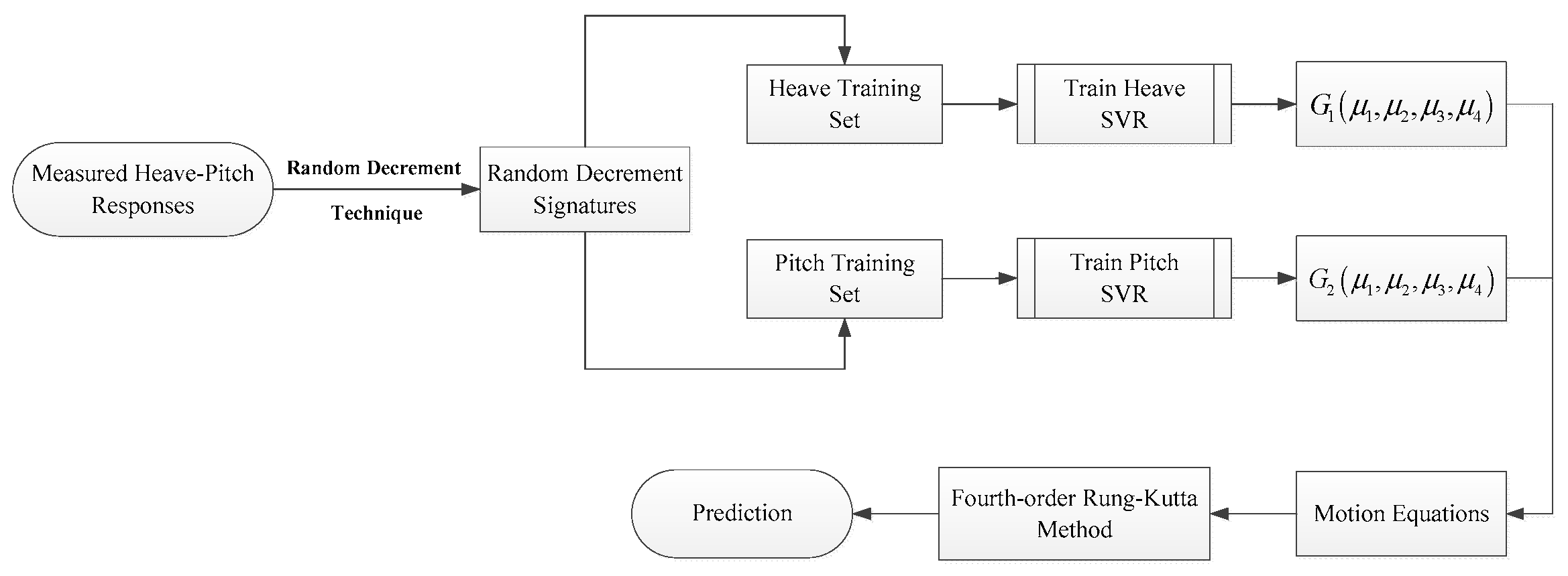
3. Identification Method

The nonparametric identification method consists of random decrement technique (RDT) and support vector regression (SVR). Therein, RDT is applied to extract random decrement signatures from ship coupled heave–pitch motion responses; and SVR is applied to identify and model unknown hydrodynamic functions.

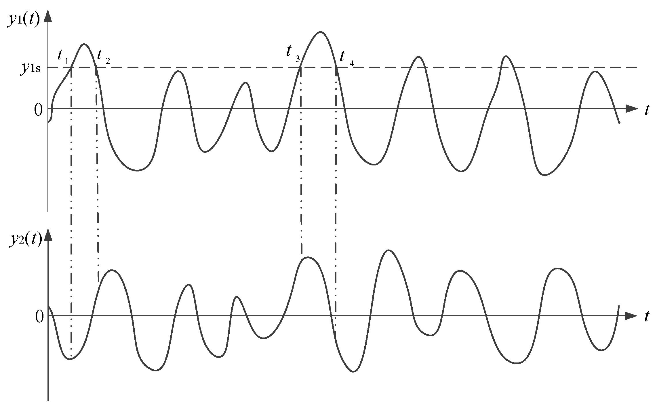
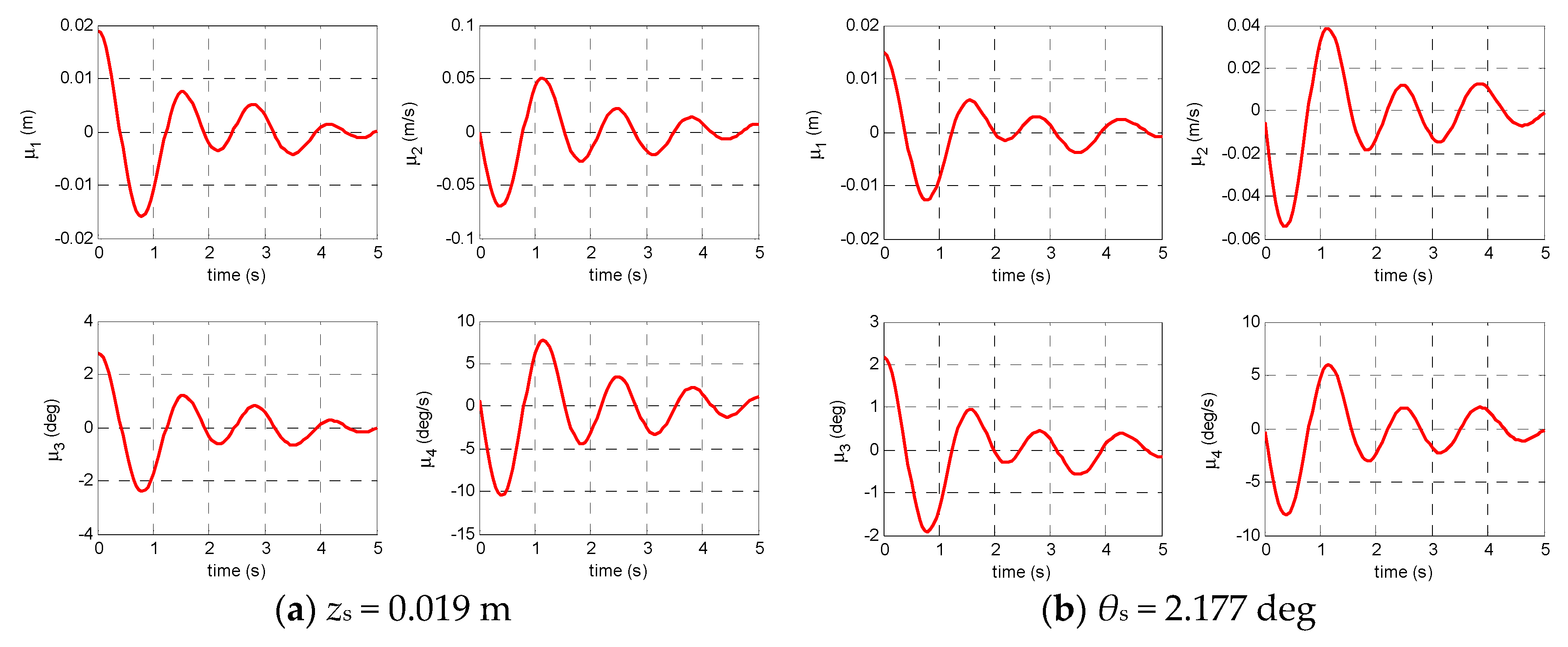
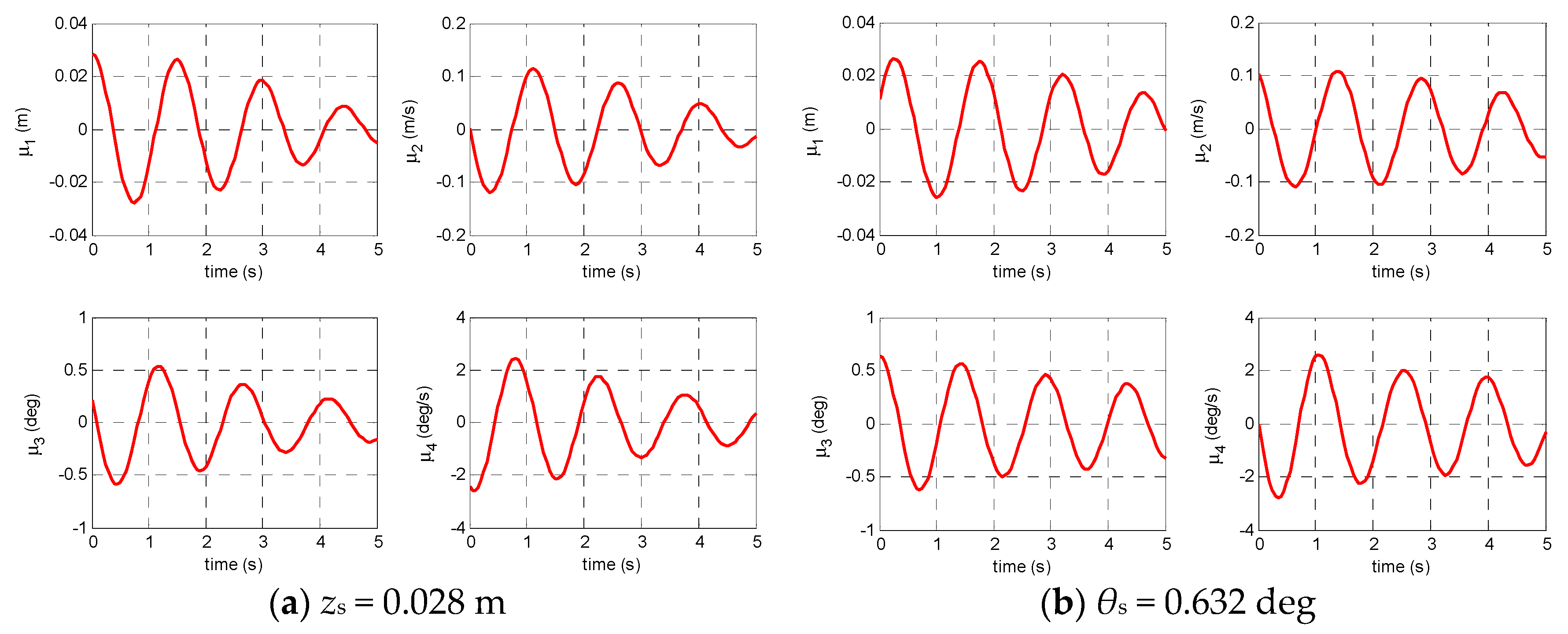
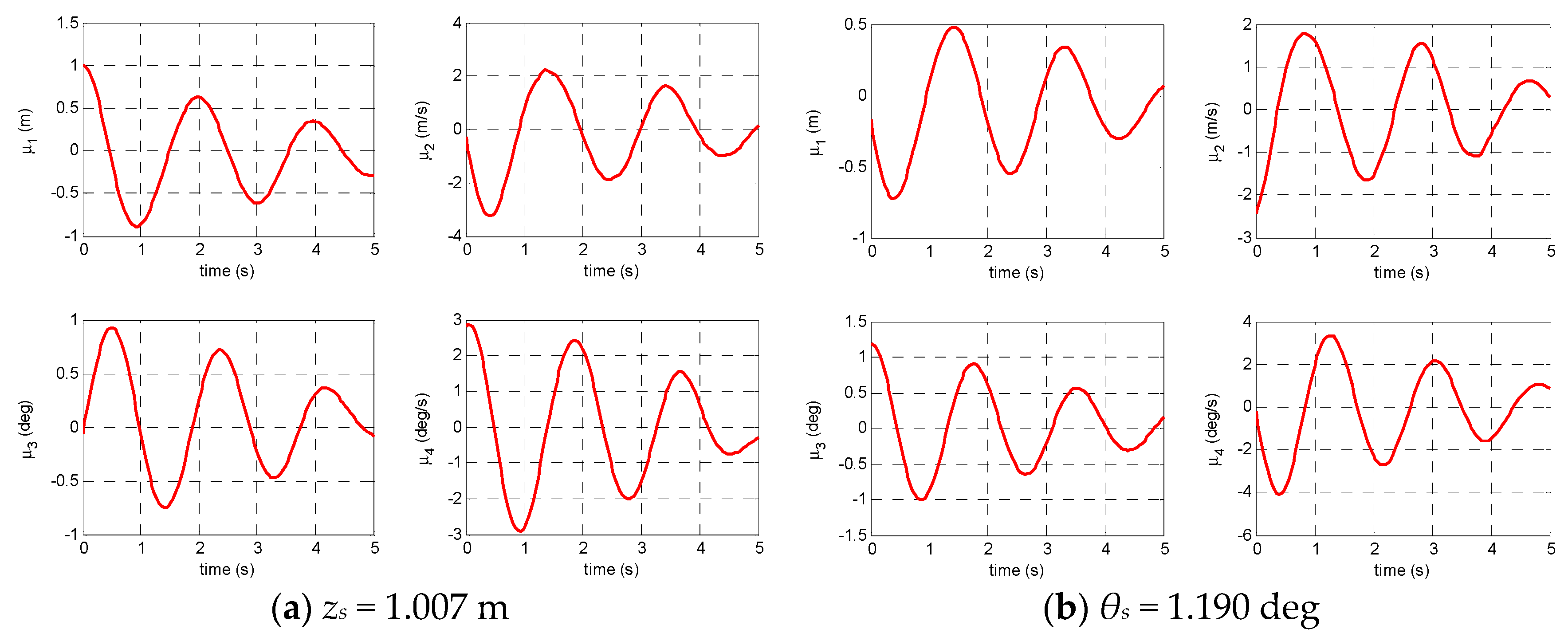
3.1. Random Decrement Technique

RDT, as an averaging technique, has been successfully applied in system identification in ship and ocean engineering [22,23]. According to the theory of RDT, the motion response of a ship in irregular waves consists of deterministic component and random component. Therein, the deterministic component is mainly determined by the initial motion state of the ship; and the random component is mainly caused by external excitation. By applying RDT on ship motion response, the random part is eliminated, leaving only the deterministic part, which is called random decrement signature.

Define the following variable substitutions

$$y_1=z, y_2=\dot{z}, y_3=\theta , y_4=\dot{\theta }, Y={\left[y_1, y_2, y_3, y_4\right]}^T$$

(5)

Substituting Equation (5) into Equation (4), it follows

$$\{\begin{array}{l}{\dot{y}}_1=y_2\\ {\dot{y}}_2=-{\omega }_3^2{y}_1-G_1\left(y_1,y_2,y_3,y_4\right)+f_3\\ {\dot{y}}_3=y_4\\ {\dot{y}}_4=-{\omega }_5^2{y}_3-G_2\left(y_1,y_2,y_3,y_4\right)+f_5\end{array}$$

(6)

Assume that the wave exciting moment satisfies the following conditions

$$\begin{array}{l}E\left[f_3\left(t\right)\right]=0, E\left[f_3\left(t_1\right)f_3\left(t_2\right)\right]={\psi }_3\delta \left(t_1-t_2\right), E\left[f_3\left(t_1\right)f_5\left(t_2\right)\right]=0\\ E\left[f_5\left(t\right)\right]=0, E\left[f_5\left(t_1\right)f_5\left(t_2\right)\right]={\psi }_5\delta \left(t_1-t_2\right), E\left[f_5\left(t_1\right)f_3\left(t_2\right)\right]=0\end{array}$$

(7)

where $E[\cdot ]$ denotes the ensemble average; ψ₃ and ψ₅ are the variances of the excitation functions; δ is the Dirac delta function.

The random process Y(t) is assumed as a Markov process, and the conditional probability density function conforms to the Fokker–Planck equation

$$\begin{array}{c}\frac{\partial P}{\partial t}=-\frac{\partial }{\partial y_1}\left(y_{2}P\right)-\frac{\partial }{\partial y_3}\left(y_{4}P\right)-\frac{\partial }{\partial y_2}\left\{\left[{\omega }_3^2{y}_1+G_1\left(y_1,y_2,y_3,y_4\right)\right]P\right\}\\ -\frac{\partial }{\partial y_4}\left\{\left[{\omega }_5^2{y}_3+G_2\left(y_1,y_2,y_3,y_4\right)\right]P\right\}+\frac{{\psi }_3}{2}\frac{{\partial }^{2}P}{\partial y_2^2}+\frac{{\psi }_5}{2}\frac{{\partial }^{2}P}{\partial y_4^2}\end{array}$$

(8)

where $P=P\left(y_1,y_2,y_3,y_4,t|y_{1,0},y_{2,0},y_{3,0},y_{4,0}\right)$ is the conditional probability density of the random process Y(t) and its initial condition is

$$\underset{t\to 0}{\lim }P\left(y_1,y_2,y_3,y_4,t|y_{1,0},y_{2,0},y_{3,0},y_{4,0}\right)=\delta (y_1-y_{1,0})\delta (y_2-y_{2,0})\delta (y_3-y_{3,0})\delta (y_4-y_{4,0})$$

(9)

where y_1,0, y_2,0, y_3,0, and y_4,0 are the initial values of the heave displacement, heave rate, pitch angle and pitch rate, respectively.

Multiply both sides of Equation (8) by the variables y₁, y₂, y₃ and y₄ respectively, and integrate the equation over the interval [−∞, ∞], and then the following equations are obtained

$$\{\begin{array}{l}{\dot{\mu }}_1={\mu }_2\\ {\dot{\mu }}_2=-{\omega }_3^2{\mu }_1-G_1\left({\mu }_1,{\mu }_2,{\mu }_3,{\mu }_4\right)\\ {\dot{\mu }}_3={\mu }_4\\ {\dot{\mu }}_4=-{\omega }_5^2{\mu }_3-G_2\left({\mu }_1,{\mu }_2,{\mu }_3,{\mu }_4\right)\end{array}$$

(10)

where μ₁, μ₂, μ₃ and μ₄ are the mean values of the heave displacement, heave rate, pitch angle and pitch rate, respectively.

Transform Equation (10) into a second-order differential equation systems

$$\{\begin{array}{l}{\ddot{\mu }}_1+{\omega }_3^2{\mu }_1+G_1\left({\mu }_1,{\mu }_2,{\mu }_3,{\mu }_4\right)=0\\ {\ddot{\mu }}_3+{\omega }_5^2{\mu }_3+G_2\left({\mu }_1,{\mu }_2,{\mu }_3,{\mu }_4\right)=0\end{array}$$

(11)

According to Equation (4), the homogenous coupled heave–pitch equation describing the free responses of heave and pitch motion can be written as

$$\{\begin{array}{l}\ddot{z}+{\omega }_3^{2}z+G_1\left(z,\theta ,\dot{z},\dot{\theta }\right)=0\\ \ddot{\theta }+{\omega }_5^2\theta +G_2\left(z,\theta ,\dot{z},\dot{\theta }\right)=0\end{array}$$

(12)

Comparing Equation (11) with Equation (12), it is obvious that the two equations have very high similarity. Therefore, the damped frequencies ω₃ and ω₅, the unknown function G₁ and G₂ in Equations (4) and (12) can be identified based on the random decrement Equation (11) and the random decrement signatures.

In this study, Figure 2 shows the procedure of obtaining the random decrement signatures. First, in order to preserve the phase shift between the coupled motions of a ship, the heave motion is selected as the reference motion and the heave displacement is correspondingly selected as the reference response. Second, the one-third significant value of the heave displacement is selected as the trigger value of random decrement signatures. Simultaneously, the time duration of the random decrement signatures is selected as 5 s. Third, the heave displacement is equally divided into N segments, and the initial value of each segment is equal to the selected trigger value. It should be noted that overlap may occur between the adjacent segments, and the initial slopes of these segments alternate between positive and negative, with half of the sections having a positive initial slope and the other half having a negative initial slope. Fourthly, each segment has the same time step and the heave displacement values at each discrete point are obtained by interpolation. Then, the values of heave displacement at each discrete point with the same sequence are superimposed and divided by the number of N segments, and the random decrement signature μ₁ of heave displacement is obtained. Finally, the random decrement signatures μ₂, μ₃, and μ₄ are obtained by using the similar procedure. The only difference is that the starting times of every segment of the other three motion responses must coincide with the starting times of the corresponding segments of the referred heave displacement.

The random decrement signatures of the coupled heave–pitch motion of a ship in irregular waves can be described as

$$\{\begin{array}{l}{\mu }_1\left(\tau \right)=\frac{1}{N}\left[{\displaystyle \sum _{i=1}^{N/2}{z}_i\left(t_i+\tau \right)}+{\displaystyle \sum _{j=1}^{N/2}{z}_j\left(t_j+\tau \right)}\right]\\ {\mu }_2\left(\tau \right)=\frac{1}{N}\left[{\displaystyle \sum _{i=1}^{N/2}{\dot{z}}_i\left(t_i+\tau \right)}+{\displaystyle \sum _{j=1}^{N/2}{\dot{z}}_j\left(t_j+\tau \right)}\right]\\ {\mu }_3\left(\tau \right)=\frac{1}{N}\left[{\displaystyle \sum _{i=1}^{N/2}{\theta }_i\left(t_i+\tau \right)}+{\displaystyle \sum _{j=1}^{N/2}{\theta }_j\left(t_j+\tau \right)}\right]\\ {\mu }_4\left(\tau \right)=\frac{1}{N}\left[{\displaystyle \sum _{i=1}^{N/2}{\dot{\theta }}_i\left(t_i+\tau \right)}+{\displaystyle \sum _{j=1}^{N/2}{\dot{\theta }}_j\left(t_j+\tau \right)}\right]\\ t=t_i, z\left(t_i\right)=z_s, \dot{z}\left(t_i\right)>0\\ t=t_j, z\left(t_j\right)=z_s, \dot{z}\left(t_j\right)<0\end{array}$$

(13)

where τ is the time length of the random decrement signature; z_s is the selected trigger value of the random decrement signature.

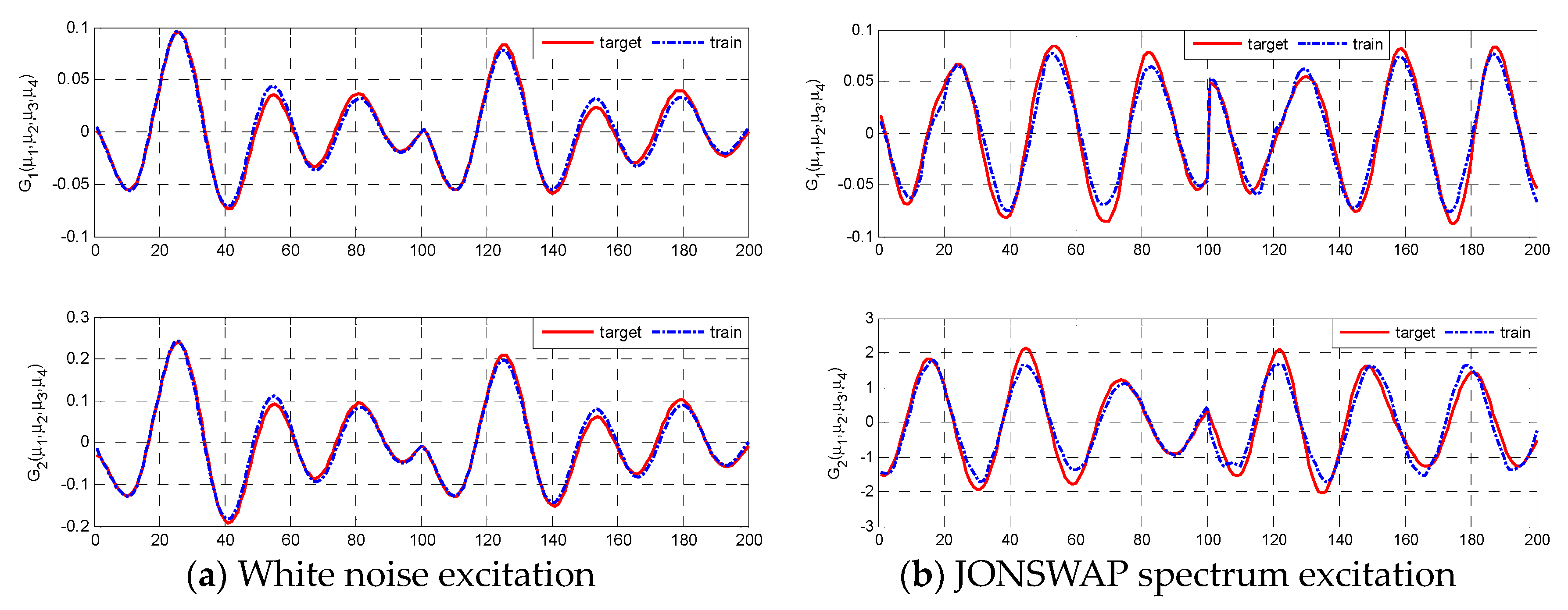
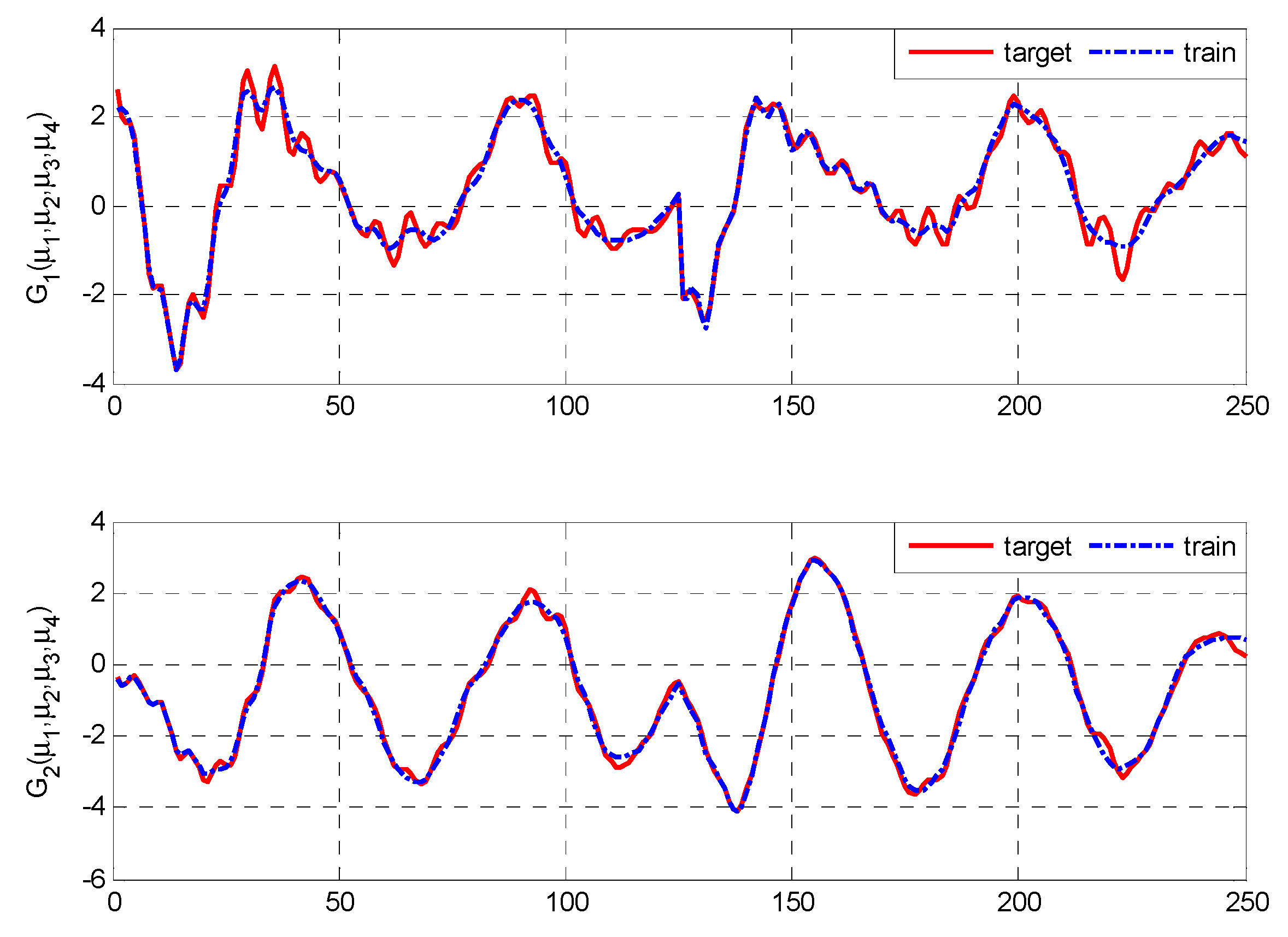
3.2. Support Vector Regression

The training set is assumed to be

$$S=\left\{\left(x_i,y_i\right),i=1,2,\cdots ,l\right\}\in {\left({\Re }^n\times \Re \right)}^l$$

(14)

where $x_i\in {\Re }^n$ is the ith n-dimension input of training set; $y_i\in \Re$ is the corresponding output of training set; l is the number of training samples; ${\Re }^n$ is the n-dimension Euclidean space and $\Re$ is the set of real numbers.

The purpose of learning based on training set is to find the feature function g(x)

$$g(x)=w^T\mathrm{\Phi }(x)+b(x\in {\Re }^n)$$

(15)

where $\mathrm{\Phi }(x)$ is a mapping function that maps the input vector x in lower dimensional space to a higher dimensional feature space by $\mathrm{X}=\mathrm{\Phi }(x)$; $w\in {\Re }^n$ is a weight matrix; $b\in \Re$ is a bias.

According to statistical learning theory, the function estimation problem of finding the characteristic function in Equation (15) by learning from the training set in Equation (14) is transformed to the following quadratic optimization problem

$$\begin{array}{l}\underset{w, {\xi }^{(\ast )}}{\min } J(w,\xi ,{\xi }^{*})=\frac{1}{2}{w}^{T}w+C{\displaystyle \sum _{i=1}^l({\xi }_i+{\xi }_i^{*})}\\ \mathrm{Subject} \mathrm{to} \left[\langle w,\mathrm{\Phi }(x_i)\rangle +b\right]-y_i\le \epsilon +{\xi }_i\\ y_i-\left[\langle w,\mathrm{\Phi }(x_i)\rangle +b\right]\le \epsilon +{\xi }_i^{*}\\ {\xi }_i, {\xi }_i^{*}\ge 0; i = 1, 2, \cdots , l\end{array}$$

(16)

where C > 0 is the penalty factor; ξ and ξ* are the slack factor vectors; $\langle \cdot ,\cdot \rangle$ denotes the inner production; ε > 0 is the insensitive zone parameter.

Define the Lagrange function

$$\begin{array}{l}{L}_f\left(w,b,\xi ,{\xi }^{*};\alpha ,{\alpha }^{*},\eta ,{\eta }^{*}\right) =\frac{1}{2}{w}^{T}w+C{\displaystyle \sum _{i=1}^l\left({\xi }_i+{\xi }_i^{*}\right)}-{\displaystyle \sum _{i=1}^l\left({\eta }_i{\xi }_i+{\eta }_i^{*}{\xi }_i^{*}\right)}\\ +{\displaystyle \sum _{i=1}^l{\alpha }_i\left(\langle w,\varphi (x_i)\rangle +b-y_i-\epsilon -{\xi }_i\right)}+{\displaystyle \sum _{i=1}^l{\alpha }_i^{*}\left(y_i-\langle w,\varphi (x_i)\rangle -b-\epsilon -{\xi }_i^{*}\right)}\end{array}$$

(17)

where ${\alpha }_i, {\alpha }_i^{\ast }, {\eta }_i, {\eta }_i^{*}\ge 0$ are introduced Lagrange multipliers.

According to the duality theorem, by introducing the Lagrange function, the original quadratic optimization problem in Equation (16) is transformed into the saddle-point problem for solving the Lagrange function

$$\underset{\alpha ,{\alpha }^{*},\eta ,{\eta }^{*}}{\max } \underset{w,b,\xi ,{\xi }^{*}}{\min } L_f\left(w,b,\xi ,{\xi }^{*};\alpha ,{\alpha }^{*},\eta ,{\eta }^{*}\right)$$

(18)

Through Equation (18), in order to obtain the optimal solution, first of all, the minimum value problem of the Lagrange function L_f with respect to parameters w, b, ξ, ξ* is solved. Moreover, the dual optimization problem of Equation (16) with respect to Lagrange multipliers is deduced based on Equation (18). It should be noted that the optimal solution of the dual optimization problem is the optimal solution of the original optimization problem in Equation (16). Finally, the optimal solution is obtained by solving the dual optimization problem with suitable numerical algorithm.

According to the conditions of the minimum value, the partial derivatives of L_f with respect to the primal variables have to vanish for optimality. It follows

$$\{\begin{array}{l}\frac{\partial L_f}{\partial w}=0\to w={\displaystyle \sum _{i=1}^l({\alpha }_i^{*}-{\alpha }_i)\mathrm{\Phi }(x_i)}\\ \frac{\partial L_f}{\partial b} =0\to {\displaystyle \sum _{i=1}^l({\alpha }_i-{\alpha }_i^{*})}=0\\ \frac{\partial L_f}{\partial {\xi }_i} =0\to {\alpha }_i+{\eta }_i=C\\ \frac{\partial L_f}{\partial {\xi }_i^{*}}=0\to {\alpha }_i^{*}+{\eta }_i^{*}=C\end{array}$$

(19)

By substituting Equation (19) into Equation (18), the dual optimization problem of the original optimization problem in Equation (16) can be obtained

$$\begin{array}{l}\underset{\alpha ,{\alpha }^{*}}{\min } W(\alpha ,{\alpha }^{*})=\frac{1}{2}{\displaystyle \sum _{i=1}^l{\displaystyle \sum _{j=1}^l({\alpha }_i^{*}-{\alpha }_i)({\alpha }_j^{*}-{\alpha }_j)K(x_i,x_j)}}+\epsilon {\displaystyle \sum _{i=1}^l({\alpha }_i^{*}+{\alpha }_i)}-{\displaystyle \sum _{i=1}^l{y}_i({\alpha }_i^{*}-{\alpha }_i)}\\ \mathrm{subject} \mathrm{to} {\displaystyle \sum _{i=1}^l({\alpha }_i-{\alpha }_i^{*})}=0, {\alpha }_i, {\alpha }_i^{*}\in \left[0, C\right]\end{array}$$

(20)

where K is the kernel function matrix and its element K(x_i, x_j) equals to the inner product of the two input vectors in the higher dimensional feature space.

Similarly, by substituting Equation (19) into Equation (15), the target feature function of SVR can be rewritten as

$$g(x)={\displaystyle \sum _{i=1}^N({\alpha }_i^{\ast }-{\alpha }_i)K(x_i,x)}+b$$

(21)

where N is the number of support vectors.

Through Equation (20), it is clear that the dual optimization problem is a convex quadratic programming problem, and therefore theoretically the local optimal solution is the global optimal solution. For the purpose of solving the dual optimization problem in Equation (20) to obtain the global optimal solution of the original optimization problem in Equation (16), any kind of optimization algorithms for solving quadratic programming problem can be used, such as inner point method, effective set algorithm, etc. In the present study, to improve the efficiency of solving the dual optimization problem, the sequential minimum optimization (SMO) algorithm [24] is selected. Compared with the traditional optimization algorithms for solving quadratic programming problem, the biggest advantage of the SMO algorithm is to train SVR analytically rather than explicitly calling a time-consuming numerical quadratic programming optimizer. The basic procedure of the SMO algorithm consists of three steps:

First, the Lagrange multipliers ${\alpha }_k, {\alpha }_k^{*}, k=1,2,\cdots ,l$ and the SVR bias b are initialized with arbitrary value, respectively;

Second, two Lagrange multipliers that violate the optimality conditions in Equation (19) is chosen by the heuristics search algorithm, and a quadratic optimization problem for the two selected variables is constructed as follows

$$\begin{array}{c}W({\lambda }_i,{\lambda }_j)={\displaystyle \sum _{k=1, k\ne i,j}^l{\lambda }_k{\lambda }_{i}K(x_k,x_i)}+{\displaystyle \sum _{k=1, k\ne i,j}^l{\lambda }_k{\lambda }_{j}K(x_k,x_j)}+\frac{1}{2}{\lambda }_i^{2}K(x_i,x_i)\\ +{\lambda }_i{\lambda }_{j}K(x_i,x_j)+\frac{1}{2}{\lambda }_j^{2}K(x_j,x_j)+\epsilon \left|{\lambda }_i\right|+\epsilon \left|{\lambda }_j\right|-y_i{\lambda }_i-y_j{\lambda }_j\end{array}$$

(22)

where ${\lambda }_k={\alpha }_k^{*}-{\alpha }_k$;

Finally, the optimal solution of the above quadratic optimization problem is solved, and the bias b and the training error of SVR are updated respectively by substituting the optimal solution into Equations (20) and (21). After that, go to the second step until all the Lagrange multipliers satisfy the optimality conditions in Equation (19). If no two Lagrange multipliers are found to violate the optimality conditions, the iterative calculation is terminated and the SVR is trained.

4. Nonparametric Identification

In this section, the proposed method consisting of RDT and SVR is applied to nonparametric identification model for ship coupled heave–pitch motion by using the random responses in irregular waves.

Firstly, the random decrement signatures of the coupled heave–pitch motion are extracted from the random responses by use of the random decrement technique. Therein, the pitch angle and the heave displacement are selected as the reference response, respectively. The significant value of the reference response, i.e., the arithmetic mean of the one-third maximum reference response, is selected as the trigger value of the random decrement signatures and the time duration is selected as 5 s. From the obtained random decrement signatures, the damped frequencies ω₃ and ω₅ can be determined.

Secondly, according to Equations (10) and (11), the discretized random decrement equation is obtained by the numerical difference.

$$\{\begin{array}{l}{G}_{1,n}\left({\mu }_{1,n},{\mu }_{2,n},{\mu }_{3,n},{\mu }_{4,n}\right)=\frac{{\mu }_{2,n}-{\mu }_{2,n+1}}{h}-{\omega }_{3,i}^2{\mu }_{1,n}\\ G_{2,n}\left({\mu }_{1,n},{\mu }_{2,n},{\mu }_{3,n},{\mu }_{4,n}\right)=\frac{{\mu }_{4,n}-{\mu }_{4,n+1}}{h}-{\omega }_{5,i}^2{\mu }_{3,n}\end{array}$$

(23)

where G_1,n denotes the value of the function G1 at the nth time step; μ_1,n is the random decrement signature of heave displacement at the nth time step; h is the time step size; ω_3,i and ω_5,i are the identified damped frequencies from the random decrement signatures.

According to Equation (23), the training samples set of SVR are constructed as

$$\begin{array}{l}\mathrm{Heave}: \mathrm{Input} =\left\{{\mu }_{1,n}; {\mu }_{2,n}; {\mu }_{3,n}; {\mu }_{4,n}\right\}\\ \mathrm{Output}=\left\{\frac{{\mu }_{2,n}-{\mu }_{2,n+1}}{h}-{\omega }_{3,i}^2{\mu }_{1,n}\right\}\\ \mathrm{Pitch}: \mathrm{Input} =\left\{{\mu }_{1,n}; {\mu }_{2,n}; {\mu }_{3,n}; {\mu }_{4,n}\right\}\\ \mathrm{Output}=\left\{\frac{{\mu }_{4,n}-{\mu }_{4,n+1}}{h}-{\omega }_{5,i}^2{\mu }_{3,n}\right\}\end{array}$$

(24)

Thirdly, the kernel function, the penalty parameter C, and the insensitive zone parameter ε need to choose for SVR in advance. In this paper, the Gauss radial basis function expressed in Equation (25) is selected as the kernel function of SVR,

$$K\left(x,x^{\prime }\right)=\exp \left(-{\Vert x-x^{\prime }\Vert }^2/2{\sigma }^2\right)$$

(25)

where σ means the width parameter of kernel function.

The penalty parameters C, the insensitive zone parameter 𝜀 and the width parameter σ are chosen by the grid search method. With respect to the constructed training samples set, the dual optimization problem in Equation (20) can be constructed and solved by the SMO algorithm.

Finally, comparing Equation (23) with the feature function of SVR in Equation (21), once the training process of SVR is finished, the unknown function G₁ and G₂ can be substituted by the trained SVR model. Substitute the identified damped frequencies and the trained SVR model into Equation (11); it is transformed into the following form

$$\{\begin{array}{l}{\ddot{\mu }}_1+{\omega }_{3,i}^2{\mu }_1+\boxed{{\mathrm{SVR}}_h({\mu }_1,{\mu }_2,{\mu }_3,{\mu }_4)}=0\\ {\ddot{\mu }}_3+{\omega }_{5,i}^2{\mu }_3+\boxed{{\mathrm{SVR}}_p({\mu }_1,{\mu }_2,{\mu }_3,{\mu }_4)}=0\end{array}$$

(26)

where $\boxed{{\mathrm{SVR}}_h({\mu }_1,{\mu }_2,{\mu }_3,{\mu }_4)}$ and $\boxed{{\mathrm{SVR}}_p({\mu }_1,{\mu }_2,{\mu }_3,{\mu }_4)}$ are the trained SVR model for heave and pitch, respectively. Integrating Equation (26) by the fourth order Rung–Kutta method, the random decrement signatures can be predicted.

Figure 3 gives the flow chart of the proposed nonparametric identification method.

To validate the applicability, accuracy and the generalization ability of the proposed identification method, case studies based on the simulated data of a ship model and the experimental data of a FPSO model are designed, respectively.

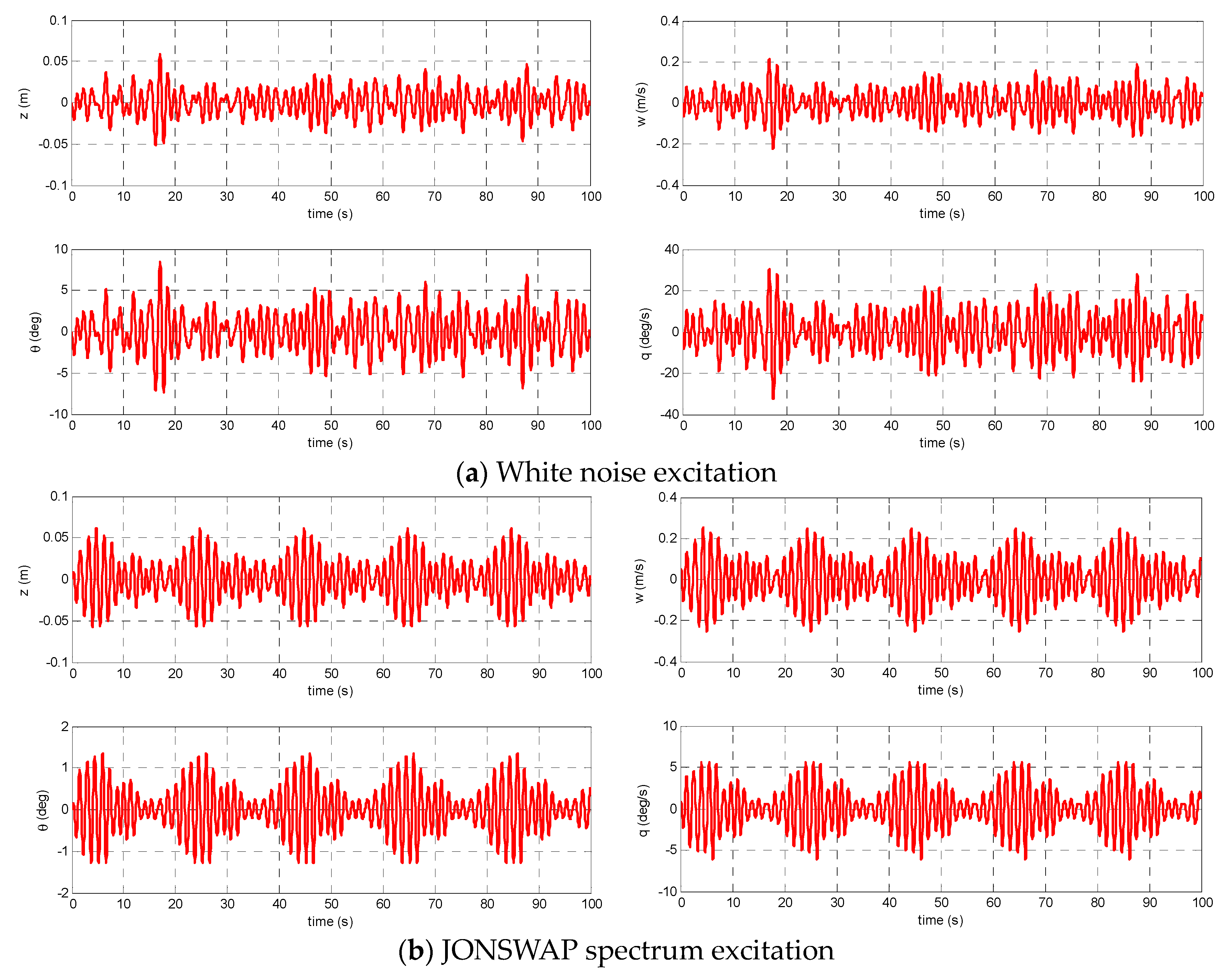
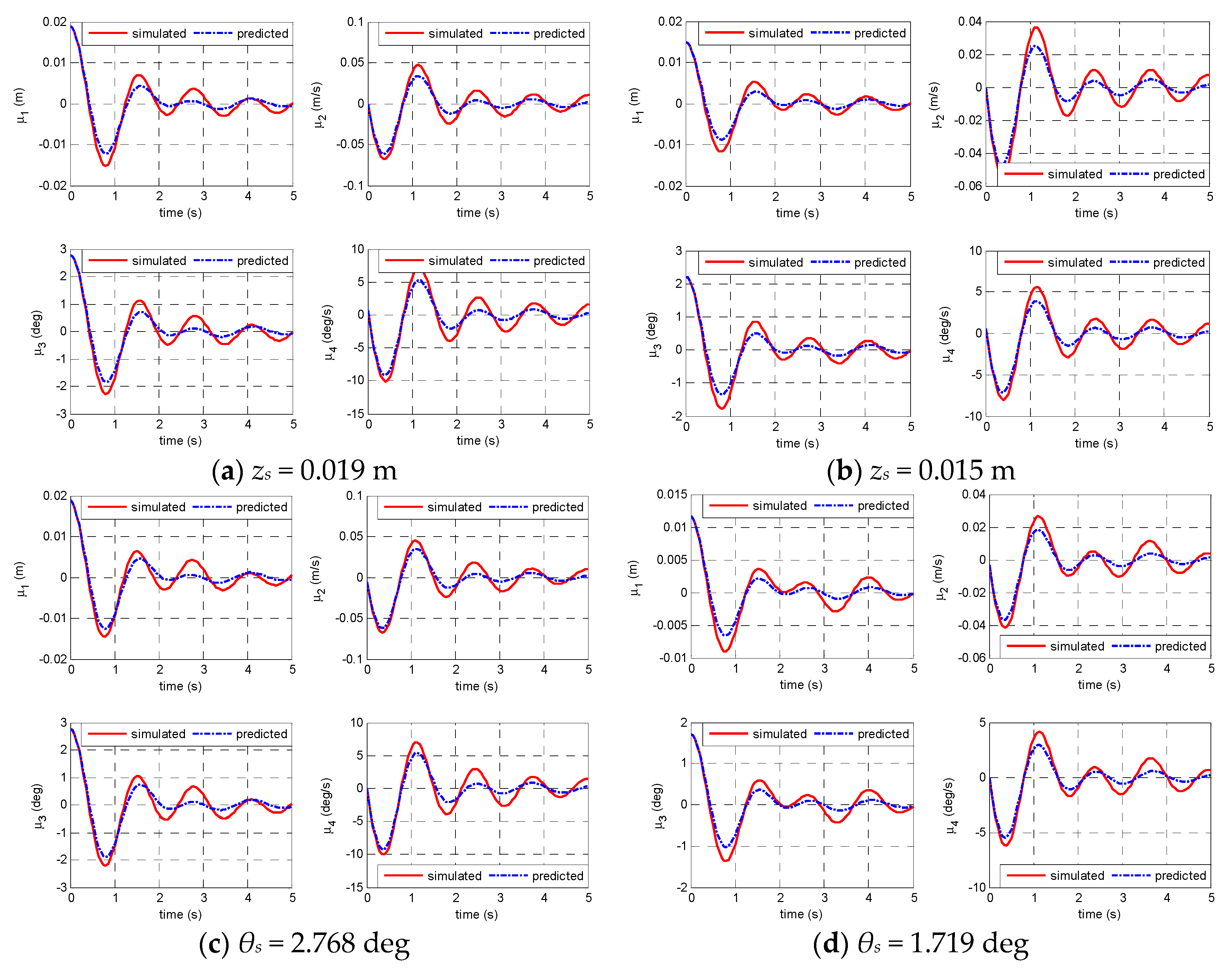
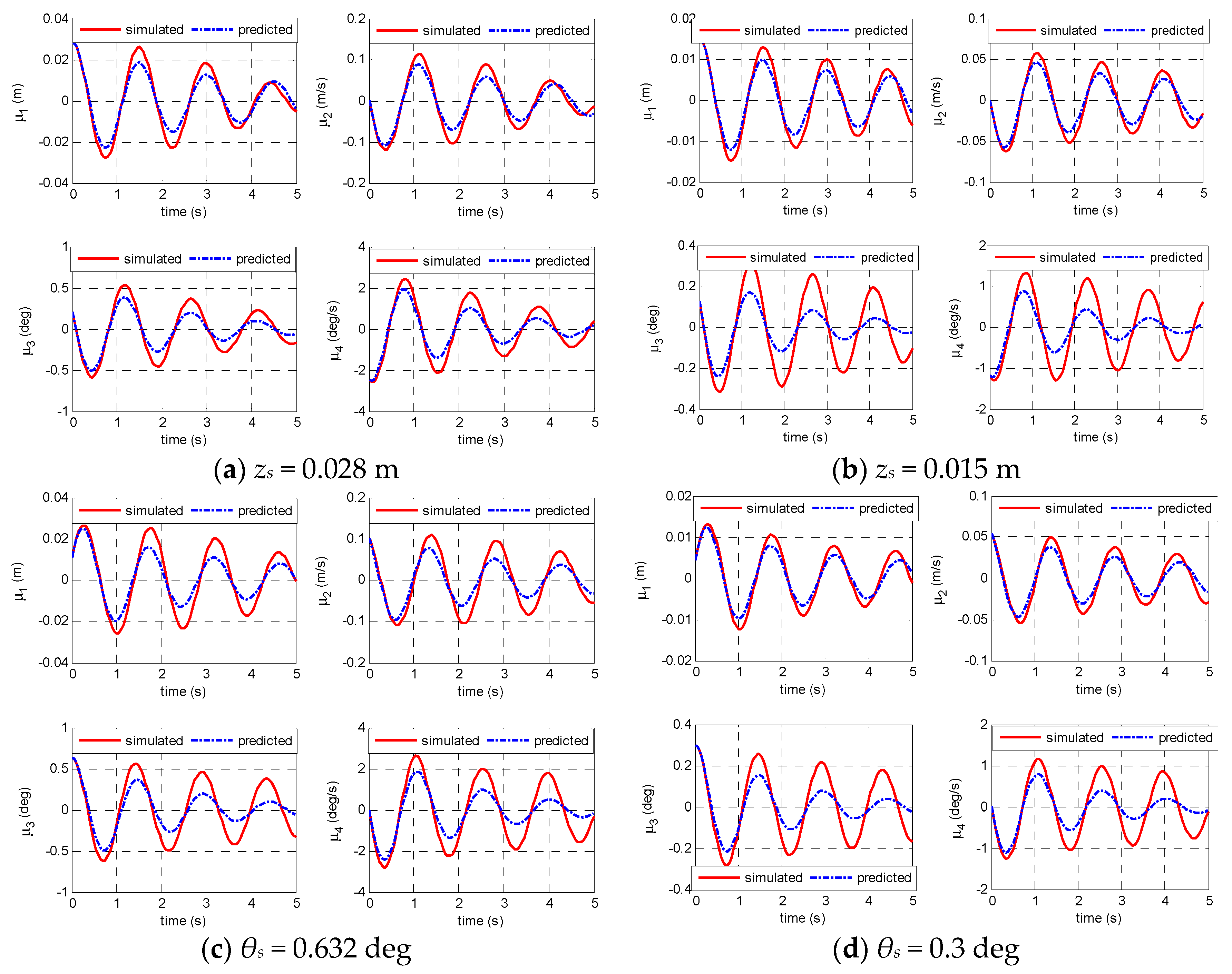
4.1. Identification Example Based on the Simulated Data

In order to test the accuracy and validity of the parametric identification procedure, the coupled heave–pitch motion of a vessel model [25] is simulated. The principal dimensions of the vessel model are given in

Table 1. Principal dimensions of the vessel model.

Item	Symbol	Unit	Value
Length between perpendiculars	Lpp	m	2.1985
Length of waterline	Lwl	m	2.3250
Breadth	B	m	0.4840
Mean draft	T	m	0.1735
Displacement volume	$\nabla$	m3	0.1190
Wetted surface area	S	m2	1.1335
Transverse metacentric radius	Rx	m	0.122
Longitudinal metacentric radius	Ry	m	2.4

, and the mathematical model for simulating the coupled heave–pitch motion of the vessel model is given in Equation (27).

$$\{\begin{array}{l}\ddot{z}+2.823\dot{z}+0.157\dot{\theta }+34.096z+0.223\theta =f_3\\ \ddot{\theta }+0.579\dot{z}+2.632\dot{\theta }+0.626z+30.785\theta =f_5\end{array}$$

(27)

For simulating the random responses, the white noise and the JONSWAP spectrum are used as the external excitation, respectively.

With respect to the white noise excitation, the normalized wave exciting force f₃ and moment f₅ are consisted of 70 sinusoidal components with constant amplitude 0.07 m/s² and 0.15 rad/s². The frequency range of the excitation is taken between 2.0 and 5.0 rad/s. The wave exciting force and moment are expressed as

$$\{\begin{array}{l}{f}_3(t)={\displaystyle \sum _{i=1}^{70}0.07\cos ({\omega }_{i}t+{\alpha }_i)}\\ f_5(t)={\displaystyle \sum _{i=1}^{70}0.15\cos ({\omega }_{i}t+{\alpha }_i)}\end{array}$$

(28)

where α_i is the phase shift between these wave exciting force components and taken as a random variable uniformly distributed between 0 and 2π.

With respect to the JONSWAP spectrum excitation, the significant height and the modal frequency of the wave spectrum are 0.05 m and 4.398 rad/s, respectively. The frequency range of the external excitation is taken between 0 and 4π rad/s. The normalized wave exciting force f₃(t) and moment f₅(t) are assumed to be consisted of 70 sinusoidal components with different amplitudes. The wave exciting force and moment are expressed as

$$\{\begin{array}{l}{f}_3(t)={\displaystyle \sum _{i=1}^{70}{f}_{3A,i}\cos ({\omega }_{i}t+{\alpha }_i)}\\ f_5(t)={\displaystyle \sum _{i=1}^{70}{f}_{5A,i}\cos ({\omega }_{i}t+{\alpha }_i)}\end{array}$$

(29)

where f_3A,i and f_5A,i are the amplitudes of the wave exciting force components, respectively.

Substituting Equations (28) and (29) into Equation (27) and taking 0.05 s as the time step size, the Equation (27) can be solved by the fixed-step fourth order Runge–Kutta method. The simulated heave and pitch coupled motion responses of the ship model under the two external excitations are obtained and shown in Figure 4. In this figure, the symbol “w” and “q” denote the heave speed and the pitch rate, respectively.

By using RDT, the random decrement signatures are extracted from the simulated data. In the present study, two kinds of random decrement signatures are obtained: one is obtained in the case that the heave displacement is selected as the reference motion; the other is obtained in the case that the pitch angle is selected as reference motion. For the white noise excitation, the trigger values of the two kinds of random decrement signatures are selected as: z_s = 0.019 m in the case of the heave displacement as the reference motion; θ_s = 2.177 deg in the case of the pitch angle as the reference motion. For the JONSWAP spectrum excitation, the trigger values are selected as: z_s = 0.028 m in the case of the heave displacement as the reference motion; θ_s = 0.632 deg in the case of the pitch angle as the reference motion. The random decrement signatures, which are extracted from the simulated heave and pitch coupled responses under the white noise excitation and the JONSWAP spectrum excitation, are shown in Figure 5 and Figure 6, respectively.

By analyzing the random decrement signatures, the damped frequencies of heave and pitch motions are identified and given in

Table 2. Identified damped frequency.

		White Noise Excitation		JONSWAP Spectrum Excitation
Frequency	Known	Identified	Error (%)	Identified	Error (%)
ω3	4.488	4.483	0.111	4.171	7.063
ω5	4.597	4.533	1.392	4.379	4.742

in comparison with the known values. From Table 2, it clearly demonstrates that the identified damped frequencies under the white noise excitation are more accurate than the identified values under the JONSWAP spectrum excitation.

According to Equation (24), the training set is constructed. The penalty parameter C, the insensitive zone parameter 𝜀, and the width parameter σ of the Gauss radial basis kernel function are selected as: C = 10⁵, 𝜀 = 0.05, σ = 0.5 for the white noise excitation; C = 1, 𝜀 = 0.05, σ = 2.5 for the JONSWAP spectrum excitation. After that, the SMO algorithm is applied to train SVR, and the training results are shown in Figure 7.

From Figure 7, it is seen that the trained SVR model describes the constructed training samples accurately. It means that the function G₁(y₁, y₂, y₃, y₄) and G₂(y₁, y₂, y₃, y₄) can be substituted by the trained SVR model. For the purpose of validating the identified results, the identified damped frequencies and the identified SVR model of the unknown function are substituted into the random decrement equation to predict the random decrement signatures. Integrating Equation (26) by the fourth order Rung–Kutta method, the random decrement signatures with different reference responses and different trigger values are predicted. The predicted random decrement signatures are shown in Figure 8 and Figure 9, respectively, in comparison with that obtained from the simulated responses by using the random decrement technique.

In Figure 8 and Figure 9, the heave displacement is selected as the reference response of the random decrement signatures in Figure 8a,b with different trigger values, and the pitch angle is selected as the reference response of the random decrement signatures in Figure 8c,d with different trigger values. From these two figures, it can be seen that the predicted random decrement signatures are generally reasonable though there are some discrepancies between the predicted results and the simulated results. The discrepancies may be ascribed to the factor of the SVR’s parameters. Although the grid search method is used, the selected penalty parameter C, the insensitive zone parameter ε and the width parameter σ may be not optimal. Actually, a universal and effective method for the selection of the optimal SVR’s parameters is still challenging.

Moreover, the identified damped frequencies and SVR models are submitted into Equation (26) to predict the coupled heave–pitch motion in irregular waves. The predicted results are compared with the simulated responses and shown in Figure 10 and Figure 11 together with the time histories of prediction errors, respectively. The prediction errors are calculated by

$$\{\begin{array}{l}{z}_{error}=\frac{z_p-z_k}{z_{rms}}\times 100\%, w_{error}=\frac{w_p-w_k}{w_{rms}}\times 100\%\\ {\theta }_{error}=\frac{{\theta }_p-{\theta }_k}{{\theta }_{rms}}\times 100\%, q_{error}=\frac{q_p-q_k}{q_{rms}}\times 100\%\end{array}$$

(30)

where the subscripts ‘p’ and ‘k’ denote the predicted and known values, respectively; the subscript ‘rms’ denotes the root-mean-square value.

From Figure 10 and Figure 11, it is seen that the coupled heave–pitch motion can be predicted using the identified damped frequencies and SVR models. Therefore, it can be concluded that the nonparametric method can be applied to identify the dynamic characteristics of the coupled heave and pitch motions of ships in irregular waves based on the simulation data.

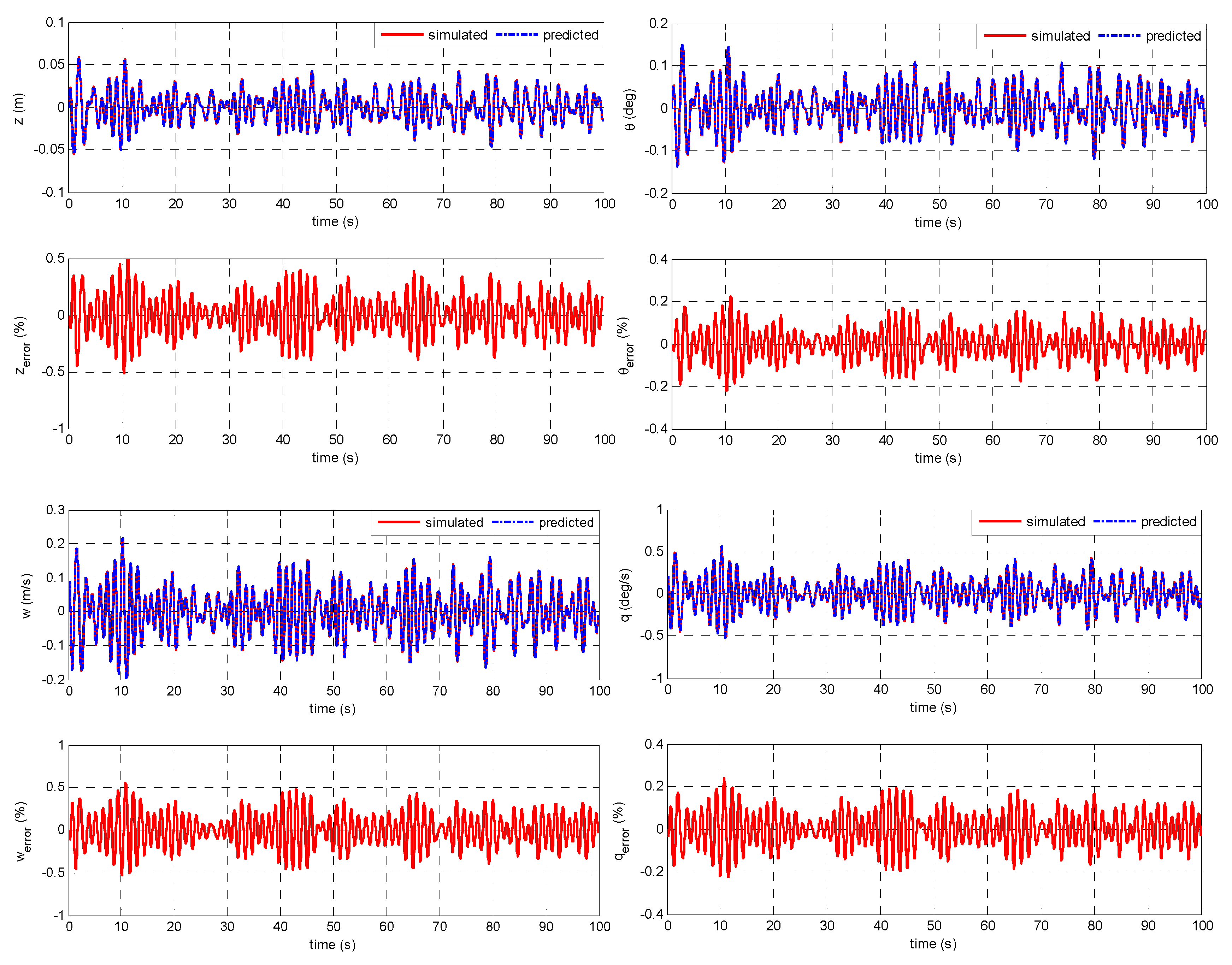
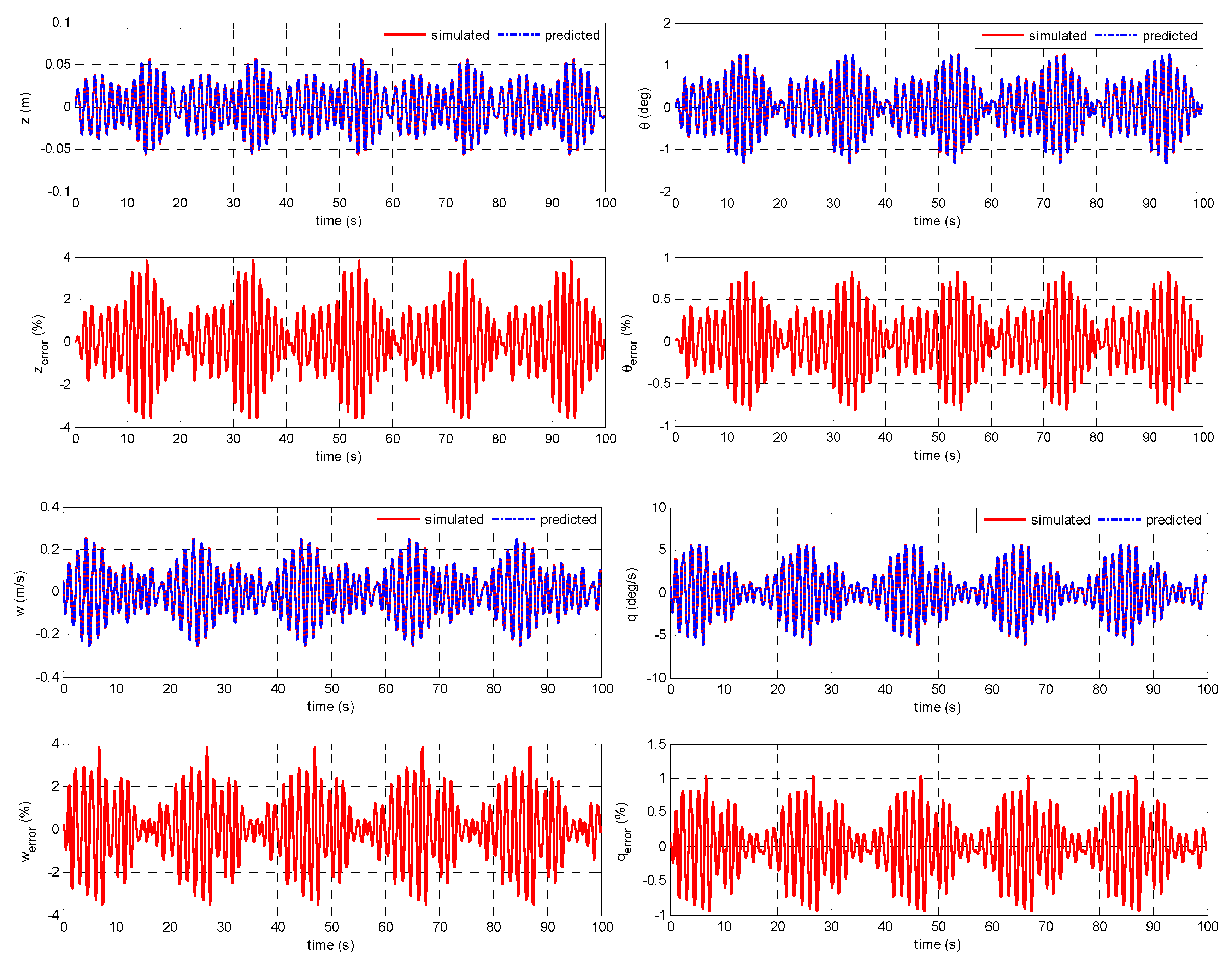
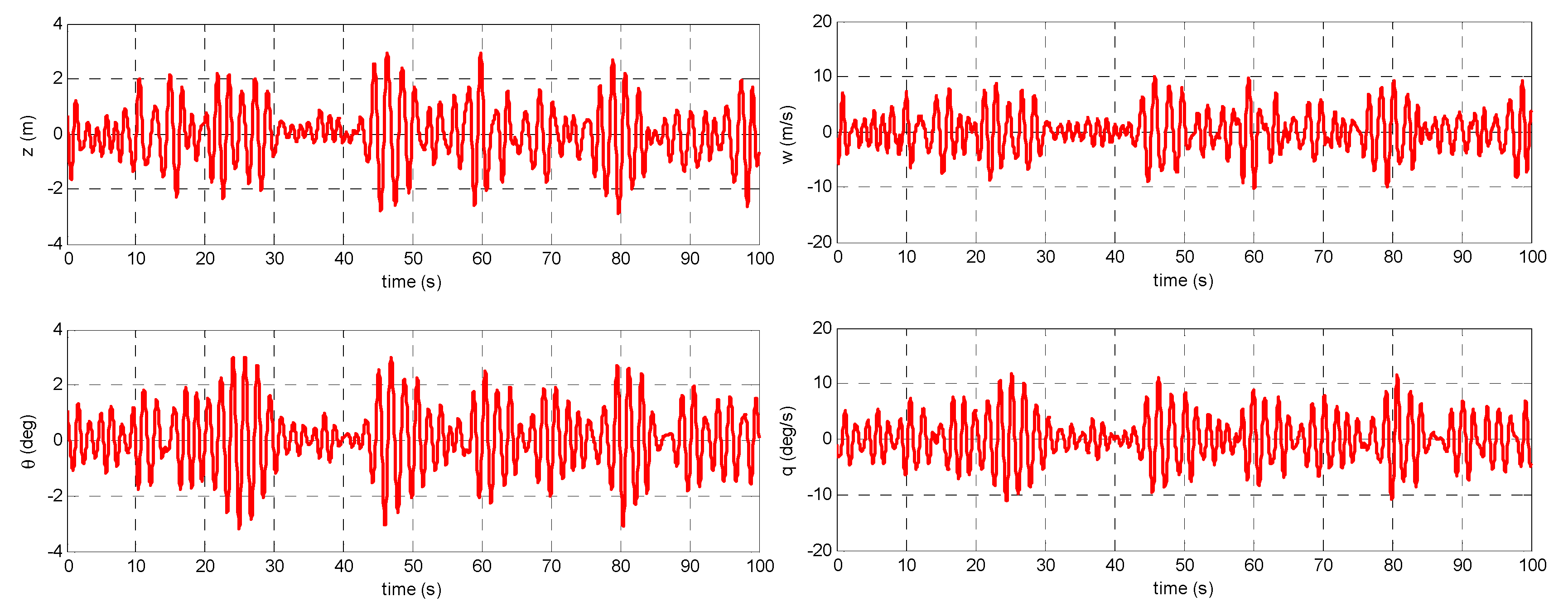
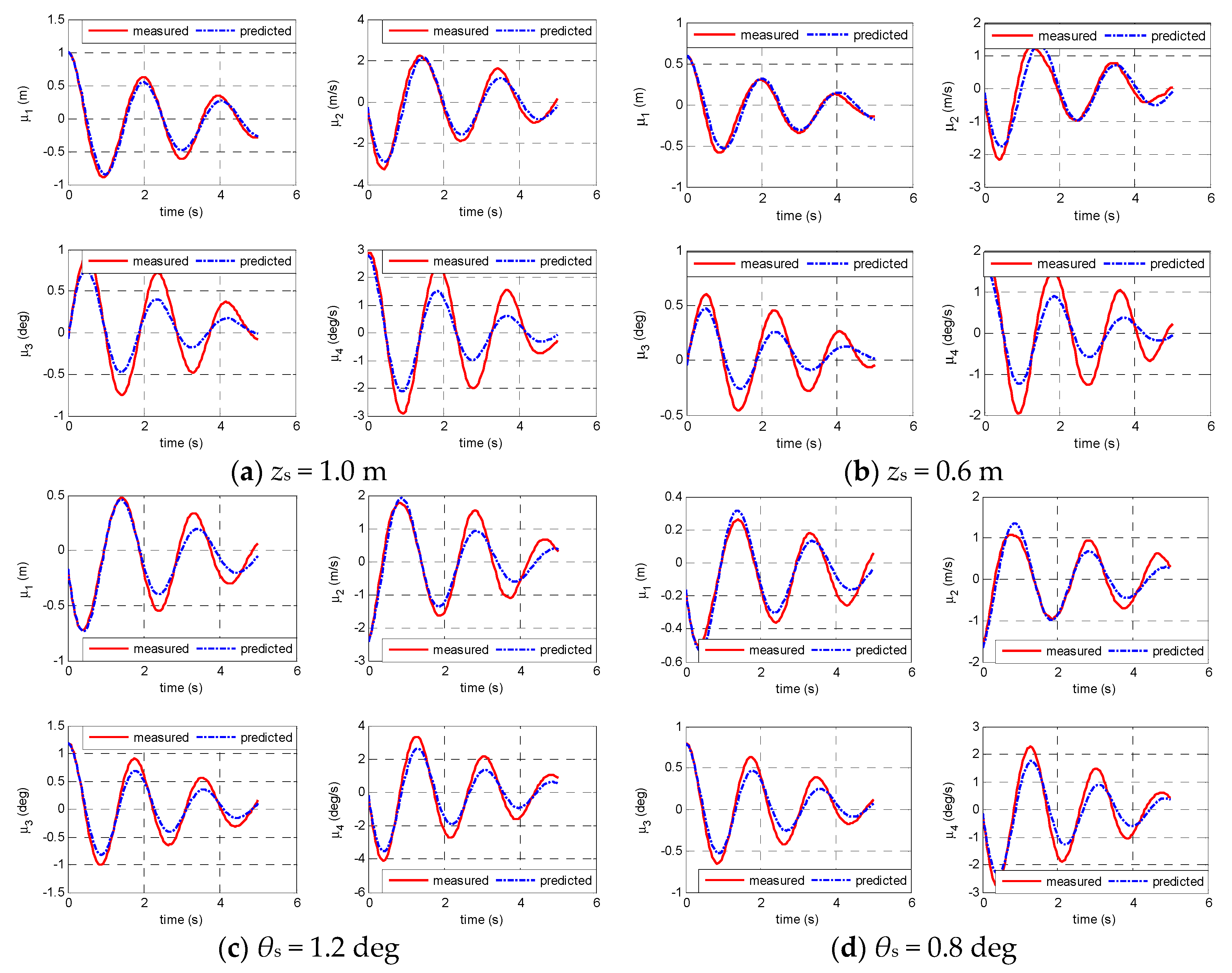
4.2. Validation/Verification Based on the Experimental Data

For the purpose of validating the applicability and generalization ability of the proposed method, it is applied to identify the coupled heave–pitch motion of a FPSO model by analyzing the measured heave and pitch coupled responses in irregular waves.

The model scale is 1:81 and the principal dimensions of the model are given in

Table 3. Principal dimensions of the FPSO model.

Item	Symbol	Unit	FPSO	Model
Length over all	Loa	m	309.31	3.82
Length between perpendiculars	Lpp	m	300.80	3.71
Breadth	B	m	54.5	0.67
Depth	D	m	25.98	0.32
Mean draft	T	m	12.5	0.15
Block coefficient	Cb	-	0.97	0.97
Radius of roll gyration	kx	m	18.4	0.23
Radius of pitch gyration	ky	m	75	0.93
Bilge keel	Lk × Bk	m	230.4 × 0.64	2.85 × 0.01

. The model is subjected to the irregular waves of the JONSWAP spectrum. The significant height of the wave spectrum is 0.1852 m, and the peak spectral period is 1.68 s. The model test condition corresponds to the 100-year survival condition at full scale, where the significant height of the wave spectrum is 15 m, and the peak spectral period is 15.1 s. The measured heave displacement and pitch angle are shown in Figure 12. Based on the measured responses, the heave speed and pitch rate are obtained by numerical differentiation and also shown in Figure 12.

By the random decrement technique, two kinds of random decrement signatures are extracted from the measured motion responses. One is obtained on a basis of the heave displacement as the reference response and z_s = 1.007 m as the trigger value; the other is obtained on a basis of the pitch angle as the reference response and θ_s = 1.190 deg as the trigger value. The obtained random decrement signatures are shown in Figure 13.

By analyzing the random decrement signatures, the damped frequencies of heave and pitch in irregular waves are identified and given in

Table 4. Identified damped frequencies of the FPSO model.

Frequency	ω3	ω5
Value	3.037	3.649

. Because of the true values of the damped frequencies are unknown, the accuracy of the identified results cannot be clearly shown by use of the comparison between the identified values and the true values in this table.

Based on the obtained random decrement signatures of the heave and pitch motion, the training set is constructed according to Equation (24), and the penalty parameter C, the insensitive zone parameter 𝜀, and the width parameter σ of the Gauss radial basis kernel function are selected as C = 100, ε = 2.5, σ = 20, respectively. Then SVR is trained by the SMO algorithm and the training results are shown in Figure 14.

From Figure 14, it is clearly seen that the SVR can describe the constructed training samples set accurately. It means that the function G₁(y₁, y₂, y₃, y₄) and G₂(y₁, y₂, y₃, y₄) can be substituted by the trained SVR model. For the purpose of validating the identified results, the identified damped frequencies and the identified SVR model of the unknown function are used to predict the random decrement signatures. Integrating Equation (26) by the fourth order Rung–Kutta method, the random decrement signatures with different reference responses and different trigger values are predicted. The predicted random decrement signatures are shown in Figure 15 in comparison with that obtained from the measured heave and pitch coupled responses by use of the random decrement technique. In Figure 15a,b, the heave displacement is used as the reference response of the random decrement signature with different trigger values, and in Figure 15c,d, the pitch angle is used as the reference response of the random decrement signature with different trigger values.

From Figure 15, it can be seen that the agreements between the predicted random decrement signatures and that from the measured responses are generally satisfactory. The discrepancies between the predicted results and the measured results may be caused by the following reasons: the first is that the SVR’s parameters are not optimal so that the SVR model cannot represent the unknown function G₁ and G₂ in the equation precisely; the second is that the random decrement signatures cannot exactly satisfy the random decrement equation.

5. Conclusions

In the present study, RDT and SVR were combined and applied to identify the nonparametric model of ship heave and pitch coupled motion in irregular waves. To determine the unknown damped and hydrodynamic functions, the random decrement signatures were extracted by RDT from the measured motion response, and then the damped frequencies were determined, and the hydrodynamic functions were identified by SVR. In order to validate the applicability, accuracy and generalization ability of the proposed method, the simulated data and experimental data were analyzed, respectively. First, the identification method was applied to analyze the simulated data of a vessel model under the white noise excitation and the JONSWAP excitation, respectively. The satisfactory agreements between the predicted responses, identified results, and the simulated responses using the known simulated model demonstrated that the identification method can be applied to the nonparametric identification of the coupled heave–pitch motion by analyzing the simulated data. Second, the identification method was applied to the experimental data of a FPSO model in irregular waves. The reasonable agreement between the predicted responses and the measured values indicated that the proposed identification method can be applied to identify heave and pitch coupled motion in irregular waves by analyzing the model test data.

From the present study, it can be concluded that the identification method can be applied to the nonparametric identification model for coupled heave–pitch motion of ships at sea by using only the motion responses, which are relatively easy to measure. However, it must be pointed that the accuracy of the identification method needs to improve by developing a universal and effective method to find the optimal parameters of SVR. This will be the subject of a future study.

References

1. Vakilabadi, K.A.; Khedmati, M.R.; Seif, M.S. Experimental study on heave and pitch motion characteristics of a wave-piercing trimaran. Trans. FAMENA 2014, 38, 13–26. [Google Scholar]
2. Mahesh, J.R.; Nallayarasu, S.; Bhattacharyya, S.K. Assessment of nonlinear heave damping model for Spar with heave plate using free decay tests. In Proceedings of the ASME 2016, 35th International Conference on Ocean, Offshore and Arctic Engineering, Busan, Republic of Korea, 19–24 June 2016. [Google Scholar]
3. Siddiqui, M.A.; Grecoab, M.; Lugni, C.; Faltinsen, O.M. Experimental studies of a damaged ship section in forced heave motion. Appl. Ocean Res. 2019, 88, 254–274. [Google Scholar] [CrossRef]
4. Coslovich, F.; Kjellberg, M.; Östberg, M.; Janson, C.E. Added resistance, heave and pitch for the KVLCC2 tanker using a fully nonlinear unsteady potential flow boundary element method. Ocean Eng. 2021, 229, 108935. [Google Scholar] [CrossRef]
5. Simonsen, C.D.; Otzen, J.F.; Joncquez, S.; Stern, F. EFD and CFD for KCS heaving and pitching in regular head waves. J. Mar. Sci. Technol. 2013, 18, 435–459. [Google Scholar] [CrossRef]
6. Kim, B.S.; Park, D.M.; Kim, Y. Study on nonlinear heave and pitch motions of conventional and tumblehome hulls in head seas. Ocean Eng. 2022, 247, 110671. [Google Scholar] [CrossRef]
7. Sathyaseelan, D.; Hariharan, G.; Kannan, K. Parameter identification for nonlinear damping coefficient from large-amplitude ship roll motion using wavelets. Beni Suef Univ. J. Basic Appl. Sci. 2017, 6, 138–144. [Google Scholar] [CrossRef]
8. Dai, Y.; Cheng, R.; Yao, X.; Liu, L. Hydrodynamic coefficients identification of pitch and heave using multi-objective evolutionary algorithm. Ocean Eng. 2019, 171, 33–48. [Google Scholar] [CrossRef]
9. Xue, Y.F.; Liu, Y.J.; Ji, C.; Xue, G. Hydrodynamic parameter identification for ship manoeuvring mathematical models using a Bayesian approach. Ocean Eng. 2020, 195, 106612. [Google Scholar] [CrossRef]
10. Wang, S.S.; Wang, L.J.; Im, N.; Zhang, W.D.; Li, X.J. Real-time parameter identification of ship maneuvering response model based on nonlinear Gaussian Filter. Ocean Eng. 2022, 247, 110471. [Google Scholar] [CrossRef]
11. Zhao, Y.H.; Wu, J.B.; Zeng, C.H.; Huang, Y.X. Identification of hydrodynamic coefficients of a ship manoeuvring model based on PRBS input. Ocean Eng. 2022, 246, 110640. [Google Scholar] [CrossRef]
12. Jiang, Y.; Hou, X.R.; Wang, X.G.; Wang, Z.H.; Yang, Z.L.; Zou, Z.J. Identification modeling and prediction of ship maneuvering motion based on LSTM deep neural network. J. Mar. Sci. Technol. 2022, 27, 125–137. [Google Scholar] [CrossRef]
13. Hao, L.Z.; Han, Y.; Shi, C.; Pan, Z.Y. Recurrent neural networks for nonparametric modeling of ship maneuvering motion. Int. J. Nav. Archit. Ocean Eng. 2022, 14, 100436. [Google Scholar] [CrossRef]
14. Xue, Y.F.; Chen, G.; Li, Z.T.; Xue, G.; Wang, W.; Liu, Y.J. Online identification of a ship maneuvering model using a fast noisy input Gaussian process. Ocean Eng. 2022, 250, 110704. [Google Scholar] [CrossRef]
15. Hou, X.R.; Zou, Z.J. SVR-based identification of nonlinear roll motion equation for FPSOs in regular waves. Ocean Eng. 2015, 109, 531–538. [Google Scholar] [CrossRef]
16. Hou, X.R.; Zou, Z.J. Parameter identification of nonlinear roll motion equation for floating structures in irregular waves. Appl. Ocean Res. 2016, 55, 66–75. [Google Scholar] [CrossRef]
17. Hou, X.R.; Zou, Z.J.; Xu, F. SVR-based parameter identification of coupled heave-pitch motion equations in regular waves. In Proceedings of the Twenty-Sixth International Ocean and Polar Engineering Conference, Rhodes, Greece, 26 June–2 July 2016; pp. 580–585. [Google Scholar]
18. Wang, Z.H.; Zou, Z.J.; Guedes Soares, C. Identification of ship manoeuvring motion based on nu-support vector machine. Ocean Eng. 2019, 183, 270–281. [Google Scholar] [CrossRef]
19. Meng, Y.; Zhang, X.F.; Zhu, J.X. Parameter identification of ship motion mathematical model based on full-scale trial data. Int. J. Nav. Archit. Ocean Eng. 2022, 14, 100437. [Google Scholar] [CrossRef]
20. Hou, X.R.; Zou, Z.J.; Liu, C. Nonparametric identification of nonlinear ship roll motion by using the motion response in irregular waves. Appl. Ocean Res. 2018, 73, 88–99. [Google Scholar] [CrossRef]
21. Xu, H.T.; Guedes Soares, C. Manoeuvring modelling of a containership in shallow water based on optimal truncated nonlinear kernel-based least square support vector machine and quantum-inspired evolutionary algorithm. Ocean Eng. 2020, 195, 106676. [Google Scholar] [CrossRef]
22. Elshafey, A.A.; Haddara, M.R.; Marzouk, H. Identification of the excitation and reaction forces on offshore platforms using the random decrement technique. Ocean Eng. 2009, 36, 521–528. [Google Scholar] [CrossRef]
23. Kim, Y.; Park, S.G. Wet damping estimation of the scaled segmented hull model using the random decrement technique. Ocean Eng. 2014, 75, 71–80. [Google Scholar] [CrossRef]
24. Takahashi, N.; Guo, J.; Nishi, T. Global convergence of SMO algorithm for support vector regression. IEEE Trans. Neural Netw. 2008, 19, 971–982. [Google Scholar] [CrossRef] [PubMed]
25. Xu, J.S. Identification of Ship Coupled Heave and Pitch Motions Using Neural Networks. Master’s Thesis, Memorial University of Newfoundland, Norris Point, NL, Canada, 1997. [Google Scholar]
Figure 1. Coordinate systems.
Jmse 11 00676 g001
Figure 2. Illustration of two random decrement signatures.
Jmse 11 00676 g002
Figure 3. Flow chart of nonparametric identification.
Jmse 11 00676 g003
Figure 4. Simulated heave and pitch coupled responses.
Jmse 11 00676 g004
Figure 5. Random decrement signatures from simulated data, white noise excitation.
Jmse 11 00676 g005
Figure 6. Random decrement signatures from simulated data, JONSWAP spectrum excitation.
Jmse 11 00676 g006
Figure 7. Training results of SVR for the simulated data.
Jmse 11 00676 g007
Figure 8. Predicted random decrement signatures, white noise excitation.
Jmse 11 00676 g008
Figure 9. Predicted random decrement signatures, JONSWAP spectrum excitation.
Jmse 11 00676 g009
Figure 10. Comparisons between the predicted and simulated responses, white noise excitation.
Jmse 11 00676 g010
Figure 11. Comparisons between the predicted and simulated responses, JONSWAP spectrum excitation.
Jmse 11 00676 g011
Figure 12. Measured heave and pitch responses of the FPSO model.
Jmse 11 00676 g012
Figure 13. Random decrement signatures from the measured responses.
Jmse 11 00676 g013
Figure 14. Training results of SVR based on the experimental data.
Jmse 11 00676 g014
Figure 15. Comparisons between the predicted values and the measured values of the FPSO model.
Jmse 11 00676 g015