Study on the Effect of Air Injection Location on the Drag Reduction in SWATH with Air Lubrication

Abstract

In this paper, the air lubrication method is applied to high-speed SWATH (small waterplane area twin hull) to reduce the resistance. The influence of air injection locations on drag reduction is investigated. The computed results are compared with experimental results, and the grid independence test is performed. Then, the numerical method is used to simulate the resistance of SWATH in calm water with airflow. The hull is divided into different areas, and the influence of the air injection location on the drag reduction in different areas of the hull is studied through different air injection locations and airflow rates. It could be seen that the air injection location on the underwater body is more conducive to the drag reduction in SWATH than the air injection location on the strut. Besides, the air injection location near the bow of the underwater body could cause a better drag reduction effect of SWATH. There are obvious differences in the drag reduction effect of different areas of the underwater body.

1. Introduction

The SWATH (small waterplane area twin hull) has been successfully used for passenger ships, cruise ships, and research vessels [1,2,3]. The basic structure of the SWATH is two torpedo-like underwater bodies and two or more struts, which have excellent seakeeping performance. As a downside to the ideal seakeeping behaviors, generally, conventional SWATH vessels do not have high performance in terms of calm water resistance [3]. Many scholars have studied the method of reducing resistance by optimizing the SWATH shape. Brizzolara [4] obtained an optimal SWATH with a non-conventional underwater hull form by developing a viscous-inviscid CFD method in the optimization. Based on Brizzolara’s study, Qian [5] focused on optimizing inclined struts of the SWATH by hydrodynamic analysis. The numerical simulation result of SWATH with inclined struts was compared manually with vertical struts SWATH. Vernengo [3] used the multi-objective optimization method to optimize the shape of SWATH at different speeds, and the optimal result was obtained. Lin [6] set up an automatic design optimization procedure for SWATH, and a resistance reduction in 28.9% was achieved.

Nowadays, the air lubrication method has been used by more and more scholars to reduce resistance [7,8,9,10,11,12,13]. The air lubrication method is to inject air into the boundary layer through slots, porous materials, or perforated plates, and the air is mainly held in the boundary layer in the form of isolated bubbles or a continuous layer to reduce the density of the air-water mixture and to modify turbulent momentum transport [14].

The early research on the air lubrication method was mainly carried out using a flat plate. Elbing [14] uses a flat plate to investigate two distinct air lubrication methods: bubble drag reduction (BDR) and air layer drag reduction (ALDR) by experiments. In a complete view, Murai et al. [15] and Murai [16] studied the effect of bubble size and incoming flow velocity on drag reduction. Murai [15,16] reviewed the previous research and summarized the two research directions of tiny high-speed bubbles and large low-speed bubbles. Slyozkin [17] used experimental methods to change the incoming flow speed and airflow rate of a flat plate to study the propagation process of air in the bottom cavity of the plate. Amromin [18] examined the influencing factors of the stable air layer boundary with a flat plate as the object.

The air layer could be produced by injecting air from a continuous slot [19] or one or more injection holes [20]. Elbing [19] used the slots to inject airflow into the bottom of a flat plate, conducted experimental research on changing the airflow rate on a flat plate, and reported the effect of airflow rate on building the air layer to reduce the resistance and provided the critical airflow rate to construct the air layer in various conditions. Mäkiharju [20] used injection holes to inject airflow to study the influence of the injection holes’ layout on the air layer coverage and obtain a cm-level air layer.

Many studies have applied the air lubrication method to planing ships and large flat-bottom ships. Matveev [9] compared the test and numerical simulation results of a planing ship. Butterworth [8] conducted a ship model test on a container ship model with an air cavity, the test results showed that the total resistance was reduced by 4–16%, and the air layer generated by the air injecting could be kept at the bottom of the air cavity area. Pearce [21] conducted similar experiments to study the effect of varying ventilation on the Reynolds number and air layer thickness, which provided a reference for selecting the longitudinal location of the air cavity. Cucinotta [22] studied the influence of different bottom air cavity designs of planing boats on the distribution of the air layer by experimental methods, including single-step air cavities, double-step air cavities, and single-step air cavities with isolation fences. Cucinotta [10] studied the streamline and air layer distribution of a planing air tanker and observed the wet surface area and gas coverage area to explore the relationship between airflow rate, ship speed, and air distribution. Wu Hao [11,12,13] used a combination of experiment and numerical simulation to study bulk carriers’ resistance and air layer distribution with a bottom air cavity and studied the effects of different lateral and trim conditions on the air layer distribution and drag reduction. Jang [7] researched the drag reduction in the air layer under a flat plate, observed the formation of the air layer, and measured the change of local friction resistance under different airflow rates. At the same time, the method was applied to a 66K DWT bulk carrier for towing and self-propelled tests. The model resistance is converted into the corresponding full-scale ship resistance by keeping the same level reduction ratio of the frictional resistance between the model scale and the full scale, and the net energy saving was about 5–6%.

In previous research, the bottom is usually covered by the air layer or air bubbles when studying the air lubrication method. Most of the side hulls of SWATH are underwater, and the large wet surface area is one of the main problems of the SWATH form, which is the reason why the air bubbles and air layer is applicable for SWATH and deserve more research. Until now, the research on the application of the air lubrication method on SWATH is limited. Thus, it is necessary to study the effect of the airflow on the resistance and the drag reduction in SWATH.

In this paper, numerical simulations for the resistance of SWATH with air injection at high speed are carried out. The resistance is compared with the experiment results, and the grid independence test has also been taken. The SWATH moves in calm water and is fixed in an upright sailing attitude. The injection location and the airflow rate are changed to study drag reduction. The hull is divided into several areas, and every area’s resistance and drag reduction are analyzed.

2. Numerical Approaches

2.1. Numerical Model

In this study, the resistance of the ship model was simulated by the URANS codes of a commercial software. The governing equations are the RANS equations and continuity equations for the mean velocity of the unsteady three-dimensional incompressible flow. The averaged continuity and momentum equations in the tensor form in the Cartesian coordinate system are given as follows:

$$\frac{\partial \left(\mathsf{\rho }\overline{{\mathrm{u}}_{\mathrm{i}}}\right)}{\partial {\mathrm{x}}_{\mathrm{i}}}=0$$

(1)

$$\frac{\partial \left(\mathsf{\rho }\overline{{\mathrm{u}}_{\mathrm{i}}}\right)}{\partial \mathrm{t}}+\frac{\partial }{\partial {\mathrm{x}}_{\mathrm{j}}}\left(\mathsf{\rho }\overline{{\mathrm{u}}_{\mathrm{i}}{\mathrm{u}}_{\mathrm{j}}}+\mathsf{\rho }\overline{{\mathrm{u}}_{\mathrm{i}}^{’}{\mathrm{u}}_{\mathrm{j}}^{’}}\right)=-\frac{\partial \overline{\mathrm{p}}}{\partial {\mathrm{x}}_{\mathrm{i}}}+\frac{\partial \overline{{\mathsf{\tau }}_{\mathrm{ij}}}}{\partial {\mathrm{x}}_{\mathrm{j}}}$$

(2)

where $\overline{{\mathrm{u}}_{\mathrm{i}}}$ is the relative averaged velocity vector of flow between the fluid and the control volume, $\overline{{\mathrm{u}}_{\mathrm{i}}^{’}{\mathrm{u}}_{\mathrm{j}}^{’}}$ is the Reynolds stress and $\overline{\mathrm{p}}$ is the mean pressure, $\overline{{\mathsf{\tau }}_{\mathrm{ij}}}$ is the mean shear stress tensor.

The Finite Volume Method (FVM) was applied to the spatial discretization. The Volume of Fluid (VOF) method was used to model the free surface. The convection scheme used for the VOF method is the HRIC (High-Resolution Interface Capturing). It relies on the fact that the two types of fluid, air and liquid, do not interpenetrate with each other in each control cell. Thus, as long as the volume fraction of different components in the local cell is known, the parameter values of the flow field in the cell can be obtained. The VOF method can only obtain the interface between water and injected air by interpolation. However, the VOF method is still widely applied in the corresponding research as follows [10,11]. A second-order convection scheme is used throughout all the simulations to capture the interface between the phases accurately. The flow equations were solved in a segregated manner by using a predictor-corrector approach. Convection and diffusion terms in the RANS equations were discretized by a second-order upwind scheme and a central difference scheme. The semi-implicit method for the pressure-lined equations (SIMPLE) algorithm is used to resolve the pressure velocity coupling. The turbulence model used in all numerical cases is the k-omega SST model, widely used in multi-hull ships and successive air injection [10]. The k-omega SST model uses the standard k-omega model for the near-field flow near the surface and uses the k-omega model with a high Reynolds number in the far-field flow. A mixing function is used to transition the flow in the near and far fields.

2.2. Computational Domain and Mesh

The size of the computational domain has a significant influence on the grid quality and the cost of the solution. The too-large domain will increase the computational time and cost. On the other hand, the too-small domain will adversely decrease the accuracy of numerical simulation. The computational domain and the boundary conditions for the SWATH model are shown in Figure 1a. Based on the two-phase flow theory, the boundary conditions are set as follows. The distance is 0.8 times the overall length from the model’s fore to the Inlet, and the distance is 3.5 times the overall length from the model’s aft to the Outlet. The Inlet, Side, Top, and Bottom are all velocity inlet boundary conditions with a field function for the velocity and the volume fraction. The Outlet is a pressure outlet defined by a field function dependent on the free surface location. The surface of the injection gaps is treated separately from the rest of the hull. It is a Wall when there is no injection of the air and a Flow-Rate inlet when there is the injection of the air. The mesh around the underwater bodies is refined to obtain the characteristics of the air layer. In addition, the mesh has been refined for the Kelvin wake solution near the free surface. The STAR CCM+ software allows for a choice of different methods for the treatment of the boundary layer. A High Wall ${\mathrm{y}}^{+}$ treatment is used, which is calculated as follows [23]:

$${\mathrm{y}}^{+}=0.172\left(\mathrm{y}/\mathrm{L}\right){\mathrm{Re}}^{0.9}$$

(3)

The approach allows solving the boundary layer with the use of the wall functions. The distance $\mathrm{y}$ of the first point from the wall is the first near-wall prism layer thickness of the mesh. The number of prism layers is chosen to be 5, and the thickness ratio is 1.2. The first near-wall thickness could be calculated as 0.00044 m by ${\mathrm{y}}^{+}=100$. The simulation mesh is shown in Figure 1b. Mesh generation is performed by using the automatic meshing facility in STAR CCM+ software.

3. Validation and Verification

3.1. SWATH Model

The model of SWATH used for the numerical simulation and model test is shown in Figure 2. The primary dimension characteristics of the one-side hull of the SWATH are as follows: ${\mathrm{L}}_{\mathrm{OA}}=2.5 \mathrm{m}$, ${\mathrm{L}}_{\mathrm{W}}=1.1 \mathrm{m}$ ${\mathrm{r}}_{\mathrm{M}}=0.06 \mathrm{m}$, $\mathrm{B}=1.2 \mathrm{m}$, ${\mathrm{B}}_{\mathrm{M}}=1.32 \mathrm{m}$, $\mathrm{d}=0.2 \mathrm{m}$, $\mathsf{\beta }=$60°, $\Delta =$16.8 kg, where ${\mathrm{L}}_{\mathrm{OA}}$ is the overall length, ${\mathrm{L}}_{\mathrm{W}}$ is the waterline length, $\mathrm{B}$ is the distance between side hulls, ${\mathrm{B}}_{\mathrm{M}}$ is the projected maximum beam, $\mathrm{d}$ is the draft, $\mathsf{\beta }$ is the inclined angle of struts, $\Delta$ is the displacement.

The airflow is injected through the line gaps. The air injection locations are shown in Figure 3. The line gaps in the front underwater body of SWATH are cone-shaped, and the injection location L1 is arranged in the bow. The middle part is cylindrical, with three injection locations, L2, L3, and L4, in a ring shape. The struts are trapezoidal and have an inclination angle of 60°. Two injection locations, L5 and L6, are arranged inside and outside the strut. The location L1 is composed of three-line gaps, and the total length of a side hull is 0.219 m; the locations L2, L3, and L4 are composed of circular line gaps, and the lengths are 0.321 m, 0.301 m, and 0.356 m, respectively. The purple line in Figure 3 is the line gaps of injection locations L5 and L6 on the inner side of the strut, and there are other line gaps of the half-height on the outer side of the strut, too. In the model test and numerical simulation, there will be a splashing phenomenon on the strut, where the strut is covered by water. A longer strut line gap is used to reduce the resistance caused by the splashing phenomenon. The lengths of injection locations L5 and L6 on single-hull are 0.715 m and 0.703 m, respectively. The longitudinal distances between locations L2, L3, L4, L5, L6, and stern are 1.795 m, 1.265 m, 0.748 m, 1.765 m, and 1.223 m, respectively. The width of the gaps on the location L1, L2, L3, L4, L5, and L6 are respectively 0.005 m, 0.004 m, 0.005 m, 0.006 m, 0.005 m, and 0.005 m.

The surface of the hull is divided into different areas, as shown in Figure 3. Area A1 is the surface of the underwater body between air injection L1 and L2. Area A2 is the surface of the underwater body between air injection L2 and L3. Area A3 is the surface of the underwater body between air injection L3 and L4. Area A4 is the surface of the underwater body from air injection L4 to the stern. Area A5 is the strut.

3.2. Comparison of Numerical and Experimental Results

The numerical results of resistance should be compared with experimental results to verify the numerical methods used in this study. The dimensions of the towing tank are 108 m, 7 m, and 5 m in length, width, and depth, respectively. The speed can reach 8 m/s. The test model is made of composite materials of the same size as the numerical model, and the ship model is in an upright sailing attitude during the test. The test is carried out with and without an air injection. The airflow rates at the injection locations L1, L2, L3, L4, L5, and L6 are 2 L/s, 2 L/s, 2 L/s, 4 L/s, 4 L/s, and 4 L/s, respectively. The injection locations are connected to the air tank through the hoses, and the flow rate is controlled by airflow meters. The speed range is 3–8 m/s, and the speed interval is 1 m/s. During the experiment, the speed goes from low to high. At the same speed, the model with and without air injection alternated to ensure the accuracy of the comparison. The force sensor is used to measure the resistance. The maximum range of the sensor is 500 N, and the accuracy is 0.1 N. Figure 4 shows the experimental setup for the model test.

The comparison between test results and numerical simulation results is shown in Figure 5. The resistance error of numerical simulation and experiment are all kept within 5%, both with and without air injection.

3.3. Verification

Numerical uncertainty is also an essential part of CFD studies. In this paper, the grid uncertainty test is carried out first to ensure the computed result will not be affected by the meshing scheme. The grid convergence test is performed at a model speed of 8 m/s, and the airflow rate is the same as the model test. The hull is fixed in an upright sailing attitude. The grid convergence index (GCI) is used to verify the convergency of grids. The verification parameter is the resistance $\mathrm{R}$. Convergence studies are performed for three cases, Fine, Base, and Coarse. The coarse and fine grid systems are derived by reducing and increasing the basic size by using a factor $\mathrm{r}=\sqrt{2}$. The number of cells in the Fine, Base, and Coarse grids is $5.83\times {10}^6$, $2.06\times {10}^6$ and $0.73\times {10}^6$, respectively. The relative uncertainty ${\mathrm{R}}_{\mathrm{G}}$ measures the mesh independence and is calculated as follows [24,25]:

$${\mathrm{R}}_{\mathrm{G}}=\frac{{\mathsf{\epsilon }}_{\mathrm{G}21}}{{\mathsf{\epsilon }}_{\mathrm{G}32}}=\frac{{\mathrm{S}}_2-{\mathrm{S}}_1}{{\mathrm{S}}_3-{\mathrm{S}}_2}$$

(4)

$${\mathsf{\delta }}_{\mathrm{G}}^{*}={\mathsf{\epsilon }}_{\mathrm{G}21}/\left({\mathrm{r}}_{\mathrm{G}}^{{\mathrm{p}}_{\mathrm{G}}}-1\right)$$

(5)

$${\mathrm{p}}_{\mathrm{G}}=\left(\ln \left[\left({\mathsf{\epsilon }}_{\mathrm{G}32}\right)/\left({\mathsf{\epsilon }}_{\mathrm{G}21}\right)\right]\right)/{\mathrm{lnr}}_{\mathrm{G}}$$

(6)

$${\mathrm{C}}_{\mathrm{G}}=({\mathrm{r}}_{\mathrm{G}}^{{\mathrm{p}}_{\mathrm{G}}}-1)/\left({\mathrm{r}}_{\mathrm{G}}^{{\mathrm{p}}_{{\mathrm{G}}_{\mathrm{est}}}}-1\right)$$

(7)

$${\mathrm{U}}_{\mathrm{G}}=\left(2\left|1-{\mathrm{C}}_{\mathrm{G}}\right|+1\right)\left|{\mathsf{\delta }}_{\mathrm{G}}^{*}\right| \left|1-{\mathrm{C}}_{\mathrm{G}}\right|\ge 0.125$$

(8)

where ${\mathrm{S}}_1$, ${\mathrm{S}}_2$ and ${\mathrm{S}}_3$ are the side-hull simulation resistance by fine mesh, base mesh, and coarse mesh, respectively. ${\mathsf{\delta }}_{\mathrm{G}}^{*}$ is the first order Richardson extrapolation, ${\mathrm{p}}_{\mathrm{G}}$ is the accuracy order, ${\mathrm{C}}_{\mathrm{G}}$ is the correction factor, ${\mathsf{\epsilon }}_{\mathrm{Gij}}$ is the difference between two grid schemes, and ${\mathrm{p}}_{{\mathrm{G}}_{\mathrm{est}}}$ = 2. It can be seen that $0<{\mathrm{R}}_{\mathrm{G}}<1$, the grid is monotonic convergence. Besides, ${\mathrm{U}}_{\mathrm{G}}\left({\%\mathrm{S}}_1\right)$ is smaller than 2%, which is suggested by the references. The mesh independence is acceptable. ${\mathrm{S}}_{\mathrm{c}}$ is the corrected simulation value calculated as ${\mathrm{S}}_{\mathrm{c}}={\displaystyle \sum }_{\mathrm{i}=1}^3\left({\mathrm{S}}_{\mathrm{i}}-{\mathsf{\delta }}_{\mathrm{G}}^{*}\right)/3$. The results are shown in

Table 1. Results of grid uncertainty test.

Parameter	${\mathbf{r}}_{\mathbf{G}}$	Fine	Base	Coarse	${\mathbf{R}}_{\mathbf{G}}$	${\mathsf{\delta }}_{\mathbf{G}}^{*}$ $(\%{\mathbf{S}}_1)$	${\mathbf{U}}_{\mathbf{G}}$ $(\%{\mathbf{S}}_1)$	${\mathbf{S}}_{\mathbf{c}} \left(\mathbf{N}\right)$	EFD (N)
		${\mathbf{S}}_1 \left(\mathbf{N}\right)$	${\mathbf{S}}_2 \left(\mathbf{N}\right)$	${\mathbf{S}}_3 \left(\mathbf{N}\right)$
$\mathrm{R}$	$\surd 2$	103.24	103.66	104.72	0.396	0.674	1.013	103.18	105.12

. The numerical simulation uses a side hull for calculation. Therefore, ${\mathrm{S}}_{\mathrm{i}}$ is the side-hull resistance of the numerical simulation, and EFD is the side-hull resistance of the model test.

3.4. Validation

In order to determine modeling error, the results between CFD and model test are compared. The uncertainty of the model test result is assumed to be of a rather low value ${\mathrm{U}}_{\mathrm{D}}$ = 2.5%$\mathrm{EFD}$. The validation uncertainty ${\mathrm{U}}_{\mathrm{v}}$ and the comparison error $\mathrm{E}$ were calculated as follows:

$${\mathrm{U}}_{\mathrm{v}}=\sqrt{{\mathrm{U}}_{\mathrm{G}}^2+{\mathrm{U}}_{\mathrm{D}}^2}$$

(9)

$$\mathrm{E}=\mathrm{EFD}-{\mathrm{S}}_{\mathrm{c}}$$

(10)

The results are shown in

Table 2. Results of validation uncertainty.

UG (%EFD)	UD (%EFD)	UV (%EFD)	E (%EFD)
0.99	2.5	2.69	1.85

. The comparison error $\mathrm{E}$= 1.85% EFD is smaller than the validation uncertainty ${\mathrm{U}}_{\mathrm{v}}$= 2.69% EFD. The numerical simulation result is reliable.

4. Results and Discussion

4.1. Effect on the Whole SWATH

In this section, the cases for SWATH moving at various airflow rates Q with different air injection locations in a calm water are simulated. In all cases, the SWATH model is fixed in an upright sailing attitude, with a forwarding speed = 8 m/s. The effect of air injection location on the drag reduction in the whole SWATH, the underwater body of SWATH, the strut of SWATH, and different areas of the underwater body are discussed. The information on the cases is shown in

Table 3. Working conditions for the simulation of SWATH moving in calm water with different injection locations and airflow rates.

V	Injection Location	Q
8 m/s	L1	4 L/s, 8 L/s, 12 L/s, 16 L/s, 20 L/s, 24 L/s
	L2
	L3
	L4
	L5
	L6

. In each case, the airflow is injected from one location.

The computed results of the resistance and drag reduction are shown in Figure 6. $R_{total}$ is the total resistance. ${\eta }_{total}$ is the total resistance reduction rate, ${\eta }_{total}=\frac{R_{total}^{NA}-R_{total}^A}{R_{total}^{NA}}$, where, $R_{total}^{NA}$ is the total resistance for the cases without air injection, $R_{total}^A$ is the total resistance for the cases with air injection.

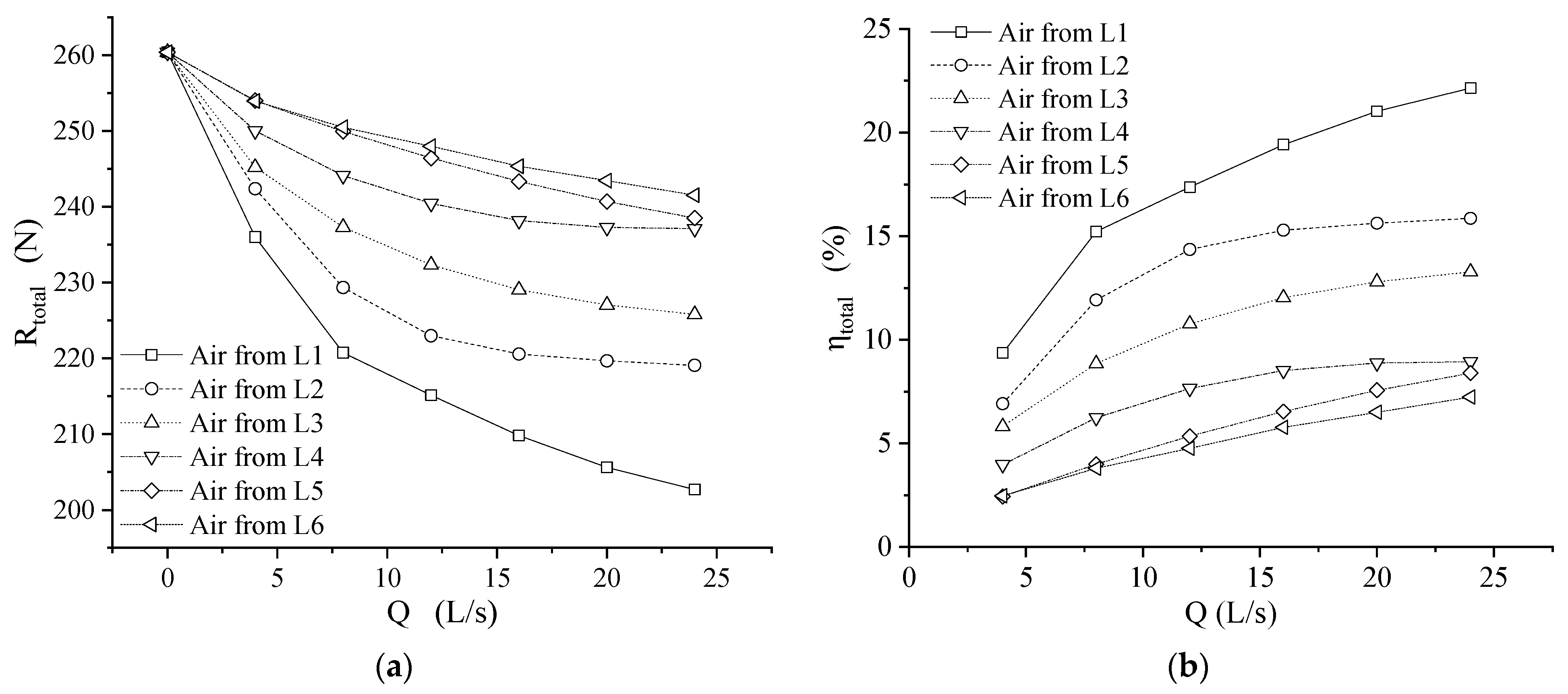
It could be seen that the air injection location has a significant influence on the total resistance, as shown in Figure 6a. The injection location on the underwater body will result in a smaller total resistance than the injection location on the strut. The air injection from the location closer to the front end of SWATH will lead to the lower total resistance. As the airflow rate increases, the resistance gradually decreases, no matter which location the air is injected. In the cases of the air injected from locations L2, L3, and L4, the total resistance curve tends to be stable, and the airflow reaches a saturation rate of 20 L/s. In the cases of injecting air from location L1, even if the airflow rate reaches 24 L/s, the resistance curve still has a downward trend. It is because the injection location L1 is located at the front end of the underwater body. The air could cover a larger surface area, so the saturated airflow rate is more significant than in other cases. It could be seen that the air injected from location L1 will cause the most significant drag reduction, as shown in Figure 6b. When the airflow rate is 24 L/s, the drag reduction can reach 22.15%. The air injected from the location closest to the head of SWATH will lead to a more significant drag reduction. The air injection location on the underwater body is more conducive to drag reduction than the air injection location on the strut.

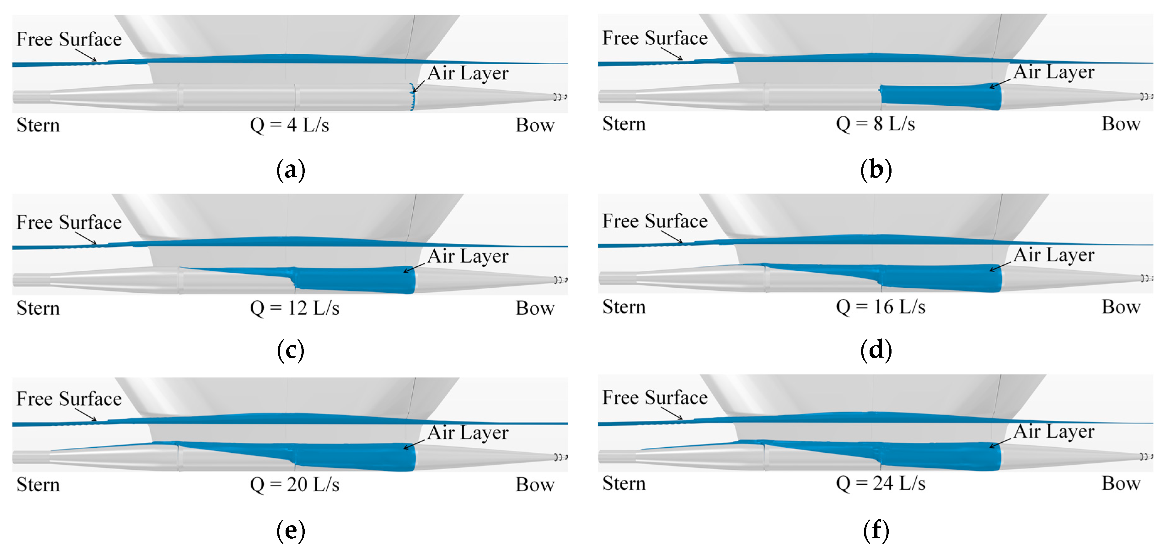
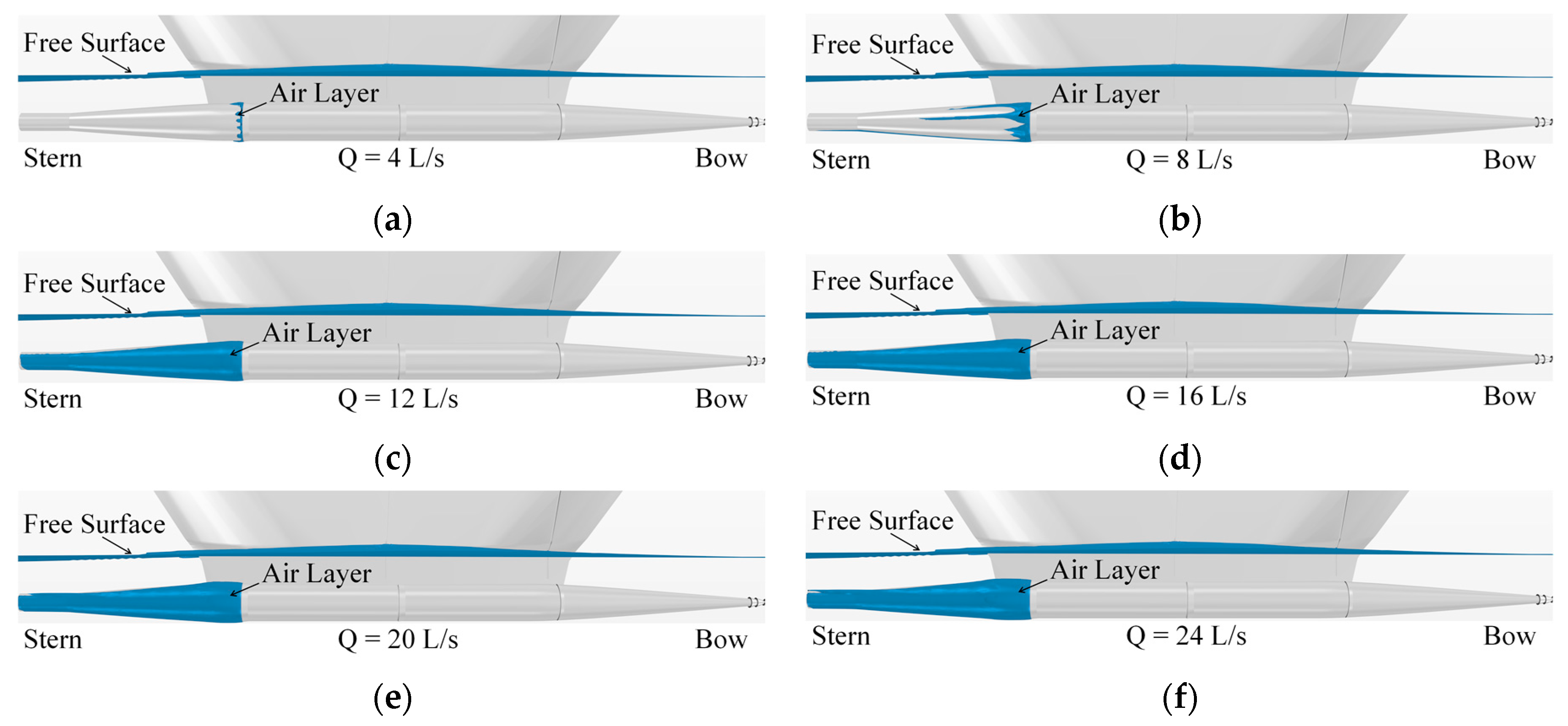
The air layer distribution under different injection locations and airflow rates are shown in Figure 7, Figure 8, Figure 9, Figure 10, Figure 11 and Figure 12. The blue area is the air-water boundary surface with an air volume fraction of 0.5.

By comparing Figure 7a–f, the airflow rate significantly affects the air layer distribution. With a slight airflow rate, Q = 4 L/s, the air layer could only cover the area near injection location L1, as shown in Figure 7a. With the increase in airflow rate, the size of the air layer distribution increases. When the airflow rate is 8 L/s and 12 L/s, the air layer could cover area A1, as shown in Figure 7b,c. As the airflow rate continues to increase, the air layer spreads to the middle of the underwater body, and due to the influence of buoyancy, the air layer covers the upper part of the underwater body, as shown in Figure 7d–f. It could be found that, even with a significant airflow rate, increasing the airflow rate could still increase the area of the air layer distribution.

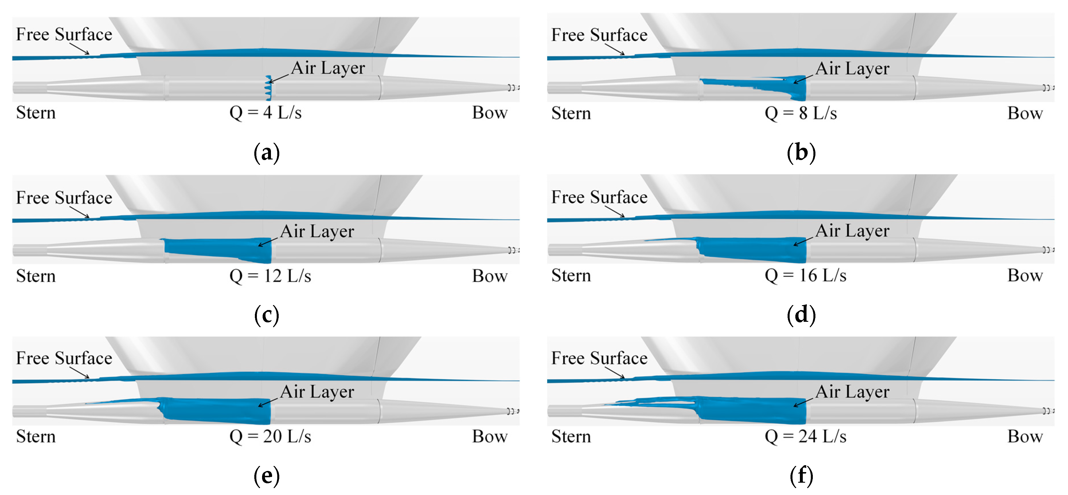
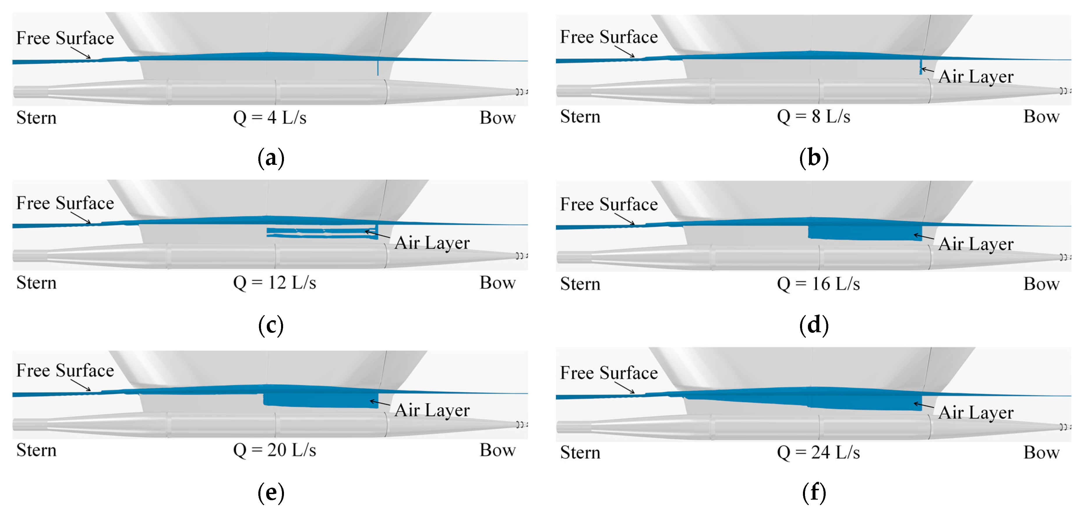
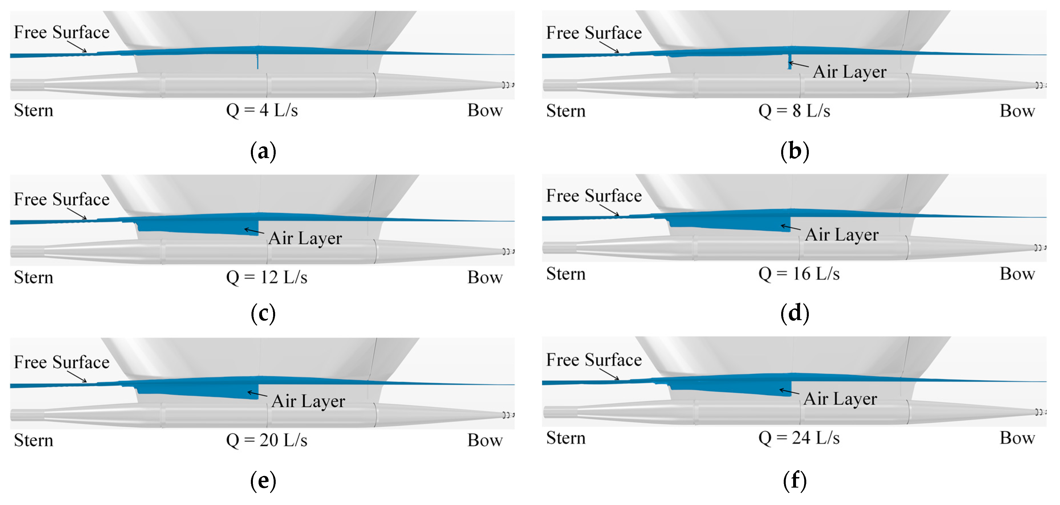
A similar phenomenon can be seen in Figure 8, Figure 9 and Figure 10. The area of the air layer distribution increases with the increase in the airflow rate until the airflow rate reaches 12 L/s. When the airflow rate is more significant than 12 L/s, the difference in the air layer distribution is little.

Figure 11 and Figure 12 show the air layer distribution with air injected from locations L5 and L6, which are set on the strut. It could be seen that, even if the airflow rate reaches 8 L/s, the air layer still could not be effectively covered, as shown in Figure 11a,b and Figure 12a,b. Comparing Figure 11c and Figure 12c, with the medium airflow rate, the air layer distribution of L6 is better than L5, and it is because that location L5 is set at the front side of the strut, which is harmful to the air layer distribution. When the airflow rate increase from 16 L/s to 20 L/s, the air layer distribution has not changed much, as shown in Figure 11e,f and Figure 12e,f. When the airflow rate increase to 24 L/s, the air layer area of L5 increases while the air layer area of L6 still has not changed much, as shown in Figure 11f and Figure 12f.

The air layer varies with different injection locations. The covering of the air layer will affect the performance of appendages, such as foils. According to the analysis of the calculated results, the air layer is thin. The coverage of the air layer mainly changes the fluid density around the area where the fins are connected with the hull surface, which will probably lead to a lifting loss. This paper mainly analyzes the air layer distribution under different injection locations and the airflow rates. So, the corresponding influence on the foils is not included in this paper.

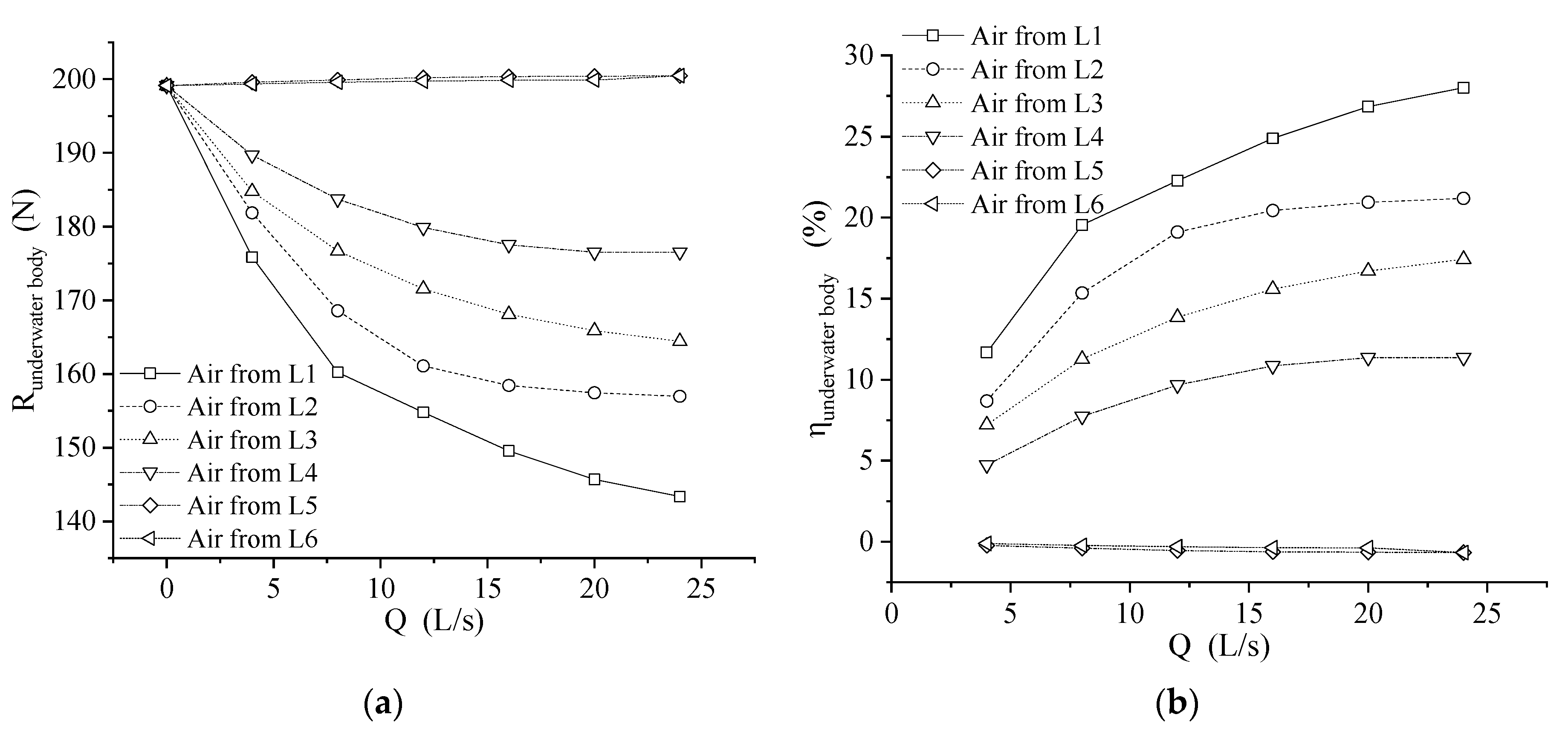
4.2. Effect on the Underwater Body and the Strut

The computed result of resistance and drag reduction in the underwater body is shown in Figure 13. $R_{underwater body}$ is the resistance of the underwater body. ${\eta }_{total}$ is the resistance reduction rate of underwater body.

By Figure 13, it could be found that the air injected from locations L5 and L6, which are on the strut, has a more negligible effect on the resistance and the drag reduction in the underwater body. It is because the air injected from the location on the strut has a tendency to the free surface under the effect of buoyancy. It could be seen that the air injected from the location which is closer to the head of the underwater body will lead to more negligible resistance and more significant drag reduction. It is because the air injected will diffuse along the surface of the underwater body in the opposite direction of the forward hull speed. It will reduce the resistance by covering the surface area in the air layer and the gas-water mixed layer. The closer the injection location is to the head, the larger the hull surface area that could be covered, which will lead to more negligible underwater body resistance and a more significant drag reduction in the underwater body.

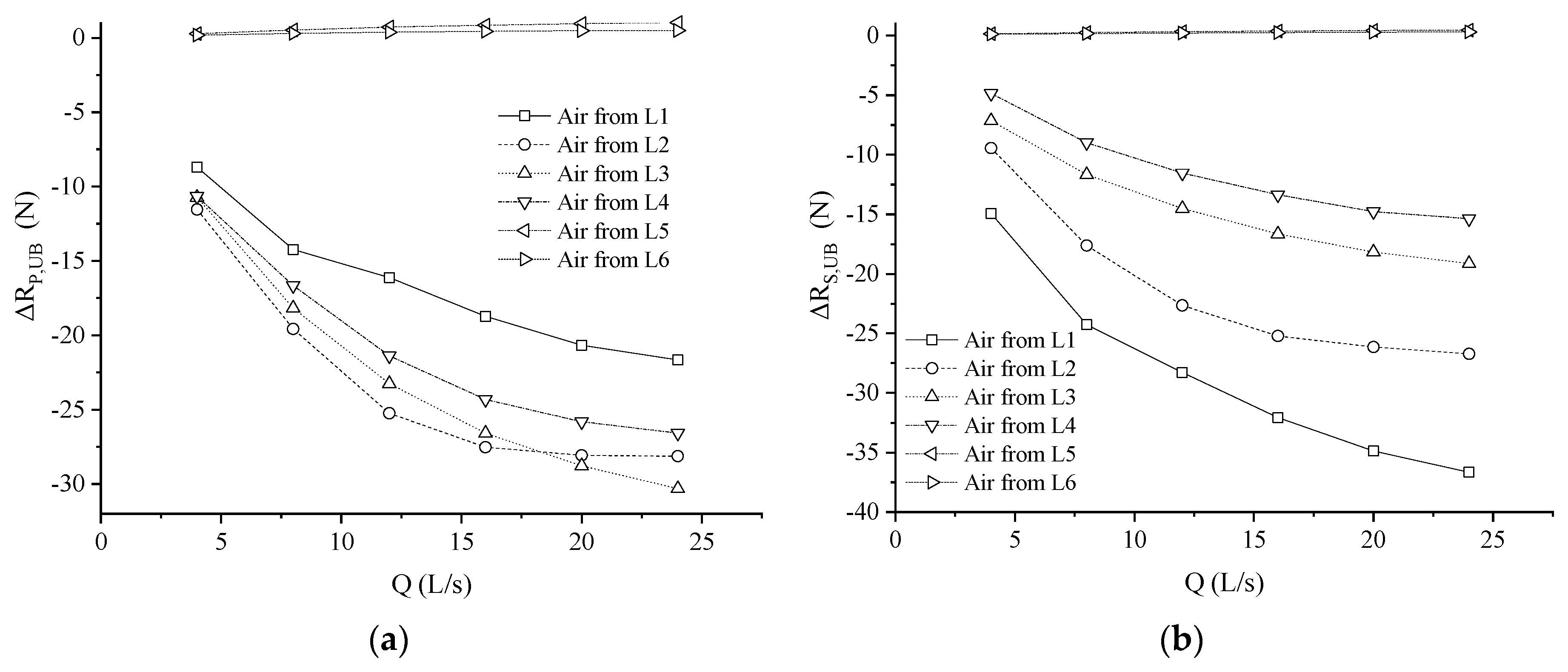
The changes in resistance components before and after air injection are shown in Figure 14. Where $\Delta R_{S,UB}=R_{S,UB}^A-R_{S,UB}^{NA}$, ${\mathrm{R}}_{\mathrm{S},\mathrm{UB}}$ is the resistance component related to the shear force of the underwater body, $R_{S,UB}^A$ is the $R_{S,UB}$ with the air injection, $R_{S,UB}^{NA}$ is the ${\mathrm{R}}_{\mathrm{S},\mathrm{UB}}$ without the air injection. $\Delta R_{P,UB}=R_{P,UB}^A-R_{P,UB}^{NA}$, $R_{P,UB}$ is the resistance component related to the pressure force of the underwater body, $R_{P,UB}^A$ is the $R_{P,UB}$ with the air injection, $R_{P,UB}^{NA}$ is the $R_{P,UB}$ without the air injection.

By Figure 14, it could be found that the air injected from locations L5 and L6 set on the strut, has a negligible effect on the $\Delta R_{P,UB}$ and the $\Delta R_{S,UB}$. When the air injected from the locations L1, L2, L3, and L4 set on the underwater body, the $\Delta R_{P,UB}$ and the $\Delta R_{S,UB}$ decreases with the airflow rate. The $R_{P,UB}$ reduce 21.65 N, 28.13 N, 30.31 N, and 26.58 N with the airflow rate of 24 L/s. The $R_{S,UB}$ reduce 36.66 N, 26.71 N, 19.13 N, and 15.38 N with the airflow rate of 24 L/s.

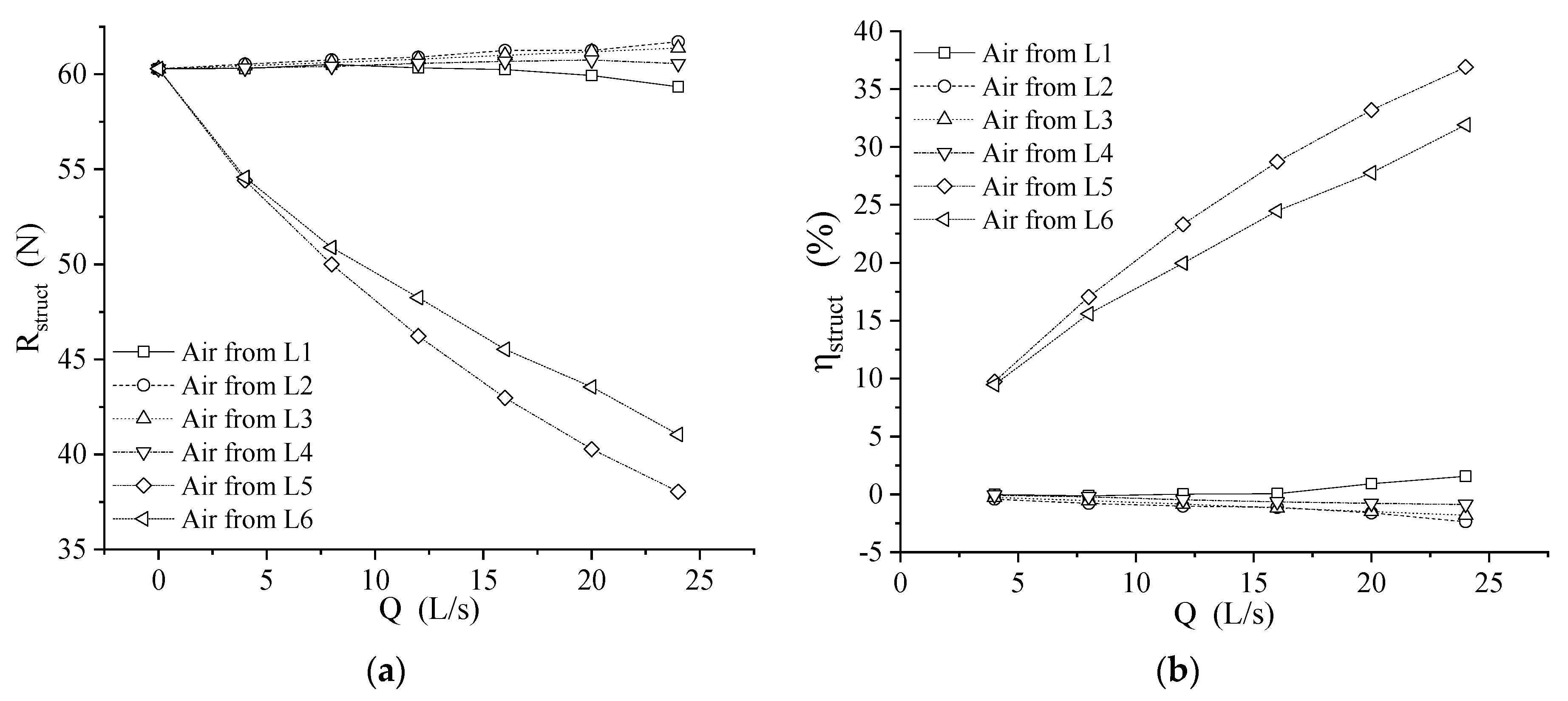
The computed result of resistance and drag reduction in the strut is shown in Figure 15. $R_{strut}$ is the resistance of struts. ${\eta }_{strut}$ is the drag reduction rate of struts.

It could be seen that the air injected from strut locations L5 and L6 has a significant influence on the resistance and the drag reduction in the strut, as shown in Figure 15. The higher airflow rate will lead to more negligible resistance and more significant drag reduction. It could also be noticed that the air injected from location L5 is more conducive to drag reduction than the air injected from location L6. On the airflow rate condition = 24 L/s, the drag reduction in the strut is 36.90% for injection location L5 and 31.92% for injection location L6. It could be found that the air injected from locations L1, L2, L3, and L4 have less influence on the resistance and the drag reduction in the strut for a low airflow rate no larger than 12 L/s. As the airflow rate grows, the resistance of the strut reduces, and the drag reduction in the strut is positive for the air injected from location L1, while the resistance of the strut increases and the drag reduction in the strut is negative.

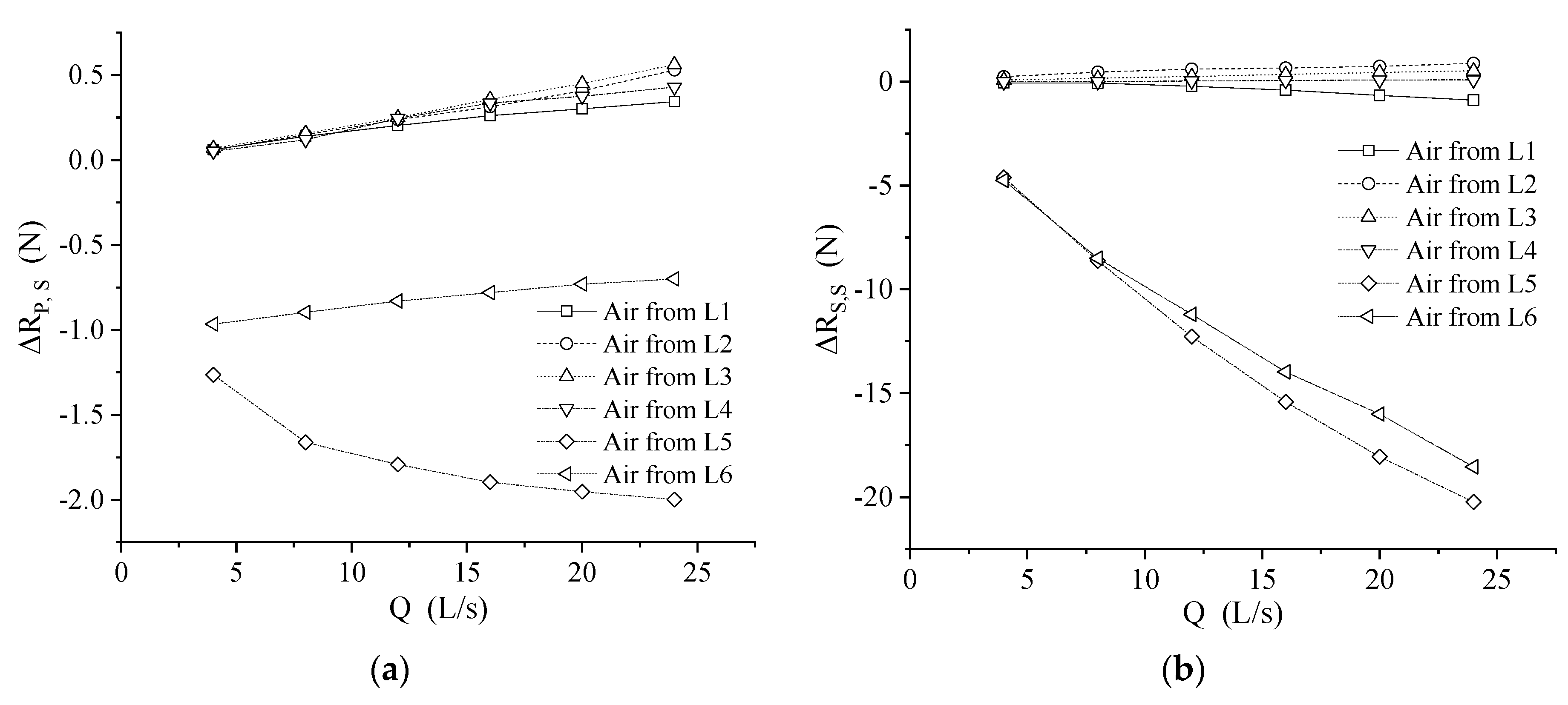
The total resistance has been discussed, and STAR CCM+ software provides a method of measuring resistance components, including $R_S$ and $R_P$, where $R_S$ is the resistance component related to the shear force, which could reflect the friction resistance, and $R_P$ is the resistance component related to the pressure force, which could reflect the viscous pressure resistance and wave resistance. Thus, the changes in resistance components before and after air injection are measured to analyze the cause of the harmful drag reduction in the strut, as shown in Figure 16. Where $\Delta R_{S,S}=R_{S,S}^A-R_{S,S}^{NA}$, $R_{S,S}$ is the resistance component related to the shear force of the strut, $R_{S,S}^A$ is the $R_{S,S}$ with the air injection, $R_{S,S}^{NA}$ is the $R_{S,S}$ without the air injection. $\Delta R_{P,S}=R_{P,S}^A-R_{P,S}^{NA}$, $R_{P,S}$ is the resistance component related to the pressure force of the strut, $R_{P,S}^A$ is the $R_{P,S}$ with the air injection, $R_{P,S}^{NA}$ is the $R_{P,S}$ without the air injection.

It could be seen that when the air was injected from location L5, $\Delta R_{P,S}$ is <0 N and decreases as the airflow rate grows, as shown in Figure 16a. It means that the air injected from location L5 will reduce the resistance component related to the pressure force of the strut, and the decrease is positive as the airflow rate increases. When the air is injected from location L6, $\Delta R_{P,S}$ is also <0 N, but $\Delta R_{P,S}$ will increase as the airflow rate grow, as shown in Figure 16a. It means that the air injected from location L6 will reduce the resistance component related to the pressure force of the strut, but the decrease is negative as the airflow rate increases. The reason is that location L6 is arranged in the middle of the strut, the airflow could reduce the resistance component related to the pressure force of the area behind location L6, but with the airflow injected, the pressure distribution of the area at the front of location L6 will change, and the pressure will increase. With the airflow rate increasing, the influence of the airflow on the area at the front of location L6 gradually increases, which leads to $\Delta R_{P,S}$ increasing as the airflow rate grows. It could be forecast that with the airflow rate continuing to increase, the $\Delta R_{P,S}$ will be a positive value. It could be seen that, $\Delta R_{P,S}$ is > 0 N and increases as the airflow rate grows when the air is injected from locations L1, L2, L3, and L4, as shown in Figure 16a. It means that the air injected from the location on the underwater body will increase the resistance component related to the pressure force of the strut. It also could be noticed that, for the airflow rate > 12 L/s, $\Delta R_{P,S}$ is most significant with the air injected from location L3 and is the slightest with the air injected from location L1, as shown in Figure 17a. The longitudinal location of the injection location on the underwater body influences the resistance component related to the pressure force of the strut, and the closer the injection location is to the middle will lead to the more significant resistance component of the pressure force. By Figure 16b, it can be seen that when the air was injected from the locations L5 and L6, $\Delta R_{S,S}$ are < 0 N and decrease as the flow rate grows. When the airflow rate is ≦8 L/s, there is not much difference between the $\Delta R_{S,S}$ of location L5 and L6. When the airflow rate is >8 L/s, $\Delta R_{S,S}$ of location L5 is smaller than location L6. It means that the airflow injected from location L5 has a greater effect on the resistance component related to the sheer force of the strut than the air injected from location L6. $\Delta R_{S,S}$ is > 0 N and increases as the airflow rate grows when the air is injected from the locations L2, L3, and L4, while $R_{S,S}$ is negative and decreases as the airflow rate grows for the air injected from location L1. By Figure 16, it could be found that the air injected from the locations L2, L3, and L4 has a negative influence on the drag reduction in the strut, which could also be seen in Figure 15.

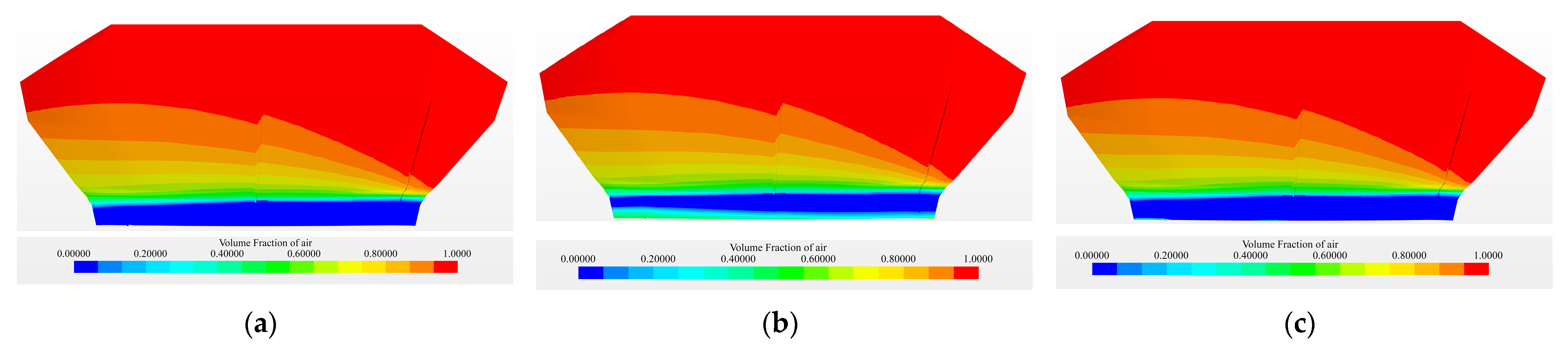
The volume fractions of air of the strut are shown in Figure 17, in which the different colors represent different volume fractions of air. In the dark red area, the volume fraction of air $=$ 1, while the volume fraction of air $=$ 0 in the dark blue area. The yellow area is the water splash range. By Figure 17, it can be seen that the air injected from location L1 could increase the air volume fraction of the bottom of the strut, which is the reason for the negative $\Delta R_{S,S}$, as shown in Figure 16b. By Figure 17, it can be seen that the air injected from location L3 could increase the height of the water splash effect, which is the reason for the positive $\Delta R_{S,S}$, as shown in Figure 16b.

4.3. Effect on the Different Areas of the Underwater Body

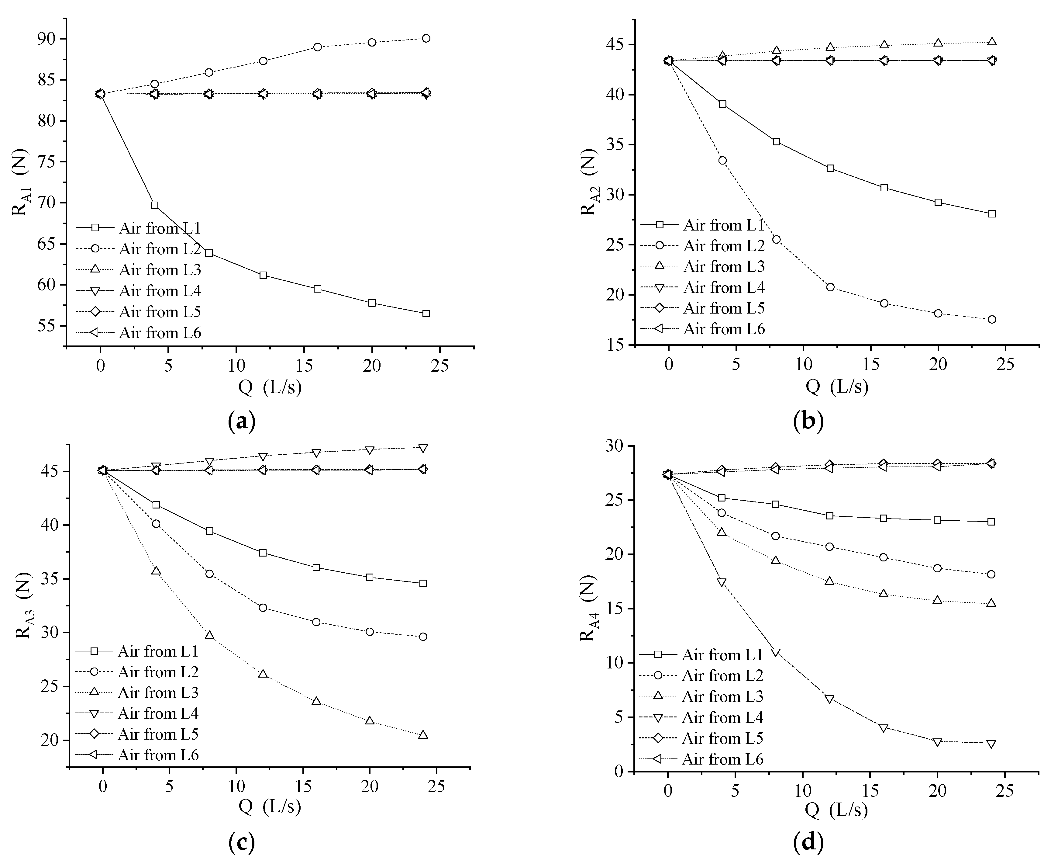
The computed result of resistance and drag reduction in different areas of the underwater body is shown in Figure 18.

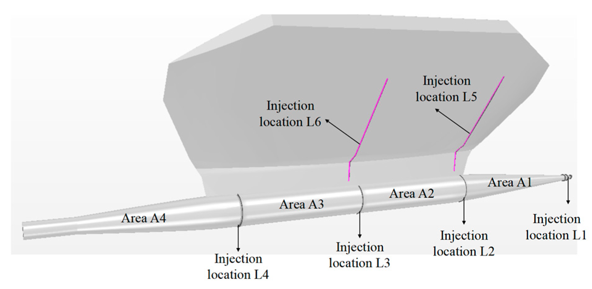
The areas of the underwater body can be seen in Figure 3. It could be noticed that the resistance of a particular area of the underwater body is most affected by the forward injection location, which is nearest to it, as shown in Figure 18. The most negligible resistance of A2, A3, and A4 appear separately when the air is injected from injection locations L2, L3, and L4. 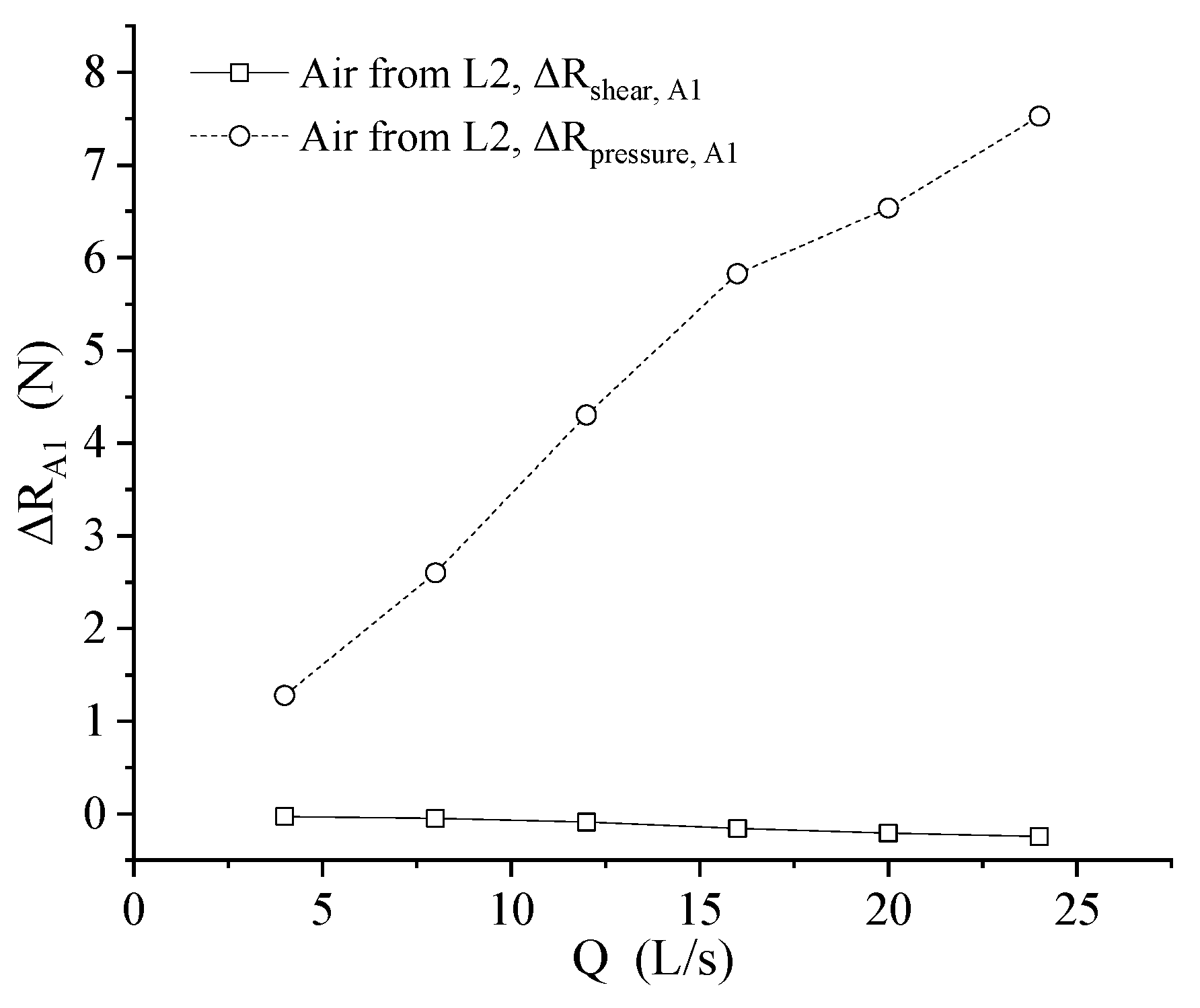It could also be found that the resistance of a particular area will increase when the air is injected from the backward injection location which is nearest to it, as shown in Figure 18. For example, when the air is injected from location L2 with the airflow rate of 12 L/s, the resistance of A1 increases by 7.21 N. The changes of $\Delta R_{shear, A1}$ and $\Delta R_{pressure, A1}$ with the air injected from L2 is shown in Figure 19.

It could be seen that $\Delta R_{pressure, A1}$ is positive and increases with the airflow rate while $\Delta R_{pressure, A1}$ is still close to 0, as shown in Figure 19. It means that the air injected from location L2 will increase the resistance component related to the pressure force of A1. The higher airflow rate will lead to a more significant resistance component related to the pressure force. It could notice that the airflow injected from location L2 cannot cover area A1, as shown in Figure 8, but the airflow could change the pressure distribution of area A1. That is the reason that $\Delta R_{pressure, A1}$ is positive and increases with increasing the airflow rate of location L2, while $\Delta R_{shear, A1}$ is negligibly affected by the airflow. 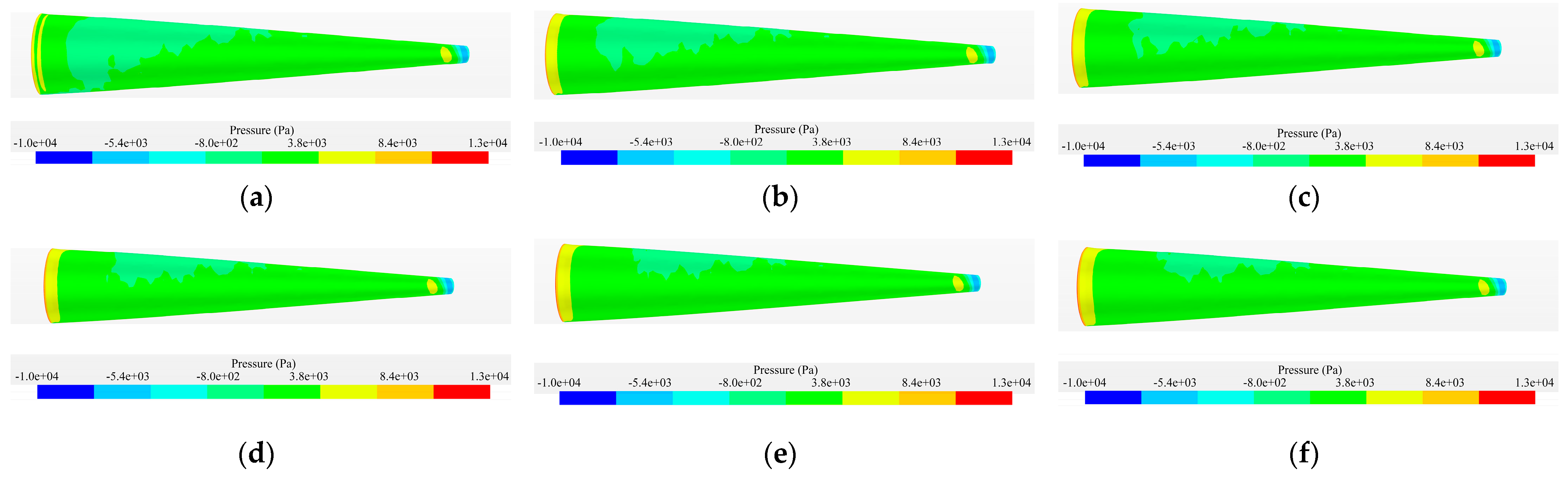Figure 20 shows the pressure distribution of A1 with the air injected from location L2, which could explain the reason for the rising $\Delta R_{pressure, A1}$ phenomenon. It can be seen that the area near the injection location L2 is a high-pressure area, and the pressure in most areas of A1 is between −800 Pa and 3800 Pa, as shown in Figure 20. As the flow rate increases, the area with pressure between −800 Pa and 1500 Pa decreases, and the area with pressure between 1500 Pa and 3800 Pa increases. Besides, the high-pressure area near the injection location L2 increases, too. It means that the overall pressure of area A1 increases with the airflow rate, which is the reason that $\Delta R_{pressure, A1}$ is positive and increases with the airflow rate, as shown in Figure 19.

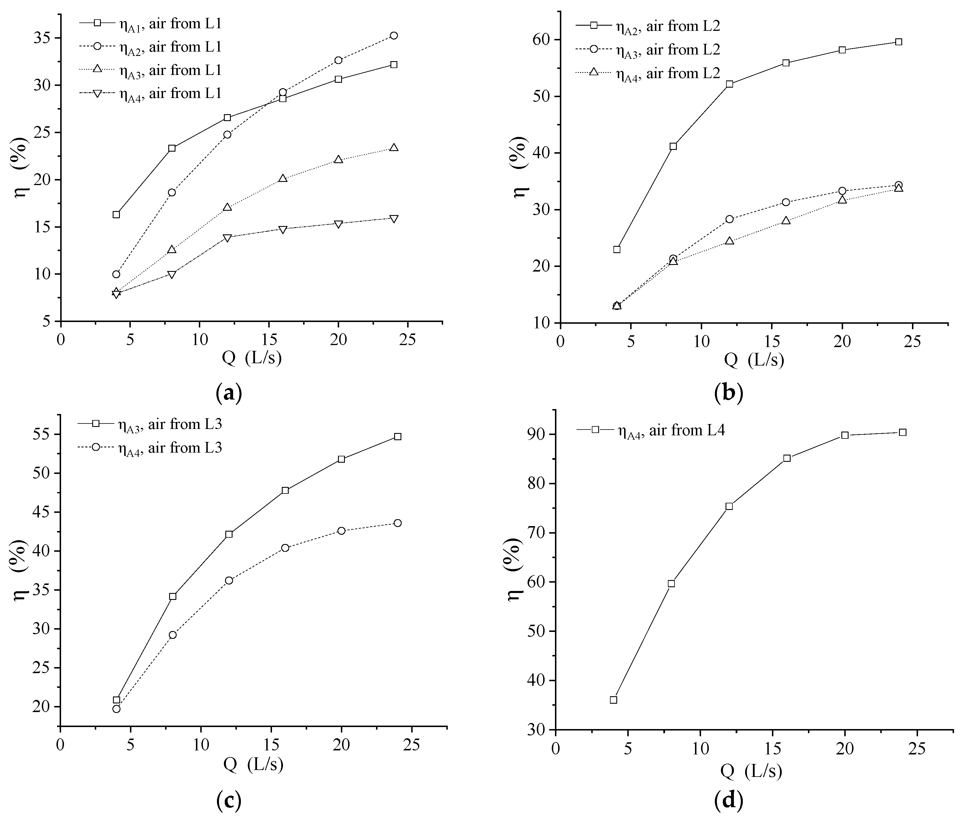
Figure 21 shows the drag reduction in different underwater areas at various airflow rates with other air injection locations. $\eta$ is the drag reduction in different underwater areas, where ${\eta }_{A1}$, ${\eta }_{A2}$, ${\eta }_{A3}$ and ${\eta }_{A4}$ is the drag reduction in A1, A2, A3 and A4, respectively. It could be seen that, with the air injected from L1, the drag reduction in A1 is the largest for the airflow rate ≤ 12 L/s, while the drag reduction in A2 is the largest for the airflow rate ≥ 16 L/s, as shown in Figure 21a. It could be noticed that the most considerable drag reduction in different areas has a significant difference. The drag reduction in A4, which is in the stern area of the underwater body, could reach 90%. The drag reduction in A2 and A3, which are in the middle area of the underwater body, could obtain 50%. The drag reduction in A1, which is in the bow area of the underwater body, could reach 30%. It probably means that there are significant differences in the drag reduction effect of air injection on each area of the underwater body. The stern area has the best impact, and the middle area and the bow area have the worst effect.

5. Conclusions

In this paper, the numerical method of air lubrication is validated. The result shows that the current process can be used to simulate the resistance of SWATH in a numerical calm water tank with airflow injection. Then, the numerical methods are used to predict the resistance of SWATH in calm water and headings at a speed of 8 m/s under different injection locations and airflow rates, and the effect of injection location on SWATH drag reduction is investigated. The numerical results of the cases considered for systemic investigation in the paper indicate the following interesting observations.

Firstly, by analyzing the resistance and drag reduction in SWATH, it is found that the injection location on the underwater body is more conducive to the drag reduction in the SWATH than the injection location on the strut. The most significant drag reduction is 22.15% when the injection location is on the underwater body, and the most significant drag reduction is 8.39% when the injection location is on the strut. Besides, the closer the injection location is to the bow, the better the drag reduction effect.

Secondly, the influence of injection locations on the resistance and drag reduction in the underwater body and the strut is studied. The results show that the injection location on the strut has little effect on the resistance of the underwater body, and the drag reduction effect is negligible. The air injected from locations on the underwater body causes the pressure resistance component of the strut to increase. The air injected from the middle of the underwater body increases the splash range inside the strut and increases the shear resistance component of the strut.

Thirdly, the influence of the injection location on the drag reduction in different areas of the underwater body is analyzed. The results show that, for the area in the front of the injection location, because the airflow changes the pressure distribution in this area, the resistance increases, and the pressure resistance component increases. When the air is injected from the injection location L2, the resistance in the A1 area increases by 8.14%, and the pressure resistance component increases by 12.83%. Besides, there are significant differences in drag reduction effects in different areas. The drag reduction in the area near the bow is higher than that of the area located at the middle part and near the stern.

References

1. Subramanian, V.A.; Beena, V.I. Numeric design and evaluation of swath form. Int. Shipbuild. Prog. 2002, 49, 95–125. [Google Scholar]
2. McNatt, T.; Ma, M. Historical perspective on the structural design of special ships and the evolution of structural design methods. Ships Offshore Struct. 2013, 8, 404–414. [Google Scholar] [CrossRef]
3. Vernengo, G.; Brizzolara, S. Numerical investigation on the hydrodynamic performance of fast SWATHs with optimum canted struts arrangements. Appl. Ocean Res. 2017, 63, 76–89. [Google Scholar] [CrossRef] [Green Version]
4. Brizzolara, S. Parametric optimization of SWAT-Hull forms by a viscous-inviscid free surface method driven by a differential evolution algorithm. In Proceedings of the 25th Symposium on Naval Hydrodynamics, Saint John’s, NL, Canada, 8–13 August 2004; National Academies Press: Washington, DC, USA, 2004; Volume 5, pp. 1–18. [Google Scholar]
5. Qian, P.; Yi, H.; Li, Y. Numerical and experimental studies on hydrodynamic performance of a small-waterplane-area-twin-hull (swath) vehicle with inclined struts. Ocean Eng. 2015, 96, 181–191. [Google Scholar] [CrossRef]
6. Lin, Y.; Yang, Q.; Guan, G. Automatic design optimization of SWATH applying CFD and RSM model. Ocean Eng. 2019, 172, 146–154. [Google Scholar] [CrossRef]
7. Jang, J.; Choi, S.H.; Ahn, S.-M.; Kim, B.; Seo, J.S. Experimental investigation of frictional resistance reduction with air layer on the hull bottom of a ship. Int. J. Nav. Archit. Ocean Eng. 2014, 6, 363–379. [Google Scholar] [CrossRef] [Green Version]
8. Butterworth, J.; Atlar, M.; Shi, W. Experimental analysis of an air cavity concept applied on a ship hull to improve the hull resistance. Ocean Eng. 2015, 110, 2–10. [Google Scholar] [CrossRef] [Green Version]
9. Matveev, K.I. Hydrodynamic modeling of semi-planing hulls with air cavities. Int. J. Nav. Archit. Ocean Eng. 2015, 7, 500–508. [Google Scholar] [CrossRef] [Green Version]
10. Cucinotta, F.; Guglielmino, E.; Sfravara, F.; Strasser, C. Numerical and experimental investigation of a planing Air Cavity Ship and its air layer evolution. Ocean Eng. 2018, 152, 130–144. [Google Scholar] [CrossRef]
11. Wu, H. Numerical study of the effect of ship attitude on the perform of ship with air injection in bottom cavity. Ocean Eng. 2019, 186, 106119. [Google Scholar]
12. Wu, H.; Ou, Y. Experimental study of air layer drag reduction with bottom cavity for a bulk carrier ship model. China Ocean Eng. 2019, 5, 554–562. [Google Scholar] [CrossRef]
13. Wu, H.; Ou, Y. Analysis of air layer shape formed by air injection at the bottom of flat plate. Ocean Eng. 2020, 216, 108091. [Google Scholar] [CrossRef]
14. Elbing, B.R.; Winkel, E.S.; Lay, K.A.; Ceccio, S.L.; Dowling, D.R.; Perlin, M. Bubble-Induced Skin-Friction drag reduction and the abrupt transition to Air-Layer drag reduction. J. Fluid Mech. 2008, 612, 201–236. [Google Scholar] [CrossRef]
15. Murai, Y.; Fukuda, H.; Oishi, Y.; Kodama, Y.; Yamamoto, F. Skin friction reduction by large air bubbles in a horizontal channel flow. Int. J. Multiph. Flow 2007, 33, 147–163. [Google Scholar] [CrossRef]
16. Murai, Y. Frictional drag reduction by bubble injection. Exp. Fluid. 2014, 55, 1773. [Google Scholar] [CrossRef]
17. Slyozkin, A.; Atlar, M.; Sampson, R.; Seo, K.C. An experimental investigation into the hydrodynamic drag reduction of a flat plate using air-fed cavities. Ocean Eng. 2014, 76, 105–120. [Google Scholar] [CrossRef]
18. Amromi, E.L. Analysis of interaction between ship bottom air cavity and boundary layer. Appl. Ocean Res. 2016, 59, 451–458. [Google Scholar] [CrossRef]
19. Elbing, B.R.; Mäkiharju, S.; Wiggins, A.; Perlin, M.; Dowling, D.R.; Ceccio, S.L. On the scaling of air layer drag reduction. J. Fluid Mech. 2013, 717, 484–513. [Google Scholar] [CrossRef]
20. Makiharju, S.; Ceccio, S. On multi-point gas injection to form an air layer for frictional drag reduction. Ocean Eng. 2018, 147, 206–214. [Google Scholar] [CrossRef]
21. Pearce, B.W.; Brandner, P.A.; Foster, S.J. Ventilated cavity flow over a backward-facing step. Phys. Conf. Ser. 2015, 656, 012164. [Google Scholar] [CrossRef] [Green Version]
22. Cucinotta, F.; Guglielmino, E.; Sfravara, F. An experimental comparison between different artificial air cavity designs for a planing hull. Ocean Eng. 2017, 140, 233–243. [Google Scholar] [CrossRef]
23. Schlichting, H.; Kestin, J. Boundary Layer Theory; McGraw-Hill: New York, NY, USA, 1961. [Google Scholar]
24. Stern, F.; Wilson, R.V.; Coleman, H.W.; Paterson, E.G. Comprehensive approach to verification and validation of CFD simulations-part 1: Methodology and procedures. J. Fluids Eng. 2001, 123, 793–802. [Google Scholar] [CrossRef]
25. Wilson, R.V.; Stern, F.; Coleman, H.W.; Paterson, E.G. Comprehensive approach to verification and validation of CFD simulations—Part 2: Application for RANS simulation of a cargo/container ship. J. Fluids Eng. 2001, 123, 803–810. [Google Scholar] [CrossRef]
Figure 1. Computational domain and mesh: (a) Computational domain and boundaries; (b) Mesh for the domain.
Jmse 11 00667 g001
Figure 2. Geometry model of the SWATH.
Jmse 11 00667 g002
Figure 3. Air injection locations and areas.
Jmse 11 00667 g003
Figure 4. Experimental setup for model tests.
Jmse 11 00667 g004
Figure 5. The total resistance R total . .
Jmse 11 00667 g005
Figure 6. Resistance and drag reduction in SWATH with different air injection locations: (a) Total resistance; (b) Drag reduction.
Jmse 11 00667 g006
Figure 7. Air layer distribution with air injected from location L1: (a) Airflow rate Q = 4 L/s; (b) Airflow rate Q = 8 L/s; (c) Airflow rate Q = 12 L/s; (d) Airflow rate Q = 16 L/s; (e) Airflow rate Q = 20 L/s; (f) Airflow rate Q = 24 L/s.
Jmse 11 00667 g007
Figure 8. Air layer distribution with air injected from location L2: (a) Airflow rate Q = 4 L/s; (b) Airflow rate Q = 8 L/s; (c) Airflow rate Q = 12 L/s; (d) Airflow rate Q = 16 L/s; (e) Airflow rate Q = 20 L/s; (f) Airflow rate Q = 24 L/s.
Jmse 11 00667 g008
Figure 9. Air layer distribution with air injected from location L3: (a) Airflow rate Q = 4 L/s; (b) Airflow rate Q = 8 L/s; (c) Airflow rate Q = 12 L/s; (d) Airflow rate Q = 16 L/s; (e) Airflow rate Q = 20 L/s; (f) Airflow rate Q = 24 L/s.
Jmse 11 00667 g009
Figure 10. Air layer distribution with air injected from location L4: (a) Airflow rate Q = 4 L/s; (b) Airflow rate Q = 8 L/s; (c) Airflow rate Q = 12 L/s; (d) Airflow rate Q = 16 L/s; (e) Airflow rate Q = 20 L/s; (f) Airflow rate Q = 24 L/s.
Jmse 11 00667 g010
Figure 11. Air layer distribution with air injected from location L5: (a) Airflow rate Q = 4 L/s; (b) Airflow rate Q = 8 L/s; (c) Airflow rate Q = 12 L/s; (d) Airflow rate Q = 16 L/s; (e) Airflow rate Q = 20 L/s; (f) Airflow rate Q = 24 L/s.
Jmse 11 00667 g011
Figure 12. Air layer distribution with air injected from location L6: (a) Airflow rate Q = 4 L/s; (b) Airflow rate Q = 8 L/s; (c) Airflow rate Q = 12 L/s; (d) Airflow rate Q = 16 L/s; (e) Airflow rate Q = 20 L/s; (f) Airflow rate Q = 24 L/s.
Jmse 11 00667 g012
Figure 13. Resistance and drag reduction in the underwater body with different air injection locations: (a) Total resistance; (b) Drag reduction.
Jmse 11 00667 g013
Figure 14. Changes in the resistance component of the underwater body: (a) Component related to the pressure force; (b) Component related to the shear force.
Jmse 11 00667 g014
Figure 15. Resistance and drag reduction in the strut with different air injection locations: (a) Total resistance; (b) Drag reduction.
Jmse 11 00667 g015
Figure 16. Changes in the resistance component of the strut: (a) Component related to the pressure force; (b) Component related to the shear force.
Jmse 11 00667 g016
Figure 17. Volume fraction of air of the strut: (a) Without air injection; (b) Injected from L1, Airflow rate = 24 L/s; (c) Injected from L3, Airflow rate = 24 L/s.
Jmse 11 00667 g017
Figure 18. Resistance of different areas of the underwater body: (a) Total resistance of A1; (b) Total resistance of A2; (c) Total resistance of A3; (d) Total resistance of A4.
Jmse 11 00667 g018
Figure 19. Changes in the resistance component of A1 with the air injected from location L2.
Jmse 11 00667 g019
Figure 20. Pressure distribution of A1 with the air injected from the location L2: (a) Without air injection; (b) Airflow rate Q = 8 L/s; (c) Airflow rate Q = 12 L/s; (d) Airflow rate Q = 16 L/s; (e) Airflow rate Q = 20 L/s; (f) Airflow rate Q = 24 L/s.
Jmse 11 00667 g020
Figure 21. Drag reduction in the underwater areas with different air injection locations: (a) Air injected from L1; (b) Air injected from L2; (c) Air injected from L3; (d) Air injected from L4.
Jmse 11 00667 g021