Article

Optimization Study of Marine Energy Harvesting from Vortex-Induced Vibration Using a Response-Surface Method

1
School of Naval Architecture and Maritime, Zhejiang Ocean University, Zhoushan 316022, China
2
Institute of Ship Technology and Ocean Engineering, University of Duisburg-Essen, 47057 Duisburg, Germany
*
Author to whom correspondence should be addressed.
J. Mar. Sci. Eng. 2023, 11(3), 668; https://doi.org/10.3390/jmse11030668
Submission received: 18 February 2023 / Revised: 18 March 2023 / Accepted: 19 March 2023 / Published: 22 March 2023
(This article belongs to the Special Issue Advanced Marine Energy Harvesting Technologies)

Abstract

:
Vortex-induced vibration (VIV) of bluff bodies is one type of flow-induced vibration phenomenon, and the possibility of using it to harvest hydrokinetic energy from marine currents has recently been revealed. To develop an optimal harvester, various parameters such as mass ratio, structural stiffness, and inflow velocity need to be explored, resulting in a large number of test cases. This study primarily aims to examine the validity of a parameter optimization approach to maximize the energy capture efficiency using VIV. The Box–Behnken design response-surface method (RSM-BBD) applied in the present study, for an optimization purpose, allows for us to efficiently explore these parameters, consequently reducing the number of experiments. The proper combinations of these operating variables were then identified in this regard. Within this algorithm, the spring stiffness, the reduced velocity, and the vibrator diameter are set as level factors. Correspondingly, the energy conversion efficiency was taken as the observed value of the target. The predicted results were validated by comparing the optimized parameters to values collected from the literature, as well as to our simulations using a computational-fluid dynamics (CFD) model. Generally, the optimal operating conditions predicted using the response-surface method agreed well with those simulated using our CFD model. The number of experiments was successfully reduced somewhat, and the operating conditions that lead to the highest efficiency of energy harvesting using VIV were determined.

1. Introduction

In recent years, a strong demand has developed for transforming energy supply from fossil fuels towards renewable energy sources, such as solar, wind, and wave. In this context, marine energy, such as ocean currents, offers a significant potential for emissions-free and self-sufficient energy production. Nevertheless, the path to the utilization of currents has been very difficult, as the majority of ocean and river currents are slow, making harvesting of their energy by turbines or watermills challenging [1]. On the other hand, engineered structures with bluff cross-sections, such as circular cylinders and slender structures, may generate alternating or oscillatory lift in uniform flows. As is well known, vortex-induced vibration (VIV) generally occurs to a bluff body immersed in a cross flow, creating shedding vortices in the downstream, with oscillatory unsteady forces, and resulting in an oscillatory motion of the bluff body [2]. Lock-in is an important phenomenon associated with VIV of a bluff body, characterized by a high amplitude of body vibrations. To study the typical determining factors of a single-cylinder VIV, and characterize its lock-in regime, numerous experimental and numerical works have been carried out. For instance, Feng [3] performed wind tunnel experiments to investigate the issue of vortex vibration of a single cylindrical structure and first uncovered the phenomenon of vortex vibration. Khalak and Williamson [4,5] designed an experimental apparatus to study the effect of mass ratio, and the characteristics of the initial branch, the upper branch, and the lower branch, were illustrated using an amplitude graph of the vortex-excited vibrations of a cylindrical structure at different mass ratios. Alternatively, numerical computations are sometimes performed, based on two-dimensional, or more often three-dimensional, assumptions. For instance, Govardhan and Williamson studied VIV and vortex shedding modes using two- and three-dimensional numerical simulations [6,7]. Similarly, Shi et al. [8] studied the influence of corner rounding on the near-wake pattern and vortex structure of a square cylinder flow, by using two- and three-dimensional large eddy simulations. Cravero et al. [9] presented a methodology for the prediction of the recirculation length of the unsteady wake from a bluff body, and the quantitative correlation of higher recirculation length with lower shedding frequency was confirmed for considered applications at different operating conditions. For further works related to synchronization in VIV, see the detailed reviews of [10,11,12]. It is worth noting, that in practical offshore applications, provided that a structure is flexible or flexibly mounted, VIV may cause vibrations, leading to stresses and fatigue damage.
Apart from its drawbacks, on the other hand, recent developments have revealed the possibility of extracting hydrokinetic energy using the VIV phenomena, such as the vortex-induced vibration aquatic clean energy (VIVACE) converter [13]. This converter maximizes the use of VIV energy by enhancing, rather than suppressing, the self-excited vibrations of a cylinder due to its vortex shedding. This concept has been studied extensively since then, consisting of model tests [14], computational fluid dynamics (CFD) [15], and mathematical models [16]. More specifically, a comprehensive physical model study was performed by Narendran et al. [17], to understand the underlying physics behind VIV. Their experimental set-up consisted of a linear generator, which had low mechanical losses, leading to a higher mechanical efficiency. Additionally, they also carried out a detailed parametric investigation, over a wide range of system parameters, such as mass ratio, damping ratio, and Reynolds number, using a new analytical model. Ding et al. [18] numerically studied flow-induced motion and energy harvesting of bluff bodies with different cross-sections, where time-dependent viscous flow solutions were obtained, by combining the incompressible unsteady Reynolds-averaged Navier–Stokes equations, with the Spalart–Allmaras turbulence model. Similarly, energy harvesting via VIV of bluff bodies with different cross-sections in tandem arrangement, was numerically studied by Zhang et al. [19]. Furthermore, Wu et al. [20] studied the VIV of a cylinder at a low Reynolds number, based on CFD simulations, cylinders with eight different gap ratios were considered. The responses of the cylinder system were discussed, following the classification of the flow patterns at different gap ratios. Zhang et al. [21] numerically investigated the effects of the damping-ratio and mass-ratio, on energy harnessing of a square cylinder in flow-induced motion. Their results showed that, as the velocity increased, the number of vortices shed per cycle increased, and the harnessed power increased, without an upper limit. The energy conversion efficiency increased up to the highest value, until the VIV upper branch. In summary, marine current energy may be harvested using one [22] or multiple cylindrical oscillators [23], where smooth cylinders or passive turbulence control could be adopted [24].
To develop an optimal harvester, various parameters such as mass ratio, structural stiffness, and inflow velocity need to be explored, resulting in a large number of test cases. In such contexts, the design-of-experiment (DOE) approach can assist, to perform a systematical and effective analysis [25]. By arranging and interpreting some of the main cases, a DOE approach derives optimal results through a minimum number of analysis cases. As a type of DOE approach, response-surface methodology (RSM) is an optimization method that integrates experimental design and mathematical modeling, to obtain an optimal level of each factor, by fitting the function between the factors and the results in the global range, through experiments at representative local points [26]. Combining optimization methodologies such as an RSM, with numerical models, avoids expensive and time-consuming experiments, while allowing for obtaining optimal conditions using different input combinations. A growing number of studies have adopted an RSM combined with CFD calculations, to identify the dominating factors affecting specific parameters and/or responses, that are vital in field operations. For instance, Seok et al. improved the bow shape of a tanker hull, where CFD simulations were minimized by applying an RSM optimization algorithm [27]. By modeling a dairy building through RSM models and CFD calculations, Yi et al. [28] examined the effects of opening ratio, building length to width ratio, and wind speed, on the air exchange rate. Typically, as an efficient model, with three-level experimental design, Box–Behnken design (BBD) is a practical design method within RSM, that can evaluate the nonlinear relationship between indicators and factors [29]. In comparison to other practical design methods with the same number of elements, BBD has the benefit that it does not necessitate several consecutive trials, which can significantly minimize the number of tests. This optimization method has been successfully applied in various engineering branches [30,31,32,33,34,35]. Nevertheless, its application in marine engineering has been limited. Specifically, to our best knowledge, an optimization study of marine current energy harvesting from VIV using such an RSM is still missing from the literature.
This study aims to demonstrate the applicability of an RSM optimization working scheme, that helps to maximize the energy capture efficiency using VIV. The adopted BBD optimization algorithm allows for us to efficiently explore various design parameters, as well as their influences on the energy capture efficiency. First, a three-dimensional VIV model is constructed, using the finite-volume method. Its numerical setup and model accuracy are then verified by performing grid and time-step sensitivity studies. The optimization algorithm is then introduced, to build models between the energy capture efficiency and its dominant design parameters, i.e., the spring stiffness, mass ratio, and incoming flow velocity, in the present study. The validity of the adopted BBD algorithm is then examined, by comparing its predictions with results obtained from the literature, as well as from our CFD simulations. Finally, the influences of the considered design parameters are systematically and effectively analyzed. This work lays a meaningful case foundation for the combination of a response-surface methodology and computational-fluid dynamics approach to optimize the efficiency of marine energy harvesting from VIV, demonstrating the effectiveness of our coupled design.

2. Optimization Methodology

This section covers the optimization methodology adopted in the present study. A brief introduction of its basic concept is first given. Its validity is then roughly examined, by comparing its prediction with results collected from the literature [36,37,38]. A systematic verification of the adopted optimization methodology is performed in Section 5, where its predictions are validated against our CFD simulations.

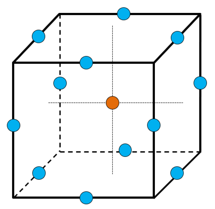
2.1. Concept of Response-Surface Method

Response-surface methodology (RSM) is a computational and scientific technique for modeling and analyzing situations, that considers various factors impacting the desired response and attempts to maximize the result [39]:
y = f x 1 , x 2 + ϵ
Here, variables x 1 and x 2 maximize the yield of a process y. ϵ is the error variable. Its efficiency depends on the accuracy of y at various points throughout the response surface. Box–Behnken design (BBD) is a three-level RSM design, fitting a second-order response-surface model [40,41]:
y = β 0 + i = 1 k β i x i + i = 1 k β i i x i 2 + i < j β i j x i x j + ϵ
where i and j are the linear and quadratic coefficients, respectively. x i and x j are the uncoded independent variables, and k is the number of factors studied and optimized in the experiment. Its parameters β , are estimated by using the least-square approach, where a surface-response analysis is performed on the linked surface.
A BBD requires only the low, middle, and high levels for each design variable. As shown in Figure 1, the levels of factors are at the midpoints of the edges (blue dots), and in the center is the center point (orange dot). It does not account for corner points (i.e., points with design factors at their highest levels), because it tends to avoid extreme settings for experiments, which can potentially lead to higher prediction variance near the vertices [42]. The three-dimensional coordinates of each design point in the figure represent the three test levels of each test point, and the test itself requires that the three levels are equally distributed throughout the domain. N = 2 k × k 1 + C 0 , where k represents the number of factors and C 0 represents the number of central test point, is used to estimate the test error [22].

2.2. Feasibility Verification of Response-Surface Method

To verify the feasibility of the adopted optimization algorithm, before starting our simulations, various operational variables were collected from the literature [38], and their proper combinations are validated against our predictions using BBD in this subsection. The considered verification case consisted of double cylinders with various diameter ratios and spacing ratios. The associated energy capture efficiency was simulated using CFD, for various reduced velocities. In this regard, the cylinders’ diameters, inlet velocities, and spacing ratios between cylinders, were selected as level factors. The associated energy capture efficiencies were treated as target observation, as shown in Figure 2. Herein, a three-dimensional (3D) surface graph allows the correlation between a response variable and two operating variables to be viewed. Furthermore, to determine the influence degrees of the two operating variables on the response value, one may observe the slope of a response surface. The steeper the slope, the more significant the corresponding operating variable is, making it intuitive to find an optimal range of operating variables.
We see that the chosen operating variables (i.e., spacing ratio, diameter ratio, and reduced velocity) all have a significant influence on the response variable (i.e., efficiency). There is a relationship between each of the two operating variables, and their optimal combinations are identified, leading to the maximum response value. Specifically, as shown in Figure 2a, at small diameter ratios, the efficiency increases with the increase in spacing ratio. However, this is not the case for large diameter ratios, where the efficiency decreases with the increase in spacing ratio. The influence of diameter ratio on the efficiency, has more or less the same trend of that of the spacing ratio. The interactions of spacing ratio and diameter ratio with reduced velocity, are given in Figure 2b and Figure 2c, respectively. We see that the efficiencies increase first, and then decrease, as the inlet velocity increases. This is because there was a locking interval of incoming velocity on the vibration energy of the oscillator, and within the locking interval, the motion system reached the maximum energy conversion efficiency. Table 1 lists the energy capture efficiencies collected from the literature under various operating conditions. Meanwhile, the predicted maximum efficiency using the optimal operating conditions is also included, where the spacing ratio is 5.78, diameter ratio is 0.99, and the reduced velocity is 5.23. In such an optimal condition, the corresponding efficiency is 36.10%.
Overall, for all the considered operating variables, the surface curves are steep, indicating that the chosen operating variables within this validation study all have a pronounced influence on the target response variable. From which, one may possibly identify the optimum setting of each operating parameter, leading to the maximum energy capture efficiency. We conclude that the adopted BBD algorithm is feasible in the VIV research area, evidenced by the fact that these peaks in the response surfaces, represent the most significant response values among the factors and levels under study. The maximum efficiency was successfully predicted using the optimal conditions. It must be emphasized that the predicted maximum efficiency was only roughly evaluated against the used input data rather than a systematic comparison against CFD simulations. To verify the correct and reliable application of the present method for VIV, the latter will be addressed in Section 5.

3. Numerical Methods of Modeling Fluid–Structure Interaction

To model the VIV of a single cylinder, the numerical methods used for modeling fluid–structure interaction are addressed in this section. The fluid dynamics is solved using the finite-volume method, while the equation of motion of a rigid body is treated as a classical spring-damper system. They are solved within Star-CCM+, in an implicitly coupled manner.

3.1. Computational Fluid Dynamics

For an incompressible and viscous flow, i.e., water in the present study, it is governed by the continuity and the momentum conservation laws:
· v = 0
v t + v · v = ν 2 v 1 ρ p + g
where v is the fluid velocity filed vector, ν and ρ are the kinematic viscosity and the density field, respectively, p is the pressure, and g is the gravity vector. The force acting on the body is given as follows [43]:
F = F p + F v = S n p d S + S ρ 2 ν 2 n · v + v T d S
where subscripts p and v denote the pressure and viscous component of the fluid-induced force, respectively. n stands for surface normal vector of the body surface.
To solve turbulent flows, the two-equation model K-epsilon [44], was used in this study. This model has been applied to vortex shedding in previous work [45] Consequently, the velocity and pressure may be decomposed into time-averaged values v ¯ , p ¯ , and turbulent fluctuations v , p , the time average of which is zero:
v = v ¯ + v p = p ¯ + p
Inserting Equation (6) into Equations (3) and (4), results in the Reynolds Averaged Navier–Stokes (RANS) equations for incompressible flow. The solution domain is discretized into a finite number of control volumes, which may be of arbitrary shape. Second-order temporal and spatial discretization schemes were adopted. The convergence criterion, which is the residual of velocity components and pressure in the momentum equations, was set to 10 4 .

3.2. Rigid Body Motions

In the Star-CCM+ software, the motion of a rigid body was solved using the dynamic fluid body interaction (DFBI) tool. Considering the transverse motion of an elastically mounted cylinder only, its equation of motion can be simplified as the classical mass-spring-damper oscillator model in one degree of freedom (DOF):
m z ¨ + c z ˙ + k z = F z
where z is the position of the rigid body in the transverse direction, and F z is the corresponding fluid force in that direction. m, c, and k are the structural system mass, damping, and stiffness, respectively. After a dimensionless analysis, the following parameters are introduced:
m * = m m f = 4 m ρ π d 2 l ζ = c 2 k m f n = 1 2 π k m v r = v d f n
where m * is the mass ratio and m f is the mass of fluid occupied by the structure. d and l are the body’s diameter and length, respectively. ζ is the damping ratio and f n is the natural frequency, and v r is the reduced velocity. The drag and lift coefficients are defined as:
c d = 2 F x ρ v 2 d l c l = 2 F z ρ v 2 d l
where v is the free stream velocity, and F x and F z are the drag and lift forces exerted by fluid flow loads. It is worth noting that a global earth fixed coordinate system and body local coordinate system were used to predict the rigid body motion. The fluid force (Equation (5)) acting on the rigid body was calculated on the earth fixed coordinate system, while the rigid body equation was solved in the local coordinate system and again converted back to the earth coordinate system. The new position of the body was updated using mesh deformation, with respect to the global earth fixed axes.

4. Test Case Description and Solution Verification

The computational domain is sketched in Figure 3a, where its dimensions were chosen to exclude the blockage effect [46]. Grids near the cylinder and its downstream were refined, to better capture the shedding vertices. In our simulations, the incoming velocity direction was parallel to the x-axis, only vibration responses in the transverse direction were considered (i.e., parallel to the z-axis). The diameter of the cylinder is d = 0.08 m, and its length is l = 0.44 m, which is identical to the width of the computational domain. The velocity inlet is at 15d away from the center of cylinder at the left end, and the pressure outlet is at 30d away at the right end. The top and bottom sides were set as slip walls, which are 15d away from the cylinder. A non-slip wall condition was applied for the cylinder. Prism layers were used around the cylinder, to make sure the viscous sublayer was directly resolved (i.e., y + < 1 ). A grading ratio of 1.1 was used and a total of 30 prism layers were generated.
On three successively finer grids, using a refinement factor of 1.26, we performed a grid-spacing and a time-step convergence study to estimate numerical errors. For the three grids, with number of cells of G 1 = 413,742, G 2 = 784,448, and G 3 = 1,510,836, three time-step sizes were selected, so that the Courant–Friedrichs–Lewy number satisfies that C F L = v Δ t / Δ x 1 . Defined as functions of the inlet velocity, our time-step sizes were Δ t 1 = ( 455 v ) 1 , Δ t 2 = ( 910 v ) 1 , and Δ t 1 = ( 1820 v ) 1 , respectively. In the solution verification study, the mass ratio was m * = 1.36 , and the effect of structural damping was excluded, i.e., ζ = 0.0 , to maximize the vibrations amplitude. The considered structural stiffness was of k = 400 N/m and the reduced velocity was v r = 4.92 , resulting in a Reynolds number of R e = 49 , 674 and a Strouhal number of S t = 0.20 . Five simulations were performed using the designed meshes and time steps, and assessments of numerical errors were performed for numerically predicted amplitude ratios A * = A / d . The convergence ratio R is defined as:
R = ϕ 3 ϕ 2 ϕ 2 ϕ 1
where ϕ 1 , ϕ 2 , and ϕ 3 are solutions obtained on the coarse, medium, and fine grids, respectively. For results that converge monotonically, i.e., 0 < R < 1 , the Richardson extrapolation was then applied, to derive the estimated numerical error, δ R E , and the observed order of accuracy, p R E .
p R E = ln 1 / R ln κ , δ R E = ϕ 3 ϕ 2 1 κ p R E
Following [47], a ratio of convergence P, was applied, as a measure to define the deviation of solutions from the asymptotic range:
P = p R E p t h
where p t h is the theoretical order of convergence limited by the discretization schemes, and p t h = 2 was adopted here for a second-order accuracy method. The numerical error, δ D , and the numerical benchmark result, ϕ , were obtained as follows:
δ D = P δ R E , ϕ = ϕ 3 δ D
Following [48], our observed order of accuracy was limited to p R E 0.5 and correspondingly, a P value of close to 1 indicates grids in the asymptotic region. The uncertainty, U D , was then calculated as follows: [47]:
U D = 2.45 0.85 P | δ R E | , 0 < P 1 16.4 P 14.8 | δ R E | , P > 1
Table 2 lists the estimated errors and uncertainties based on A * . The time-step study was performed using three different sizes of Δ t 1 , Δ t 2 , and Δ t 3 , based on the medium grid G 2 . Large discrepancies were observed between the results obtained from Δ t 1 and those obtained from Δ t 2 and Δ t 3 (see Figure 4). Then, the grid-spacing study was performed, using the selected time-step Δ t 3 for three grid sizes G 1 , G 2 , and G 3 . We see that decreasing the grid-spacing size from G 2 to G 3 did not improve the results significantly. Both grids can provide favorable results, whose numerical errors are below 1%. We chose the medium grid size G 2 , with the fine time step Δ t 3 , for the subsequent simulations.

5. Simulation Design Using a Response-Surface Method

This section presents simulations designed using the BBD algorithm. It starts with an introduction to our simulation design. Following this is a statistical analysis of the associated results. It ends with the verification of the optimum operating parameters, using CFD simulations.

5.1. Simulation Design and Statistical Analysis

To design the simulation matrix, the associated design factors and levels needed to be identified. Based on historical data of previous studies, the energy capture efficiency of VIV was dominated by its incoming flow velocity, structural stiffness, and oscillator mass, which were selected as operating variables in the present study. A three-factor, three-level response-surface test was then conducted using these operating variables, and, correspondingly, the energy capture efficiency, η , of VIV was treated as the response value. Table 3 lists these independent variables, as well as their levels for the Box–Behnken design. It is noted that for these operating variables, good energy capture efficiencies were observed for the selected operating ranges [49,50,51].
For the adopted BBD algorithm with three factors and three levels, a total of 13 sets of simulations were proposed. Table 4 lists the sets of operating conditions used in each test and the simulated results using our CFD model. It must be noted, that as the structural damping was excluded, the conventional approach [52] of energy conversion efficiency is not valid for the present study. Inspired by the field of wave energy utilization [53], alternatively, the energy capture efficiency can be represented, to some extent, using the oscillator’s amplitude and the flow velocity:
η = A T v
where T is the structure’s oscillatory period. As the kinetic energy of the structure is a function of its oscillatory amplitude and period, and the energy of fluid over the area swept by the structure is dominated by its velocity.
To assess the significance and suitability of the coupled RSM prediction with CFD simulations, a statistical analysis is carried out in this section. According to the adopted design model, an empirical relationship between the CFD simulations and the BBD input variables was fitted, resulting in a second-order polynomial equation, with the interaction terms (i.e., Equation (2)):
η = 0.124 0.01575 × A + 0.001625 × B 0.000375 × C 0.01 × AB + 0.007 × AC 0.00425 × BC + 0.004375 × A 2 + 0.008125 × A 2 0.009875 × C 2
In terms of these coefficients, the magnitudes of A, B, and C reflect the magnitude and direction of their influences on the energy conversion efficiency of VIV. The estimated results, together with the analysis of variance (ANOVA), are summarized in Table 5.
Herein, the model row shows how much variation in the response is explained by the model, along with the overall model test. In total, nine individual terms were tested independently in this study. The residual indicates how much variation in the response is still unexplained. Sum of squares represents the difference between the overall average and the amount of variation. The total degrees of freedom (DOF) are the amount of estimated parameters. Additionally, the sum of squares divided by the DOF is the mean square. Specifically, the f-value is used for comparing the source’s mean square to the residual mean square, and the large f-value of 55.50 in Table 5 implies that the adopted model is valid. The p-value denotes the probability of seeing the observed f-value if the null hypothesis is true, i.e., there are no factor effects. A small probability value calls for rejection of the null hypothesis. From Table 5, we see that the extremely small p-value gives confidence that the probability of occurrence of such an f-value due to noise is less than 0.01%.
Generally, a p-value less than 0.05 gives confidence that the associated model term is statistically significant, and a value greater than 0.10 indicates the model term is not significant. In this study, A, AB, AC, BC, A 2 , B 2 and C 2 are significant model terms. We see that for the primary term, only factor A is significant. The influence of each independent variable on the composite score became successively more pronounced for the factors C, B, and A. Furthermore, we see that all the secondary terms were significant for the considered case, indicating that the interaction terms of incoming velocity, structural stiffness, and mass, all had significant effects on the target response. The adjusted coefficient of determination (adj. R 2 ) and the predicted coefficient of determination (pre. R 2 ), were estimated as 0.9684 and 0.7789, respectively. Correspondingly, a quadratic model (Equation (16)) was suitable to describe the relationship between the factors and responses for the present study. We may conclude that the accuracy of the obtained model is high enough and it provides a good fit between our simulations and the predicted values.

5.2. Verification of Optimum Parameters Using CFD Simulations

Based on the designed test cases, an optimal operating condition was given, using statistical analysis in Section 5.1. The optimum operating variables were identified as v = 0.55 m/s, k = 500 N/m, and m = 2.798 kg, resulting in an energy capture ratio of η = 0.166 . To validate the optimum ratio predicted by the BBD algorithm, we performed a CFD simulation using these optimum operating variables. Figure 5 plots the amplitude ratio, A * , together with the lift coefficient, C l , in the time and frequency domains. The associated distributions of velocity and vorticity for the considered cylinder at its optimal operating condition are given in Figure 6. The simulated energy capture ratio is η = 0.169 , which agrees well with the BBD predicted one, with a discrepancy of 1.77%. Although the adopted optimization algorithm slightly underpredicts the energy capture ratio, the combination of a response-surface method with computational fluid dynamics shows its capability to identity the optimum operating conditions for marine energy harvesting from vortex-induced vibrations.
In addition, Figure 7 plots a comparison of the predicted energy capture ratio by the BBD algorithm, versus the actual energy capture ratio simulated using CFD. We observe that all the points of the predicted and simulated response values are very close to the 45 line, indicating that the developed model successfully captures the correlation between our CFD simulations and the BBD-predicted values.

6. Concluding Remarks

We coupled a response-surface method with computational fluid dynamics, to perform an optimization study of marine energy harvesting from vortex-induced vibration. The validity of the adopted response-surface method for optimization purposes was first examined using the inputs collected from literature, and a reasonable agreement was achieved. To numerically simulate the cylindrical vortex-induced vibration, a numerical model, based on the finite-volume method, was then built, and its solutions were verified through time-step and grid-spacing studies. Afterwards, a set of CFD simulations were carried out, whose operating variables were recommended by the design tool. The number of simulation tests, under the influence of multiple operating variables, were significantly reduced.
The final optimal operating variables were then estimated using the second-order polynomial equation, which represents the empirical relationship between the CFD simulations and the optimization input variables. To obtain the highest energy capture ratio, the optimum conditions of the independent operating variables, i.e., inlet velocity, stiffness, and mass, were predicted. The predicted ratio from the optimization algorithm was eventually validated against that calculated using our CFD model. Our study demonstrated the great potential of the combination of a response-surface methodology and computational-fluid dynamics, to optimize the efficiency of marine energy harvesting from VIV, proving the effectiveness of the coupled design.

Author Contributions

Conceptualization, P.X. and S.J.; methodology, D.L.; software, S.J. and D.L.; validation, S.J., P.X. and C.J.; formal analysis, P.X. and C.J.; investigation, S.J. and D.L.; resources, P.X.; data curation, S.J.; writing—original draft preparation, S.J. and P.X.; writing—review and editing, P.X., S.J., O.e.M., and C.J.; visualization, D.L.; supervision, O.e.M. and C.J.; project administration, P.X.; funding acquisition, P.X. All authors have read and agreed to the published version of the manuscript.

Funding

This work was supported by the Fundamental Research Funds for Zhejiang Provincial Universities and Research Institutes (Grant No. 2021JZ009) and State Key Laboratory of Ocean Engineering (Shanghai Jiao Tong University) (Grant No. GKZD010081).

Institutional Review Board Statement

Not applicable.

Informed Consent Statement

Not applicable.

Data Availability Statement

Not applicable.

Conflicts of Interest

The authors declare no conflict of interest.

Abbreviations

The following abbreviations are used in this manuscript:
ANOVAAnalysis of variance
BBDBox–Behnken design
CFDComputational-fluid dynamics
CFLCourant–Friedrichs–Lewy number
DOEDesign-of-experiment
DOFDegree of freedom
RANSReynolds-averaged Navier–Stokes
RSMResponse-surface method
RSM-BBDBox–Behnken design response surface method
VIVVortex-induced vibration
VIVACEVortex-induced vibration aquatic clean energy
Nomenclature
Δ t Time step
Δ x Grid size
δ D Numerical error
ϵ Error variable
ζ Damping ratio
η Energy capture efficiency
ν Kinematic viscosity
ρ Density
ϕ i Solution obtained on grid i
ϕ Numerical benchmark result
A * Amplitude ratio
cStructural damping
c d Drag coefficient
c l Lift coefficient
dDiameter
f n Natural frequency
kStructural stiffness
F Force vector
g Gravity vector
lLength
mStructural mass
m * Mass ratio
n Surface normal vector
pPressure
PRatio of convergence
p R E Observed order of accuracy
p t h Theoretical order of convergence
RConvergence ratio
R e Reynolds number
TOscillatory period
U D Uncertainty
vFree stream velocity
v Fluid velocity field vector
v r Reduced velocity
x i Operating variable
y + Dimensionless grid height for the first-layer grid

References

  1. Khan, M.; Bhuyan, G.; Iqbal, M.; Quaicoe, J. Hydrokinetic energy conversion systems and assessment of horizontal and vertical axis turbines for river and tidal applications: A technology status review. Appl. Energy 2009, 86, 1823–1835. [Google Scholar] [CrossRef]
  2. Williamson, C.H.; Roshko, A. Vortex formation in the wake of an oscillating cylinder. J. Fluids Struct. 1988, 2, 355–381. [Google Scholar] [CrossRef]
  3. Feng, C. The Measurement of Vortex Induced Effects in Flow Past Stationary and Oscillating Circular and D-Section Cylinders. Ph.D. Thesis, University of British Columbia, Vancouver, BC, Canada, 1968. [Google Scholar]
  4. Khalak, A.; Williamson, C. Dynamics of a hydroelastic cylinder with very low mass and damping. J. Fluids Struct. 1996, 10, 455–472. [Google Scholar] [CrossRef]
  5. Khalak, A.; Williamson, C. Fluid forces and dynamics of a hydroelastic structure with very low mass and damping. J. Fluids Struct. 1997, 11, 973–982. [Google Scholar] [CrossRef]
  6. Govardhan, R.; Williamson, C. Defining the ‘modified Griffin plot’ in vortex-induced vibration: Revealing the effect of Reynolds number using controlled damping. J. Fluid Mech. 2006, 561, 147–180. [Google Scholar] [CrossRef]
  7. Williamson, C.; Jauvtis, N. A high-amplitude 2T mode of vortex-induced vibration for a light body in XY motion. Eur. J. Mech.-B/Fluids 2004, 23, 107–114. [Google Scholar] [CrossRef]
  8. Shi, L.; Yang, G.; Yao, S. Large eddy simulation of flow past a square cylinder with rounded leading corners: A comparison of 2D and 3D approaches. J. Mech. Sci. Technol. 2018, 32, 2671–2680. [Google Scholar] [CrossRef]
  9. Cravero, C.; Marogna, N.; Marsano, D. A Numerical Study of correlation between recirculation length and shedding frequency in vortex shedding phenomena. WSEAS Trans. Fluid Mech. 2021, 16, 48–62. [Google Scholar] [CrossRef]
  10. Bearman, P.W. Vortex shedding from oscillating bluff bodies. Annu. Rev. Fluid Mech. 1984, 16, 195–222. [Google Scholar] [CrossRef]
  11. Sarpkaya, T. A critical review of the intrinsic nature of vortex-induced vibrations. J. Fluids Struct. 2004, 19, 389–447. [Google Scholar] [CrossRef]
  12. Wu, X.; Ge, F.; Hong, Y. A review of recent studies on vortex-induced vibrations of long slender cylinders. J. Fluids Struct. 2012, 28, 292–308. [Google Scholar] [CrossRef] [Green Version]
  13. Bernitsas, M.M.; Raghavan, K.; Ben-Simon, Y.; Garcia, E. VIVACE (vortex induced vibration aquatic clean energy): A new concept in generation of clean and renewable energy from fluid flow. In Proceedings of the 25th International Conference on Offshore Mechanics and Arctic Engineering, Hamburg, Germany, 4–9 June 2006; Volume 47470, pp. 619–637. [Google Scholar]
  14. Chang, C.C.J.; Kumar, R.A.; Bernitsas, M.M. VIV and galloping of single circular cylinder with surface roughness at 3.0 × 10⁴Re ≤ 1.2 × 10⁵. Ocean Eng. 2011, 38, 1713–1732. [Google Scholar] [CrossRef]
  15. Ding, L.; Bernitsas, M.M.; Kim, E.S. 2-D URANS vs. experiments of flow induced motions of two circular cylinders in tandem with passive turbulence control for 30,000< Re< 105,000. Ocean Eng. 2013, 72, 429–440. [Google Scholar]
  16. Garcia, E.M.; Park, H.; Chang, C.C.; Bernitsas, M.M. Effect of damping on variable added mass and lift of circular cylinders in vortex-induced vibrations. In Proceedings of the 2014 Oceans-St. John’s, St. John’s, NL, Canada, 14–19 September 2014; pp. 1–5. [Google Scholar]
  17. Narendran, K.; Murali, K.; Sundar, V. Investigations into efficiency of vortex induced vibration hydro-kinetic energy device. Energy 2016, 109, 224–235. [Google Scholar] [CrossRef]
  18. Ding, L.; Zhang, L.; Wu, C.; Mao, X.; Jiang, D. Flow induced motion and energy harvesting of bluff bodies with different cross sections. Energy Convers. Manag. 2015, 91, 416–426. [Google Scholar] [CrossRef]
  19. Zhang, B.; Song, B.; Mao, Z.; Tian, W.; Li, B. Numerical investigation on VIV energy harvesting of bluff bodies with different cross sections in tandem arrangement. Energy 2017, 133, 723–736. [Google Scholar] [CrossRef]
  20. Wu, W.; Wang, J. Numerical simulation of VIV for a circular cylinder with a downstream control rod at low Reynolds number. Eur. J. Mech.-B/Fluids 2018, 68, 153–166. [Google Scholar] [CrossRef]
  21. Zhang, B.; Mao, Z.; Song, B.; Ding, W.; Tian, W. Numerical investigation on effect of damping-ratio and mass-ratio on energy harnessing of a square cylinder in FIM. Energy 2018, 144, 218–231. [Google Scholar] [CrossRef]
  22. Raghavan, K.; Bernitsas, M. Experimental investigation of Reynolds number effect on vortex induced vibration of rigid circular cylinder on elastic supports. Ocean Eng. 2011, 38, 719–731. [Google Scholar] [CrossRef]
  23. Zhang, B.; Mao, Z.; Song, B.; Tian, W.; Ding, W. Numerical investigation on VIV energy harvesting of four cylinders in close staggered formation. Ocean Eng. 2018, 165, 55–68. [Google Scholar] [CrossRef]
  24. Wang, J.; Li, G.; Zhou, S.; Litak, G. Enhancing wind energy harvesting using passive turbulence control devices. Appl. Sci. 2019, 9, 998. [Google Scholar] [CrossRef] [Green Version]
  25. Jankovic, A.; Chaudhary, G.; Goia, F. Designing the design of experiments (DOE)–An investigation on the influence of different factorial designs on the characterization of complex systems. Energy Build. 2021, 250, 111298. [Google Scholar] [CrossRef]
  26. Box, G.E.; Wilson, K.B. On the experimental attainment of optimum conditions. In Breakthroughs in Statistics: Methodology and Distribution; Springer: New York, NY, USA, 1992; pp. 270–310. [Google Scholar]
  27. Seok, W.; Kim, G.H.; Seo, J.; Rhee, S.H. Application of the design of experiments and computational fluid dynamics to bow design improvement. J. Mar. Sci. Eng. 2019, 7, 226. [Google Scholar] [CrossRef] [Green Version]
  28. Yi, Q.; Zhang, G.; Amon, B.; Hempel, S.; Janke, D.; Saha, C.K.; Amon, T. Modelling air change rate of naturally ventilated dairy buildings using response surface methodology and numerical simulation. Build. Simul. 2021, 14, 827–839. [Google Scholar] [CrossRef]
  29. Qian, G.; Xiaobing, Y.; Zhenjiang, W.; Dexin, C.; Jianyuan, H. Optimization of proportioning of mixed aggregate filling slurry based on BBD response surface method. J. Hunan Univ. Nat. Sci. 2019, 46, 47–55. [Google Scholar]
  30. Zhao, M.; Wu, L.; Song, S.; Tong, M.; Yue, M. Optimization of extraction process of gantaishu granules by Box-Behnken response surface method. Mod. Tradit. Chin. Med. 2022, 42, 56–61. [Google Scholar]
  31. Tak, B.y.; Tak, B.s.; Kim, Y.j.; Park, Y.j.; Yoon, Y.h.; Min, G.h. Optimization of color and COD removal from livestock wastewater by electrocoagulation process: Application of Box–Behnken design (BBD). J. Ind. Eng. Chem. 2015, 28, 307–315. [Google Scholar] [CrossRef] [Green Version]
  32. Mohammed, B.B.; Hsini, A.; Abdellaoui, Y.; Abou Oualid, H.; Laabd, M.; El Ouardi, M.; Addi, A.A.; Yamni, K.; Tijani, N. Fe-ZSM-5 zeolite for efficient removal of basic Fuchsin dye from aqueous solutions: Synthesis, characterization and adsorption process optimization using BBD-RSM modeling. J. Environ. Chem. Eng. 2020, 8, 104419. [Google Scholar] [CrossRef]
  33. Agrawal, M.; Saraf, S.; Pradhan, M.; Patel, R.J.; Singhvi, G.; Alexander, A. Design and optimization of curcumin loaded nano lipid carrier system using Box-Behnken design. Biomed. Pharmacother. 2021, 141, 111919. [Google Scholar] [CrossRef]
  34. Reghioua, A.; Barkat, D.; Jawad, A.H.; Abdulhameed, A.S.; Al-Kahtani, A.A.; ALOthman, Z.A. Parametric optimization by Box–Behnken design for synthesis of magnetic chitosan-benzil/ZnO/Fe3O4 nanocomposite and textile dye removal. J. Environ. Chem. Eng. 2021, 9, 105166. [Google Scholar] [CrossRef]
  35. Ferreira, S.C.; Bruns, R.; Ferreira, H.S.; Matos, G.D.; David, J.; Brandão, G.; da Silva, E.P.; Portugal, L.; Dos Reis, P.; Souza, A.; et al. Box-Behnken design: An alternative for the optimization of analytical methods. Anal. Chim. Acta 2007, 597, 179–186. [Google Scholar] [CrossRef]
  36. Wu, S. Research on VIV Mechanism of Cylinder Oscillator with Damping in Tidal Current Energy Converter. Ph.D. Thesis, Ocean University of China, Qingdao, China, 2015. [Google Scholar]
  37. Yue, Y. Numerical Simulation of Current-Induced Vibration of a Single Confined Cylinder Generated by Ocean Current Energy. Ph.D. Thesis, Jiangsu University of Science and Technology, Zhenjiang, China, 2019. [Google Scholar]
  38. Bai, X.; Chen, Y.; Sun, H.; Sun, M. Numerical study on ocean current energy converter by tandem cylinder with different diameter using flow-induced vibration. Ocean Eng. 2022, 257, 111539. [Google Scholar] [CrossRef]
  39. Palanikumar, K. Introductory Chapter: Response Surface Methodology in Engineering Science. In Response Surface Methodology in Engineering Science; IntechOpen: London, UK, 2021. [Google Scholar]
  40. Box, G.; Behnken, D. Some new three level second order designs for surface fitting. Stat. Tech. Res. Group Tech. Rep. 1958, 1, 455–475. [Google Scholar]
  41. Box, G.E.; Behnken, D.W. Some new three level designs for the study of quantitative variables. Technometrics 1960, 2, 455–475. [Google Scholar] [CrossRef]
  42. Borkowski, J.J. Spherical prediction-variance properties of central composite and Box—Behnken designs. Technometrics 1995, 37, 399–410. [Google Scholar]
  43. Jiang, C. Mathematical Modelling of Wave-Induced Motions and Loads on Moored Offshore Structures. Ph.D. Thesis, Universität Duisburg-Essen, Duisburg, Germany, 2021. [Google Scholar]
  44. Jones, W.P.; Launder, B.E. The prediction of laminarization with a two-equation model of turbulence. Int. J. Heat Mass Transf. 1972, 15, 301–314. [Google Scholar] [CrossRef]
  45. Ong, M.C.; Utnes, T.; Holmedal, L.E.; Myrhaug, D.; Pettersen, B. Numerical simulation of flow around a smooth circular cylinder at very high Reynolds numbers. Mar. Struct. 2009, 22, 142–153. [Google Scholar] [CrossRef]
  46. Shao, J.; Zhang, C. Numerical analysis of the flow around a circular cylinder using RANS and LES. Int. J. Comput. Fluid Dyn. 2006, 20, 301–307. [Google Scholar] [CrossRef]
  47. Xing, T.; Stern, F. Factors of safety for Richardson extrapolation. J. Fluids Eng. 2010, 132, 061403. [Google Scholar] [CrossRef] [Green Version]
  48. Phillips, T.S.; Roy, C.J. Richardson extrapolation-based discretization uncertainty estimation for computational fluid dynamics. J. Fluids Eng. 2014, 136, 121401. [Google Scholar] [CrossRef]
  49. Yuan, W.; Sun, H.; Kim, E.S.; Li, H.; Beltsos, N.; Bernitsas, M.M. Hydrokinetic Energy Conversion by Flow-Induced Oscillation of Two Tandem Cylinders of Different Stiffness. J. Offshore Mech. Arct. Eng. 2021, 143, 062001. [Google Scholar] [CrossRef]
  50. Anwar, M.U.; Khan, N.B.; Arshad, M.; Munir, A.; Bashir, M.N.; Jameel, M.; Rehman, M.F.; Eldin, S.M. Variation in Vortex-Induced Vibration Phenomenon Due to Surface Roughness on Low-and High-Mass-Ratio Circular Cylinders: A Numerical Study. J. Mar. Sci. Eng. 2022, 10, 1465. [Google Scholar] [CrossRef]
  51. Wang, H.; Yu, H.; Sun, Y.; Sharma, R.N. The influence of reduced velocity on the control of two-degree-of-freedom vortex induced vibrations of a circular cylinder via synthetic jets. Fluid Dyn. Res. 2022, 54, 055506. [Google Scholar] [CrossRef]
  52. Bernitsas, M.M. Harvesting energy by flow included motions. In Springer Handbook of Ocean Engineering; Springer: New York, NY, USA, 2016; pp. 1163–1244. [Google Scholar]
  53. Jiang, C.; Chiba, S.; Waki, M.; Fujita, K.; el Moctar, O. Investigation of a Novel Wave Energy Generator Using Dielectric Elastomer. In Proceedings of the International Conference on Offshore Mechanics and Arctic Engineering, Virtual, Online, 3–7 August 2020; American Society of Mechanical Engineers: New York, NY, USA, 2020; Volume 84416, p. V009T09A012. [Google Scholar]
Figure 1. The Box–Behnken design as derived from a cube, consisting of the central point and the middle points of the edges.
Jmse 11 00668 g001
Figure 2. The response-surface images computed from results collected from [38] where the interaction effects of operating variables on the energy conversion efficiency are demonstrated (the data was from [38]). (a) Interaction of spacing ratio and diameter ratio. (b) Interaction of spacing ratio and reduced velocity. (c) Interaction of diameter ratio and reduced velocity.
Jmse 11 00668 g002
Figure 3. Perspective views of the computational domain, mesh topology, and grid details near the considered cylinder. (a) Sketch of computational domain. (b) Overview of mesh topology. (c) Grid details near cylinder.
Jmse 11 00668 g003
Figure 4. Convergencestudy, in terms of time-step and grid-spacing sizes, using the predicted amplitude ratios.
Jmse 11 00668 g004
Figure 5. Response amplitude ratio and lift coefficient in the time and frequency domains, at its optimal operating condition ( R e = 4.97 × 10 4 ).
Jmse 11 00668 g005
Figure 6. Example distributions of velocity and vorticity for the considered cylinder, at its optimal operating condition ( R e = 4.97 × 10 4 ). (a) Distribution of velocity magnitude. (b) Distribution of vorticity magnitude.
Jmse 11 00668 g006
Figure 7. The predicted energy capture ratio by the BBD algorithm versus the actual energy capture ratio, simulated using CFD.
Jmse 11 00668 g007
Table 1. Energy capture efficiency collected from [38] under various operating conditions, together with the optimal condition (OP) predicted using BBD (the data was from [38]).
Run1234567891011121314151617OP
η [%]29.8718.3335.4121.6629.8727.0814.1629.8725.2516.2522.549.5828.3329.8716.2529.8726.6636.10
Table 2. Estimated errors and uncertainties of response ratio ( A * ) based on various time-step and grid-spacing sizes.
Property A 1 * [-] A 2 * [-] A 3 * [-]R [-] A * [-] ϵ 1 [%] ϵ 2 [%] ϵ 3 [%]U [%]
Δ t 0.56250.60430.60750.0770.6080−7.48−0.61−0.080.41
Δ x 0.59500.60750.60870.0960.6089−2.29−0.76−0.040.16
Table 3. Level of operating variables selected for the Box–Behnken design.
VariablesSymbolsLevel −1Level 0Level 1
Velocity [m/s]A0.550.650.75
Stiffness [N/m]B300400500
Mass [kg]C2.603.003.40
Table 4. Designed test cases, together with the estimated results using our CFD simulations.
RunFactor A
Velocity [m/s]
Factor B
Stiffness [N/m]
Factor C
Mass [kg]
Response η
Efficiency [-]
10.553003.00.140
20.753003.00.127
30.555003.00.166
40.755003.00.113
50.554002.60.139
60.754002.60.095
70.554003.40.128
80.754003.40.112
90.653002.60.120
100.655002.60.129
110.653003.40.124
120.655003.40.116
130.654003.00.124
Table 5. Estimated results, based on the BBD algorithm, together with the analysis of variance.
SourceCoefficientSum of SquaresDOFMean Squaref-Valuep-Value
Model0.12400.003490.000455.50<0.0001
A−0.01580.002010.0020290.9<0.0001
B0.00160.000010.00003.1000.1218
C−0.00041.1 × 10 6 11.1 × 10 6 0.1650.6968
AB−0.01000.000410.000458.640.0001
AC0.00700.000210.000228.730.0011
BC−0.00420.000110.000110.590.0140
A 2 0.00440.000110.000111.810.0109
B 2 0.00810.000310.000340.750.0004
C 2 −0.00990.000410.000460.190.0001
Residual-0.000076.8 × 10 6 --
Adj. R 2 0.9684-----
Pre. R 2 0.7789-----
Disclaimer/Publisher’s Note: The statements, opinions and data contained in all publications are solely those of the individual author(s) and contributor(s) and not of MDPI and/or the editor(s). MDPI and/or the editor(s) disclaim responsibility for any injury to people or property resulting from any ideas, methods, instructions or products referred to in the content.

