A Novel Fault Diagnosis Method Based on SWT and VGG-LSTM Model for Hydraulic Axial Piston Pump

Abstract

Since the hydraulic axial piston pump is the engine that drives hydraulic transmission systems, it is widely utilized in aerospace, marine equipment, civil engineering, and mechanical engineering. Operating safely and dependably is crucial, and failure poses a major risk. Hydraulic axial piston pump malfunctions are characterized by internal concealment, challenging self-adaptive feature extraction, and blatant timing of fault signals. By completely integrating the time-frequency feature conversion capability of synchrosqueezing wavelet transform (SWT), the feature extraction capability of VGG11, as well as the feature memory capability of the long short-term memory (LSTM) model, a novel intelligent fault identification method is proposed in this paper. First, the status data are transformed into two dimensions in terms of time and frequency by using SWT. Second, the depth features of the time–frequency map are obtained and dimensionality reduction is carried out by using the deep feature mining capability of VGG11. Third, LSTM is added to provide the damage identification model for long-term memory capabilities. The Softmax layer is utilized for the intelligent evaluation of various damage patterns and health state. The proposed method is utilized to identify and diagnose five typical states, including normal state, swash plate wear, sliding slipper wear, loose slipper, and center spring failure, based on the externally observed vibration signals of a hydraulic axial piston pump. The results indicate that the average test accuracy for five typical state signals reaches 99.43%, the standard deviation is 0.0011, and the average test duration is 2.675 s. The integrated model exhibits improved all-around performance when compared to LSTM, LeNet-5, AlexNet, VGG11, and other typical models. The proposed method is validated to be efficient and accurate for the intelligent identification of common defects of hydraulic axial piston pumps.

1. Introduction

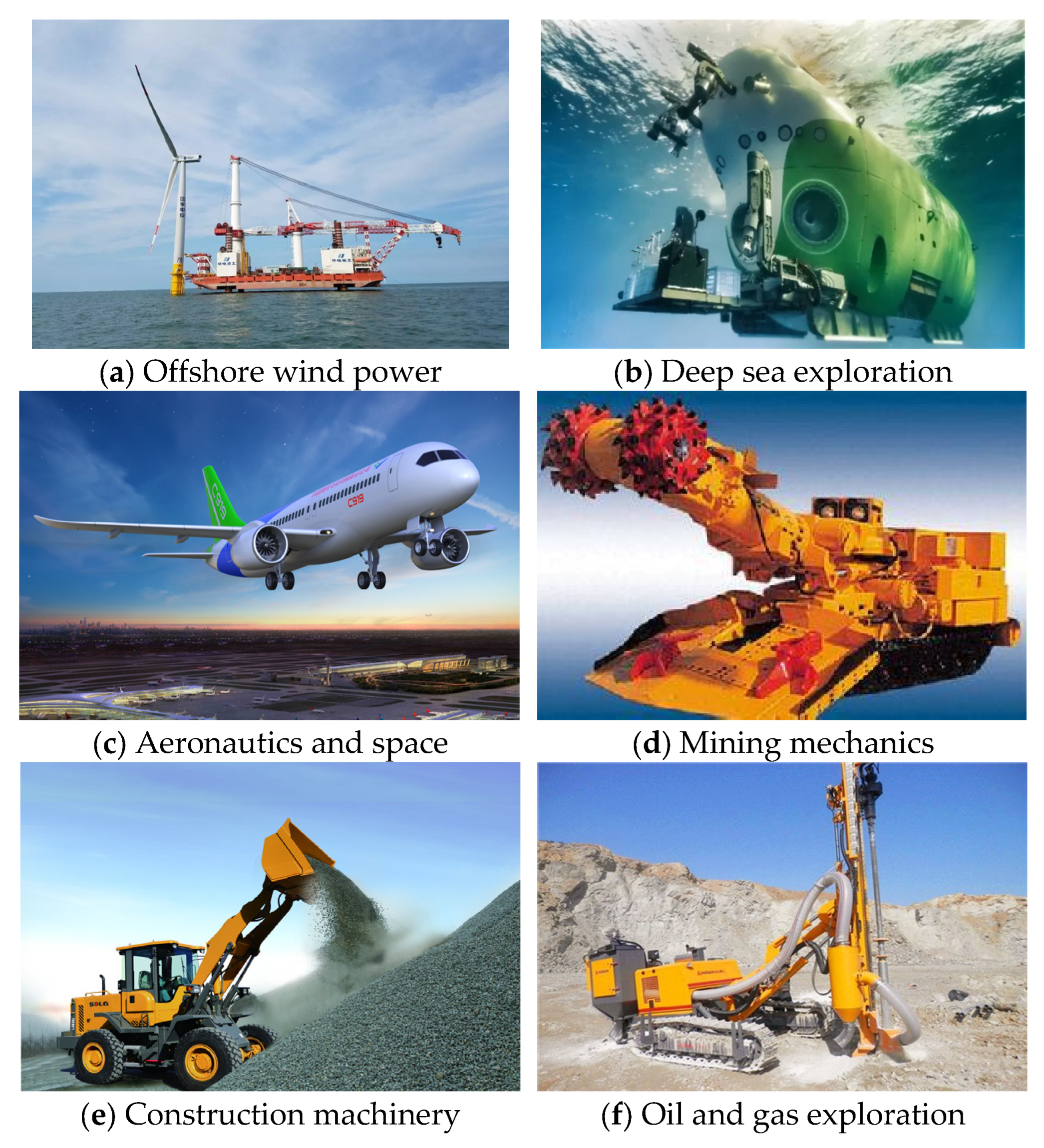
Hydraulic transmission has the advantages of high power density, fast response speed, and high load resistance stiffness [1], which is widely used in marine equipment, aerospace equipment, mining machinery, construction machinery, and other mechanical equipment (Figure 1) [2,3,4]. Among them, the working environment of marine engineering machinery and equipment is very complex and harsh, and it has the high requirements for the safety, stability, and reliability of its hydraulic transmission system [5,6,7]. As one of the commonly used “power hearts” of hydraulic transmission systems, axial piston pumps have a very wide range of applications in the fields of hydraulic transmission and intelligent control due to their small moment of inertia, compact structure, high rotational speed, easy variables, and other characteristics [8,9]. It plays a vital role in ensuring the stability and reliability of the hydraulic transmission system. 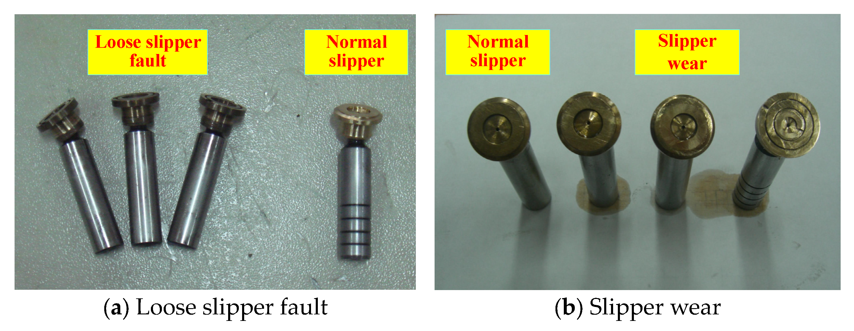However, the structure of a hydraulic axial piston pump is complex, and it often faces harsh working conditions such as high pressure and variable load [10,11]. The key components such as slipper, swash plate, and central spring are prone to wear failure. The failure will lead to the unstable operation of the hydraulic system, abnormal operation of the equipment, economic losses, and even endanger personal safety. Therefore, in order to ensure the safety and reliability of the whole machine and reduce the incidence of disaster accidents, it is very important to achieve an efficient, accurate, and intelligent diagnosis of typical faults of hydraulic axial piston pumps.

In 2006, Hinton first proposed the theory of deep learning (DL) in science. Since then and in recent years, the fault diagnosis of mechanical equipment has always attracted the attention of domestic and foreign scholars [12]. With the development of science and technology, DL has been widely used and achieved great success in computer vision, natural language processing, image processing, and other fields [13,14]. At the same time, the emergence of DL also brings new ideas and methods for intelligent fault diagnosis of mechanical equipment such as hydraulic axial piston pumps.

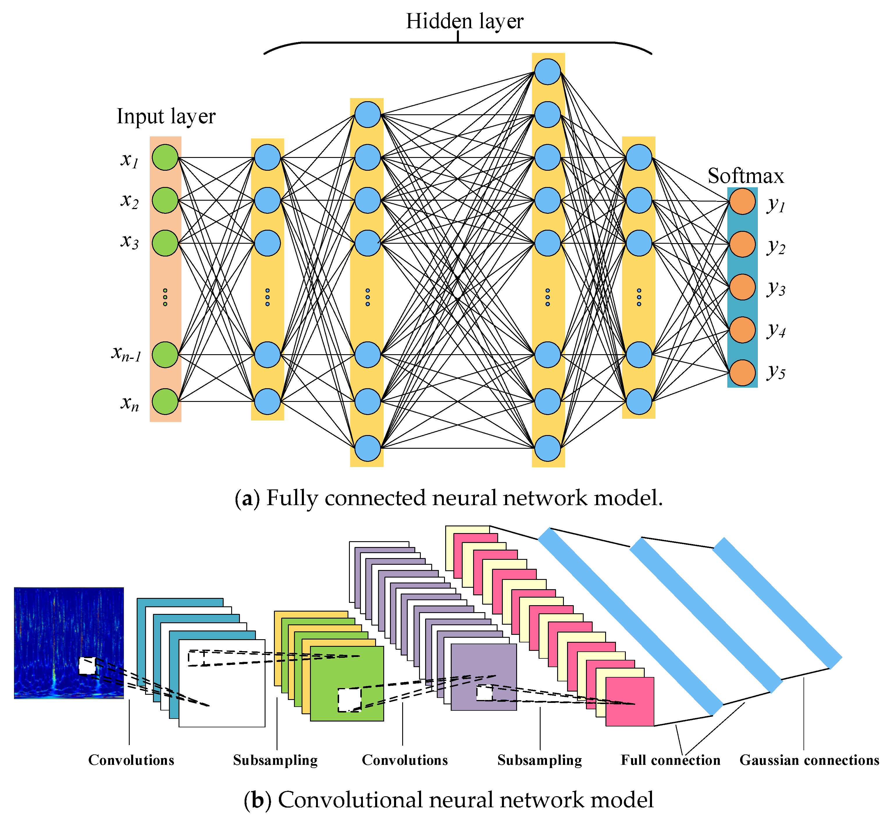
The intelligent fault diagnosis method of mechanical equipment based on the DL theory is typically represented by convolutional neural networks (CNNs). The commonly used CNN models include LeNet-5, AlexNet, VGG, and GoogLeNet. Owing to the powerful self-learning ability and feature extraction ability of the CNN, it has been applied in the field of fault diagnosis. To solve the problem of low diagnostic accuracy caused by insufficient samples, Zhao et al. used stochastic wavelet expansion for data enhancement and generated synthetic samples as training sets to train a one-dimensional CNN with two-layer convolution. The fault diagnosis of aero hydraulic pumps was achieved with small samples. The complex and changeable working conditions made the failure mechanism of mechanical equipment unclear, and it is difficult to use feature matching for fault diagnosis [15]. By using a CNN model structure with five hidden layers, Wang et al. proposed a CNN method for fault classification based on the minimum entropy deconvolution. Compared with the traditional CNN method, this method can better complete the multi-fault classification of axial piston pumps [16]. By combing the ResNet model, He et al. proposed a multi-signal adversarial fusion model based on transfer learning. The method solved the problem of fault diagnosis of hydraulic axial piston pumps under the condition of uneven data distribution. The average diagnosis accuracy reached more than 98.5% [17]. By using spectral denoising and the improved LeNet-5 model, Chao et al. processed one-dimensional vibration data through the short-time Fourier transform to complete the fault identification of high-speed axial piston pumps. The method significantly improved the CNN model in the noise environment. In order to further improve the fault diagnosis performance of axial piston pumps, a decision-level multi-sensor fusion diagnosis method was proposed. The vibration data of three channels were sent to three identical LeNet-5 models to generate preliminary classification results. Then, the results were fused to obtain the final prediction results [18]. The classification accuracy was increased by about 2%, 4%, and 5% after fusion [19]. To achieve the deep mining of features, Tang et al. constructed an adaptive LeNet-5-Bayesian optimization model based on the Gaussian process, and carried out the fault diagnosis of an axial piston pump driven by the vibration signal. Compared with the traditional LeNet-5, the accuracy was increased by 2.92%, and the typical fault states of an axial piston pump were effectively identified [20]. The above models were applied to the pressure signal analysis to achieve the fault diagnosis of axial piston pumps. The average accuracy of fault diagnosis reached 99.51%, which was 5.45% higher than the traditional LeNet-5 model [21]. Due to the dependence on a large number of signal processing techniques and expert diagnosis experience as well as the time-consuming limitations of data pre-processing of traditional mechanical fault diagnosis, Zhu et al. constructed a particle swarm optimization (PSO)-Improved-CNN diagnostic model to classify and identify the typical state data of hydraulic piston pumps and obtained a high diagnosis accuracy of 99.06% [22]. To solve the uncertainty of manual parameter adjustment, they continued the research and identified the fault of an axial piston pump based on acoustic signals compared with the classical CNN models such as AlexNet, VGG11, VGG13, VGG16, and GoogLeNet; the results indicated that the method had stronger stability and higher diagnostic accuracy [23]. For other rotating machinery, Sinitsin et al. combined with hybrid input for rolling bearing diagnosis, a bearing fault diagnosis method is proposed based on the hybrid CNN–MLP model. The hybrid model is superior to CNN and MLP models in separation, and the detection accuracy of bearing fault can reach 99.6% [24]. Choudhary et al. used multi-input convolutional neural net-work (MI-CNN) technology to fuse the characteristics of vibration signals and acoustic signals, and proposed a vibration–acoustic fusion technology for the fault diagnosis of induction motors under different working conditions. The effectiveness of the method is verified by bearing and gearbox datasets. This method can accurately and efficiently achieve the fault diagnosis of the motor and can be applied to other rotating machinery [25]. Glowacz proposed a new feature extraction method named power of normalized image difference (PNID). The deep neural networks GoogLeNet, ResNet50, and EfficientNetB0 were used to analyze the thermal image of the fault axis of the brushless DC motor, and a high-precision fault diagnosis was achieved [26]. As compound faults are difficult to accurately identify, Dibaj et al. used only a single fault dataset to train the CNN. When the obtained CNN output probability meets a set of probabilities, the untrained compound fault state is alarmed. The performance of the fine-tuning VMD and the proposed hybrid method was evaluated by decomposing the simulated vibration signal and analyzing the composite fault scenario of the gearbox system. The experimental results show that this method has high accuracy in compound fault diagnosis, small fault feature extraction, and serious fault classification [27].

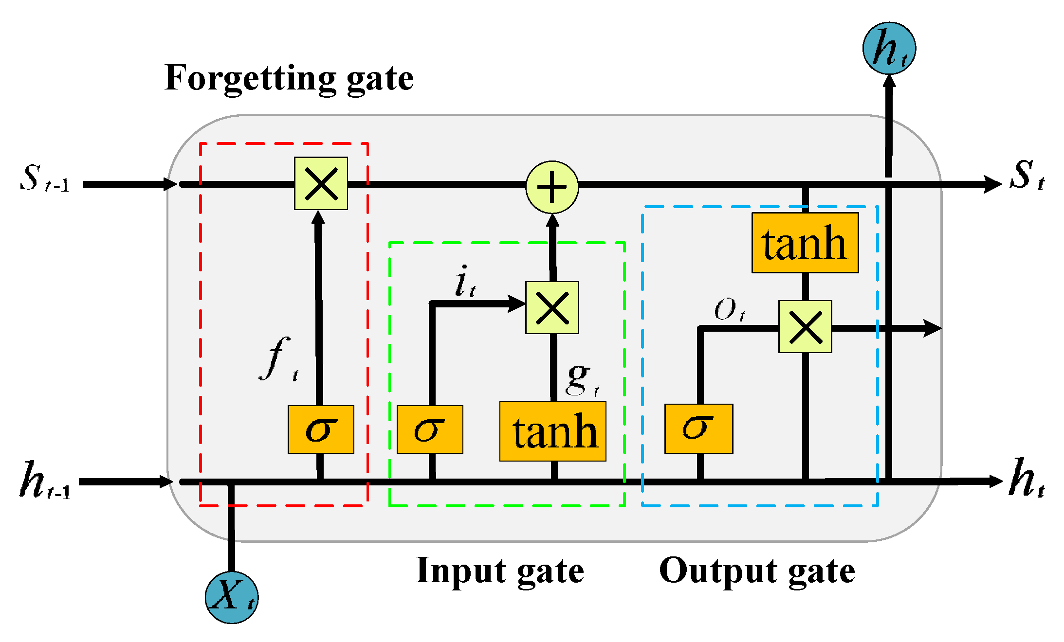
A recurrent neural network (RNN) is also the main model of deep neural networks. Long short-term memory (LSTM) is a variant of an RNN, which solves the problem of training difficulty from gradient disappearance and gradient explosion in ordinary recurrent neural networks. It is more suitable for processing time series information. LSTM has successful applications in speech recognition, text recognition, and is also used in the field of fault diagnosis of mechanical equipment [28,29]. To improve the operational reliability of the wind turbine gearbox, Zhu et al. proposed an evaluation framework of DL-based multi-indicator operating conditions to predict the real-time operation state of wind turbines based on LSTM networks by analyzing the operating condition monitoring data of wind turbines. The method effectively detected the potential faults of wind turbines [30]. In view of the inconsistent distribution of fault monitoring data among wind turbines, a prediction method combined with LSTM, fuzzy synthesis, and feature transfer learning was proposed to sensitively detect potential faults of wind turbines, which could effectively predict the operating state of the wind turbine [31]. By using 1D-CNN for feature extraction and combining it with the temporal correlation between LSTM learning features, Sun et al. proposed a fault diagnosis method based on 1DCNN-LSTM and LeNet-5 to achieve the end-to-end intelligent fault diagnosis of bearings [32]. The average fault recognition accuracy rate reached more than 99%. By decomposing the vibration signal of the reciprocating pump, Bie et al. proposed an improved deep neural network based on the adaptive noise empirical mode decomposition method [33]. They established a classification model based on the LSTM deep network to accurately identify the failure mode. Zhao et al. combined CNN and LSTM networks to achieve multi-fault classification of the main pump of a converter station, with the accuracy rate of 98.7% [34]. By using LSTM, Khan et al. evaluated the operating state of industrial mud pumps to achieve the prediction of the remaining life [35]. At present, although the application of LSTM in the field of mechanical equipment fault diagnosis is gradually expanding, there are relatively few studies on fault diagnosis of axial piston pumps based on RNNs.

The fault data of the axial piston pump have evident temporality. The RNN model can effectively and accurately process this type of data, while it has no feature extraction capability and generally takes time domain or frequency domain signals as part of the preprocessing. These preprocessing methods do not have high feature extraction efficiency as does a CNN, and the relevant parameters also need to be manually adjusted under multiple working conditions. CNNs and RNNs are the two most common deep learning networks. They are widely used in fault diagnosis of hydraulic axial piston pumps, but there are still some challenges and problems in the current research.

(1) Most of the research on deep learning models focuses on the intelligent fault diagnosis of bearings, gearboxes, and motors, and is still relatively rare on hydraulic axial piston pumps. The structure and working mechanism of this kind of pump are complex. The concealment and coupling of its faults make it more valuable and challenging for fault diagnosis and condition monitoring.

(2) The traditional intelligent diagnosis method performs time-consuming preprocessing on the original signal. In addition, the understanding of equipment failure mechanism and data preprocessing technology is stricter.

(3) CNN does not have memory ability, and the calculation time is too long; LSTM cannot effectively address high-dimensional data, and there will be a long-term dependence problem when the sample sequence is too long. It is difficult to identify when addressing faults with similar features.

Therefore, the main contributions of this work are as follows:

(1) Aiming at the special structure and mechanism of a hydraulic axial piston pump, the intelligent fault diagnosis of a hydraulic axial piston pump is explored. Non-destructive condition monitoring is achieved by using the characterization information of pump body as data source. It makes full use of the characteristics of the original sensor information in the time domain and frequency domain, eliminating the complex and time-consuming signal preprocessing steps.

(2) Different working conditions are set up, and different wear degrees of the same fault type are included in the analysis. The performance of the proposed method is discussed from different perspectives. Using the feature extraction ability of a CNN for high-dimensional information and the high-precision recognition ability under supervised learning, the time–frequency feature self-learning and classification of the hydraulic axial piston pump are achieved.

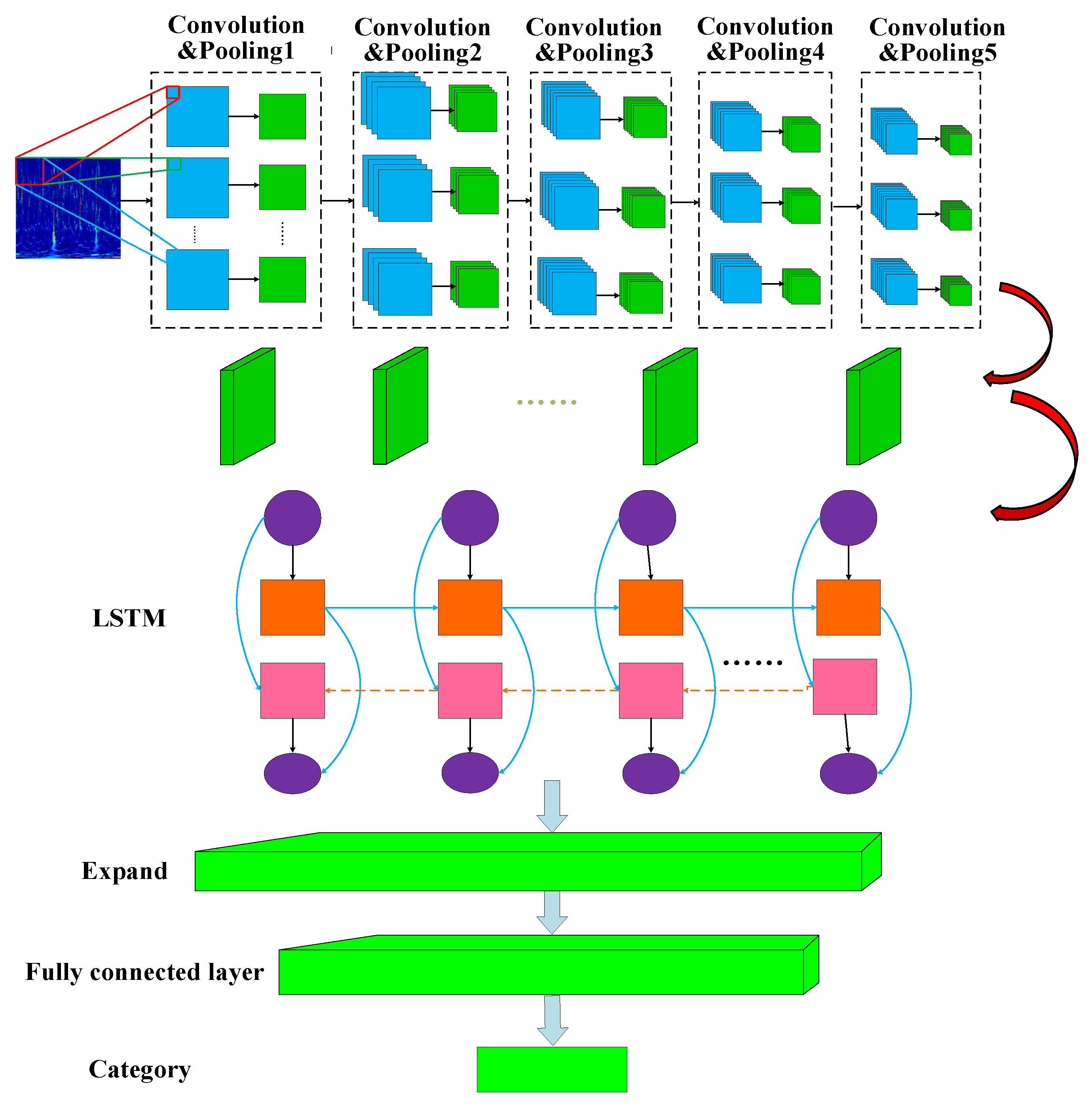
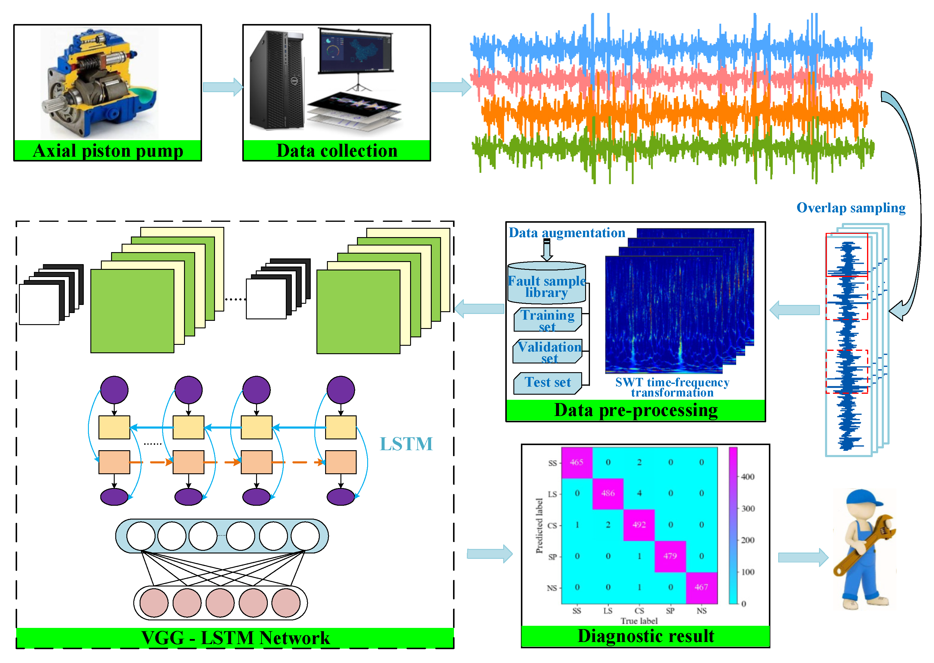
(3) A fault diagnosis model combining efficient feature extraction of VGG network and time series information learning of the LSTM model is proposed. Combined with the SWT time–frequency feature extraction method, intelligent fault diagnosis of a hydraulic axial piston pump is carried out, which enhances feature extraction ability, shortens calculation time, and improves fault diagnosis accuracy and efficiency.

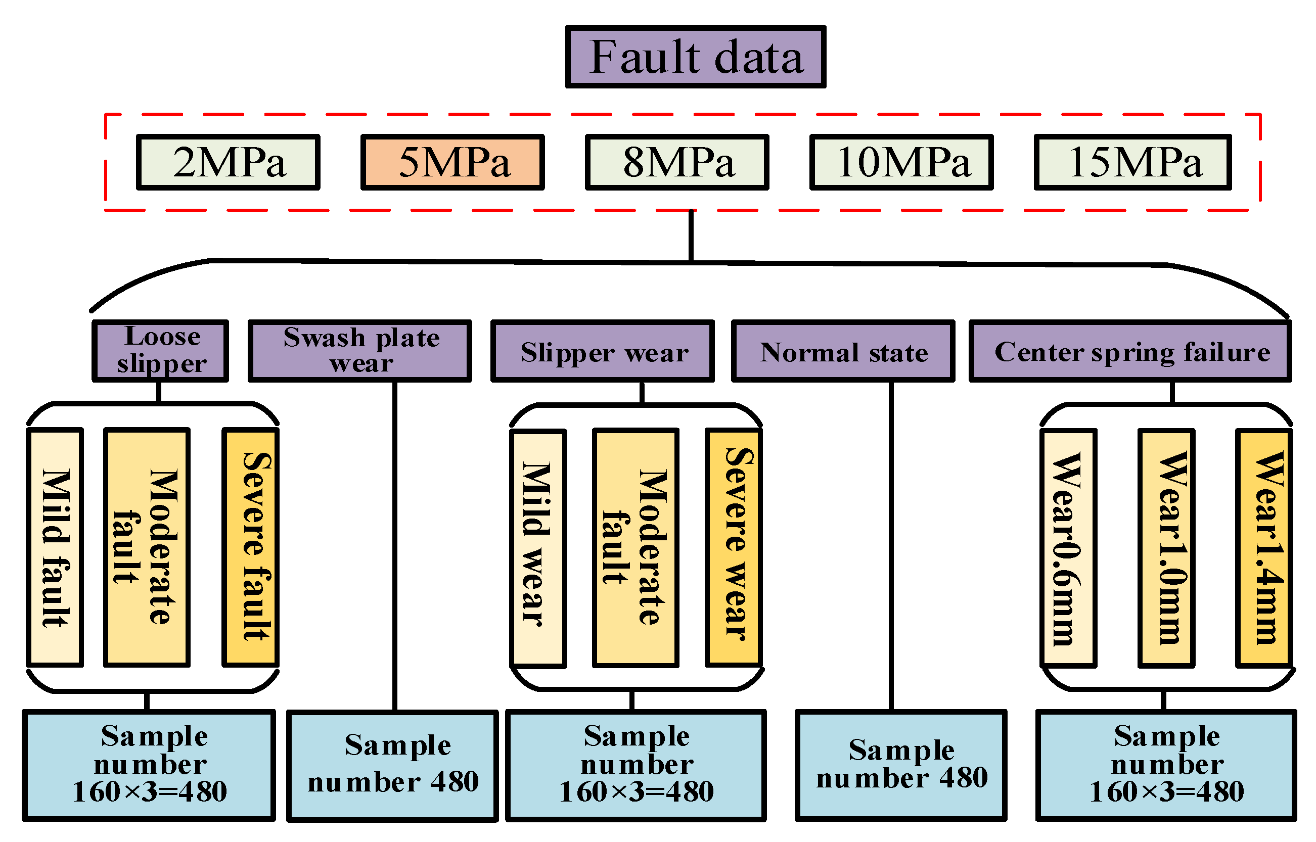
The rest of the main structure is as follows. In Section 1, the basic principle of the SWT, CNN, and LSTM algorithm is summarized. In Section 2, the implementation process of the intelligent fault diagnosis method based on the improved VGG–LSTM fusion model is introduced. Section 3 analyzes the collection of experimental data and the construction process of fault samples in detail. Section 4 conducts comparison experiments and analyzes the main results. Finally, conclusions are summarized and the future research is prospected in Section 5.

2. Basic Theory

2.1. Synchrosqueezing Wavelet Transform

SWT is a time–frequency redistribution method proposed by Daubechies et al. by combining synchronous compression technology with the continuous wavelet transform (CWT) [36,37]. One principle applied in this method is that the scale change cannot affect the phase of the signal after wavelet transform. Then, the scales are added at the same frequency. Additionally, the coefficients around the same frequency are compressed to this frequency by combining the synchronous compression technology. According to the size of each element mode in the time–scale plane, the energy of the time–scale plane is redistributed. Finally, the time–scale plane is transformed into the time–frequency plane through a special mapping relationship, and the spectrum with concentrated coefficients is obtained to improve the time–frequency resolution of the signal. The higher time–frequency concentration and the finer time–frequency line are achieved. Compared with the conventional wavelet transform, SWT has a higher time–frequency resolution.

Let us suppose $\psi$ is a square-integrable function, a family of functions is defined as follows:

$${\psi }_{\alpha ,\tau }\left(t\right)={\left|\alpha \right|}^{-1/2}\psi \left(\frac{t-\tau }{\alpha }\right)$$

(1)

where $\alpha$ is the scaling factor, $\alpha \in R$ and $\alpha \ne 0$, $\tau$ is the translation factor, and ${\psi }_{\alpha ,\tau }\left(t\right)$ is the continuous wavelet. Let the input signal $S\left(t\right)\in L^2\left(R\right)$; then, its CWT expression is

$$CW{T}_S\left(\alpha ,\tau \right)=〈S\left(t\right),{\psi }_{\alpha ,\tau }〉={\left|\alpha \right|}^{-1/2}{\displaystyle {\int }_{-\infty }^{+\infty }S\left(t\right)\overline{\psi \left(\frac{t-\tau }{\alpha }\right)}dt}$$

(2)

where $\overline{\psi \left(\frac{t-\tau }{\alpha }\right)}$ is the complex conjugate of $\psi \left(t\right)$, $〈S\left(t\right),{\psi }_{\alpha ,\tau }〉$ denotes the inner product of $S\left(t\right)$, and ${\psi }_{\alpha ,\tau }$.

According to Plancherel’s theorem, rewriting $CW{T}_S\left(\alpha ,\tau \right)$ as CWT of signal $S\left(t\right)$ in the frequency domain:

$$CW{T}_S\left(\alpha ,\tau \right)=\frac{1}{2\pi }{\left|\alpha \right|}^{1/2}{\displaystyle {\int }_{}^{}\stackrel{\wedge }{S}\left(\xi \right)\overline{\stackrel{\wedge }{\phi }\left(\alpha \xi \right)}{{\displaystyle e}}^{\mathrm{i}b\xi }d\xi }$$

(3)

where $\xi$ is the angular frequency and $\stackrel{\wedge }{S}\left(\xi \right)$ is the Fourier transform of the signal $S\left(t\right)$. When the wavelet transform coefficient at any point $(\alpha ,\tau )$ is not equal to zero, the instantaneous-frequency $CW{T}_S\left(\alpha ,\tau \right)$ of the signal $S\left(t\right)$ is

$${\omega }_S(\alpha ,\tau )=-\mathrm{i}{(CW{T}_S(\alpha ,\tau ))}^{-1}\frac{\partial }{\partial b}CW{T}_S(\alpha ,\tau )$$

(4)

Then, a synchronous compression transformation is performed to establish the mapping from the starting point $(\tau ,\alpha )$ to $(\tau ,{\omega }_S(\alpha ,\tau ))$, $CW{T}_S\left(\alpha ,\tau \right)$ et al. is transformed from the time–scale plane to the time–frequency scale plane to obtain the new time–frequency spectral map.

In practical applications, it is necessary to first discretize the frequency variable $\omega$, the scale variable $\alpha$, and the displacement variable $\tau$. When the frequency $\omega$ and the scale $\alpha$ are discrete variables, and ${\alpha }_k-{\alpha }_{k-1}={({\Delta }\alpha )}_k$ is satisfied at the point ${\alpha }_k$, $CW{T}_S\left(\alpha ,\tau \right)$ can be obtained. Its corresponding synchronous compression transform $T_S\left(\alpha ,\tau \right)$ can likewise be accurately calculated only when the continuous interval $[\omega -\raisebox{1ex}{$1$}\!\left/ \!\raisebox{-1ex}{$2$}\right.{\Delta }\omega ,\omega +\raisebox{1ex}{$1$}\!\left/ \!\raisebox{-1ex}{$2$}\right.{\Delta }\omega ]$ satisfies ${\omega }_{\mathcal{\ell }}-{\omega }_{\mathcal{\ell }-1}={\Delta }\omega$. Finally, the expression of the simultaneous compressive wavelet transform is obtained by combining different conditions:

$$T_S\left({{\displaystyle \omega }}_{\mathcal{\ell }},\tau \right)={\Delta }{{\displaystyle \omega }}^{-1}{\displaystyle \sum _{{\alpha }_k:\left|\omega ({\alpha }_k,\tau )-{{\displaystyle \omega }}_{\mathcal{\ell }}\right|}CW{T}_S\left({\alpha }_k,\tau \right)}{\alpha }_k{}^{-\frac{3}{2}}{({\Delta }\alpha )}_k$$

(5)

2.2. CNN

The CNN is relatively mature in the development of DL models, which are widely used in image recognition and speech analysis [38,39]. The CNN can be considered as a multilayer fully connected neural network based on the addition of convolutional layers, pooling layers, etc. The network is formed by stacking each processing layer, as shown in Figure 2. The commonly used classical CNN models are LeNet-5, AlexNet, VGGNet et al. [40,41,42]. As a feed-forward neural network, it contains two parts: feature self-learning and classification [43]. Feature self-learning is usually performed in the convolutional and pooling layers. The classification task is mainly performed by the fully connected layer.

The convolutional layer is the core of the CNN. A convolutional layer can contain different feature information extracted from multiple convolutional kernels [44]. The more layers, the richer the data extraction, the more evident the features. Let us suppose the input feature map of the vibration signal to be y; then, the convolution layer operation formula can be described as follows:

$$y_j^{l+1}=f\left({\displaystyle \sum _{i=1}^M\left(x_i^l\otimes k_{ij}^l\right)}+b_j^l\right)$$

(6)

where $y_j^{l+1}$ denotes the input of the j-th neuron in layer l + 1; f is the activation function; and M denotes the number of feature maps. $x_i^l$ denotes the output of the i-th neuron in layer l. $\otimes$ denotes the convolution operation. $k_{ij}^l$ denotes the convolution kernel of the i-th neuron in layer l with the j-th neuron in layer l + 1. b denotes the bias. The calculation process of the convolution layer is displayed in Figure 3. The original feature map is of size 6 × 6, and the output feature map is 3 × 3 after the convolution calculation.

As a down-sampling structure acting between successive convolutional layers, a pooling layer generally includes a maximum pooling layer, an average pooling layer, and a random pooling layer. The maximum pooling layer and the average pooling layer extract the maximum value and average value of the pooling window as the output result. Then, sliding the window continuously reduces the size of the input data so as to reduce the redundant information. Among them, the maximum pooling is most used in the convolutional neural network. The maximum pooling is presented in Equation (7) and given schematically in Figure 4.

$$P_j^{l+1}(i)=ma{x}_{(i-1)W+1\le t\le iW}\left\{a_j^l(t)\right\}$$

(7)

In this research, the cross-entropy loss function is utilized. After the error value of back propagation is calculated by the neural network via derivation, the value of the weight matrix is corrected to update the weight. The expression of the weight update formula is

$$W^{+}=W-\eta \frac{\partial L\mathrm{oss}}{\partial W}$$

(8)

where $W$ represents the weight, $\eta$ is the learning rate, and $Loss$ represents the loss function.

The fully connected layer integrates the extracted features from the previous layers, maps the high-dimensional feature map into a vector of fixed dimensions, and finally completes the pattern recognition in the classifier.

2.3. LSTM

As a variant of the RNN, the LSTM is a temporal recurrent neural network to alleviate the gradient problem of the RNN during training [45,46]. By introducing the gate function, it can tap into the relatively long intervals and delays in time series [47]. With a certain ability to learn to long-term dependent information, the LSTM effectively overcomes the gradient disappearance or explosion problem, which is applied in major fields, such as language translation, audio analysis, remaining life prediction, etc. [48,49,50,51]. The LSTM controls the information flow through three gates: input gate, forget gate, and output gate [52]. Its basic network structure is revealed in Figure 5.

The input $x_t$, the state memory unit $S_{t-1}$, and the intermediate output $h_{t-1}$ in the forgetting gate determine the forgetting part of the state memory unit together. The $x_t$ in the input gate is jointly determined to retain the vector in the state memory cell through respective changes of sigmoid and tanh function. The intermediate output $h_t$ is determined by the updated $S_t$ and the output $o_t$ together. The calculation formula is as follows:

$$f_t=\sigma \left(W_{fx}{x}_t+W_{fh}{h}_{t-1}+b_f\right)$$

(9)

$$i_t=\sigma \left(W_{ix}{x}_t+W_{ih}{h}_{t-1}+b_i\right)$$

(10)

$$g_t=\varphi \left(W_{gx}{x}_t+W_{gh}{h}_{t-1}+b_g\right)$$

(11)

$$o_t=\sigma \left(W_{ox}{x}_t+W_{oh}{h}_{t-1}+b_o\right)$$

(12)

$$S_t=g_t\Theta i_t+S_{t-1}\Theta f_t$$

(13)

$$h_t=\varphi \left(S_t\right)\Theta o_t$$

(14)

where $f_t$, $i_t$, $g_t$, $o_t$, $h_t$, and $S_t$ are the states of the oblivion gate, input gate, input node, output gate, intermediate output, and state unit. $W_{fx}$, $W_{fh}$, $W_{ix}$, $W_{ih}$, $W_{gx}$, $W_{gh}$, $W_{ox}$, and $W_{oh}$ are the matrix weights of the corresponding gates multiplied by the input $x_t$ and intermediate output $h_{t-1}$. $b_f$, $b_i$, $b_g$, and $b_o$ are the bias terms of the corresponding gates. $\Theta$ denotes the bitwise multiplication of the elements in the vector. $\sigma$ denotes the change in sigmoid function. $\varphi$ denotes the change in tanh function.

In the LSTM, there are three sources of information flow, namely input $x_t$ at the current moment, hidden state $h_{t-1}$ at the previous moment, and neuron state $S_{t-1}$ at the previous moment. The fundamental information flow is only the current input $x_t$ and the previous hidden state $h_{t-1}$, which controls the data update.

$$new=\varphi (W_{xs}{x}_t+W_{hs}{h}_{t-1}+b_s)$$

(15)

In this research, dropout technology is adopted into the LSTM layer, setting p = 0.5. In the process of model training, some neurons are randomly deactivated, and the corresponding parameters will not be calculated. In this way, the model can randomly ignore some details of the input data. The over-fitting problem can thereby be prevented to identify the target from the overall information.

3. Intelligent Fault Diagnosis Model

Combining the characteristics of the vibration signal of the hydraulic axial piston pump and the respective advantages of the CNN and LSTM in deep learning, this paper constructs an intelligent fault diagnosis model based on VGG–LSTM, which integrates depth feature mining with fault pattern recognition. By introducing the LSTM, the method has a certain feature memory capability, which achieves an efficient and accurate intelligent fault diagnosis of hydraulic axial piston pumps.

3.1. Model Construction

The VGG–LSTM model is a new network fusion method proposed in this paper. Combining the respective advantages of VGG11 and LSTM, an LSTM network is added after the last pooling layer of the VGG11 network for training. Finally, the feature graph is expanded into a 1D vector input into the full connection layer, and the mapping between feature vector and fault category is established. The specific network structure parameters are shown in

Table 1. Structure parameters of VGG–LSTM network.

Network Layer	Output Dimension	Parameter Setting
Conv1	224 × 224	$\left[\begin{array}{c}3 \times 3, 64\\ 3 \times 3, 64\end{array}\right]$
Pool1	112 × 112	2 × 2 maxpooling, stride = 2
Conv2	112 × 112	$\left[\begin{array}{c}3 \times 3, 128\\ 3 \times 3, 128\end{array}\right]$
Pool2	56 × 56	2 × 2 maxpooling, stride = 2
Conv3	56 × 56	$\left[\begin{array}{c}3 \times 3, 256\\ 3 \times 3, 256\end{array}\right]$ × 2
Pool3	28 × 28	2 × 2 maxpooling, stride = 2
Conv4	28 × 28	$\left[\begin{array}{c}3 \times 3, 512\\ 3 \times 3, 512\end{array}\right]$ × 2
Pool4	14 × 14	2 × 2 maxpooling, stride = 2
Conv5	14 × 14	$\left[\begin{array}{c}3 \times 3, 512\\ 3 \times 3, 512\end{array}\right]$ × 2
Pool5	7 × 7	2 × 2 maxpooling, stride = 2
LSTM	49 × 1	-
Fc	1 × 1	64
-	1 × 1	Output, 5, Softmax

, and the model structure is presented in Figure 6. The model has eight convolutional layers, five maximum pooling layers, one LSTM network layer and one fully connected layer. The convolution layer uses a 3 × 3 convolutional kernel to extract features and activates the output by the ReLU function. The pooling layer uses a 2 × 2 convolutional kernel to reduce the dimensionality of the input data. The ratio of the dropout layer is set to 0.5. After several stacked convolutional pooling operations, the size of the output feature map changes from (224, 224, 3) to (7, 7, 512). The size of the output feature map is reconstructed to (49, 512) by the Reshape method, and further input to the LSTM network to extract the corresponding temporal information. After analyzing the temporal features, the images are sorted using the fully connected layer to determine their affiliation classes.

3.2. Diagnostic Process

Figure 7 shows the whole process of fault diagnosis of a hydraulic axial piston pump based on the SWT time–frequency analysis and the VGG–LSTM fusion model.

The specific diagnostic steps are as follows:

Step 1: The original vibration signals of the piston pump in different states are collected by the sensors mounted on the axial piston pump.

Step 2: The collected original signals are resampled, and the training samples are added to improve the generalization ability of the network model.

Step 3: The processed time domain data are converted into two-dimensional time–frequency diagrams by SWT. The images are data-enhanced by random rotation, flip, scale transformation, and translation. Finally, the signals are transformed into a 224 × 224 × 3 RGB time–frequency image dataset.

Step 4: Based on Python programming, the two-dimensional time–frequency diagrams are divided into training set, validation set, and test set according to a certain number of proportions. The corresponding labels are added to make the number of samples in each fault state reach a balance. Finally, the fault sample library is constructed.

Step 5: The training set is fed into the constructed fusion model for learning and training while the parameters of manual tuning are performed. The optimal hyperparameters’ combination and the final model for testing are identified.

Step 6: The determined optimal diagnostic model is used to identify the test set, and the final state identification results of hydraulic piston pump are obtained.

Step 7: The standard CNN model and the standard LSTM model with different layers are built based on the Pytorch framework. The stability and robustness of the model are verified by comprehensive comparison with the constructed model. The standard CNN models include LeNet-5, AlexNet, and VGG11, and the standard LSTM models comprise one, two, and three layers.

4. Experimental Data Collection and Sample Construction

4.1. Status Signal Acquisition

The test bench of the hydraulic axial piston pump is built, as shown in Figure 8. The model of the axial piston pump is MCY14-1B, the theoretical displacement is 10 mL/r, the nominal pressure is 31.5 MPa, and the drive motor is Y132M-4. The rated speed is 1470 r/min. A piezoelectric accelerometer is employed for vibration signal acquisition, whose type is YD72-D, and its frequency range is 1~18 kHz. The vibration accelerometer is installed in the end cover of the pump shell by direct paste. The operating pressure of the piston pump is set at 2 MPa, 5 MPa, 8 MPa, 10 MPa, and 15 MPa. Under each operating pressure, the acceleration sensor is used to collect the vibration signals of five typical states of the piston pump. The five states include normal state, swash plate wear, loose slipper, sliding slipper wear, and center spring failure. The four typical faulty components are displayed in Figure 9. Figure 10 is the basic structure diagram of the hydraulic axial piston pump, which is a pump with fixed displacement. The pitch diameter of the arrangement of the pistons in the cylinder block is 43 mm and their number is 7. The angle of swash plate is 16°, the stroke of the pistons and springs are 13 mm and 5 mm, respectively. During the signal acquisition process, the piston pump operates at only one state. In addition to the normal operating state, the remaining four fault states of the piston pump are achieved by manually replacing the faulty components.

Figure 11 reveals the partial time domain waveforms of vibration signals under five different states when the working pressure of the hydraulic axial piston pump is 5 MPa. It can be seen from the diagrams that there is a difference in the time domain diagram of the vibration signal between the normal state and the fault states. When the piston pump fails, the amplitude changes, but the difference between the time domain diagrams can only assist in judging whether the piston pump fails, and the corresponding fault types cannot be directly identified.

4.2. SWT Time–frequency Feature Extraction

In order to obtain more relevant effective fault features, the vibration signals are converted to the time–frequency domain by using SWT for analysis, so as to better highlight the hidden information. After the SWT time–frequency characteristics are extracted, the data are enhanced using transforms. The time–frequency diagrams of the partial vibration signals of the five typical states of the hydraulic axial piston pump are presented in Figure 12. As can be seen in the figure, there are differences between the time–frequency diagrams of different state signals, and the performance characteristics of the time–frequency diagrams corresponding to different fault types are different. It is difficult to visually determine the type of fault corresponding to each time–frequency diagram. Therefore, a recognition model with self-learning is needed to identify the typical fault states of the piston pump.

4.3. Time–Frequency Feature Sample Library Construction

In order to investigate the effectiveness of the VGG–LSTM model in identifying different levels of fault in the hydraulic axial piston pump, in the experiment, three different degrees of faults including mild, moderate, and severe are set under the three states of loose slipper fault, slipper wear, and central spring failure. To ensure the balance of the sample data, the number of samples of each fault type should be kept consistent. When the operating pressure is 5 MPa, the composition of the sample library is described in Figure 13. The number of mild, moderate, and severe fault samples obtained by loose slipper, slipper wear, and central spring failure is 160, and the total number of samples is 480. In addition, the number of samples for different working pressures of swash plate wear and normal state signals is also 480. Since the vibration signals under five typical states are collected at operating pressures of 2 MPa, 5 MPa, 8 MPa, 10 MPa, and 15 MPa, the total number of vibration signal samples is 12,000.

The dataset of the constructed sample library is divided. The model learns the labeled training dataset to deepen the memory of each fault state information by supervised learning training. Finally, the model performs a predictive classification of the test dataset to achieve the identification of fault information. Therefore, it is necessary to divide the vibration signals time–frequency diagram database and add label operations before the model training. Samples are randomly selected under the same label and divided into training set, validation set, and test set to constitute the final dataset, of which 60% is the training set, 20% is the validation set, and 20% is the test set. The specific description is shown in

Table 2. Division of sample library.

Piston Pump Status		Sample Number		Label
	Training Set	Validation Set	Test Set
Normal state	1440	480	480	0
Swash plate wear	1440	480	480	1
Loose slipper fault	1440	480	480	2
Sliding slipper wear	1440	480	480	3
Center spring failure	1440	480	480	4

.

5. Results and Discussion

In order to verify the effectiveness of the proposed method, the performance of the traditional LSTM models, the classical CNN models (AlexNet, LeNet-5, VGG11) and the intelligent fault diagnosis model fused with SWT and VGG–LSTM are verified using the constructed sample library. The model parameters are set as follows: the number of images’ batch size is selected as 32, the number of iterative steps Epoch is preset as 70, the SGD algorithm is selected as the optimizer, Momentum is set as 0.9, cross-entropy is used as the loss function, and the learning rate is set as 0.001. The validation set verifies the model training effect and finetunes the model parameters based on the validation results. The deep learning framework is Pytorch (version 1.11.0+cu113), the development language is Python, and the hardware configuration of computer is Intel(R) Xeon(R) W-2235 CPU @ 3.80 GHz with 64 GB RAM.

5.1. Fault Diagnosis Based on Traditional LSTM Model

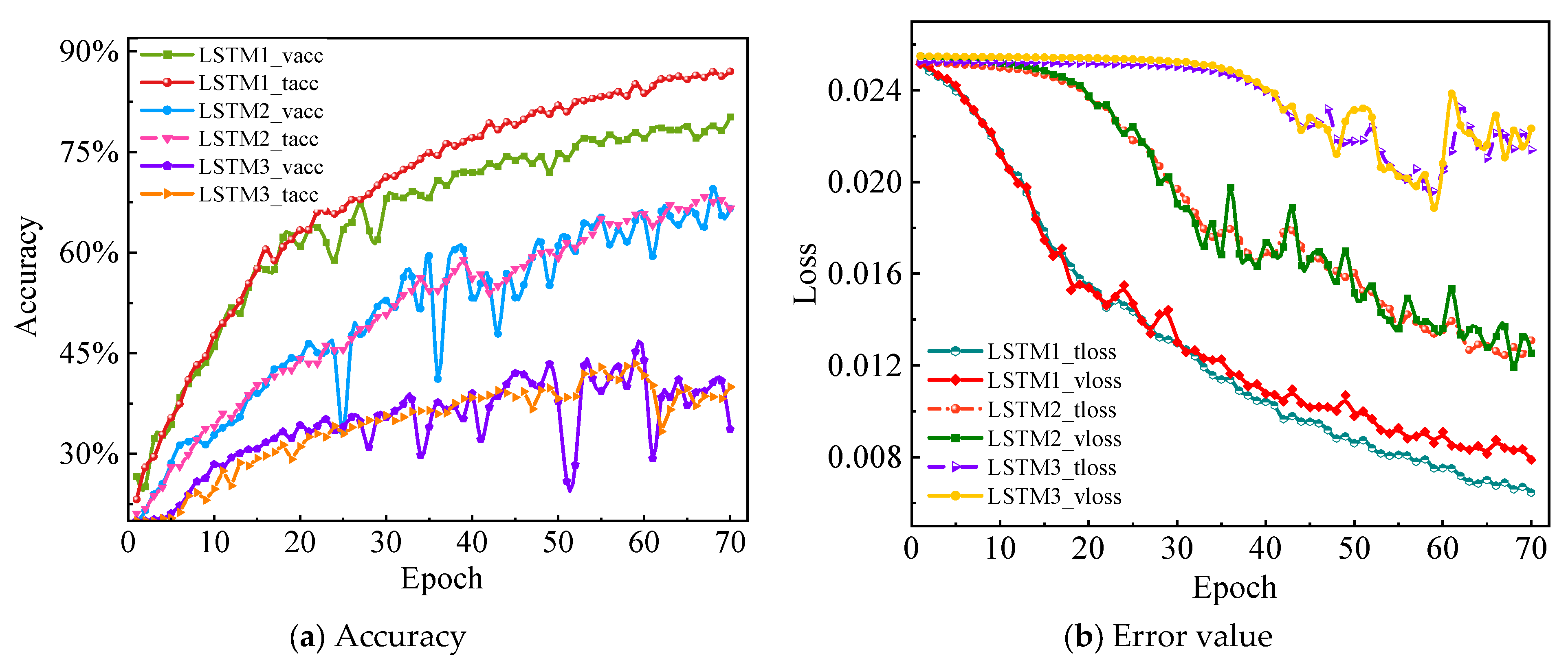
In order to test the performance of the model, the LSTM model (single-layer LSTM, double-layer LSTM, three-layer LSTM) is used for the fault diagnosis of the hydraulic axial piston pump on the same dataset. The diagnosis results are revealed in

Table 3. Results of different LSTM models.

Model	Accuracy of Training/%	Training Error Value	Training Time/s	Accuracy of Verification/%	Validation Error Value	Proof Time/s
Single-layer LSTM	85.14	0.00645	14.367	78.25	0.00788	5.373
Double-layer LSTM	65.32	0.01309	14.221	65.29	0.01253	5.691
Three-layer LSTM	39.42	0.02140	14.561	34.29	0.02233	5.627

. All model inputs are two-dimensional time–frequency diagrams, and the number of hidden nodes is set to 132 according to the complexity of the dataset. The comparison results of accuracy and error value of different models are shown in Figure 14. Combined with Table 3 and Figure 14, it can be seen that the single-layer LSTM model has better synthesis performance compared with the two-layer LSTM or three-layer LSTM. The accuracy curve is relatively stable in the training process, with a maximum accuracy of 85% for the training set and 78% for the validation set. The loss curve converges faster, and the training and validation error curves can drop to smaller values more rapidly and steadily.

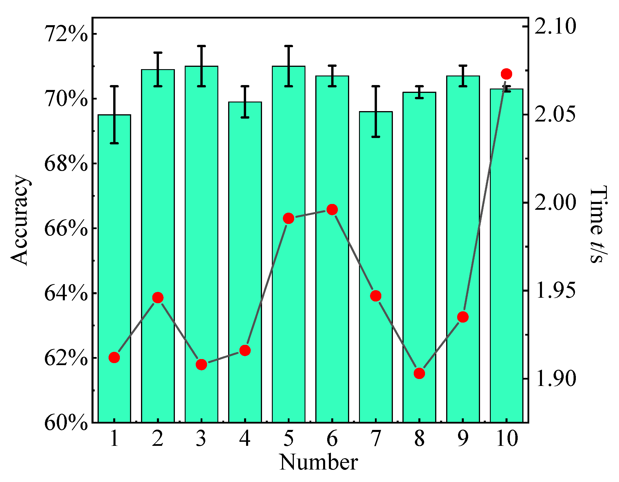
In order to verify the generalization of the single-layer LSTM model, the test set is used to test the performance of the trained model. Ten independent repeated tests are performed on the test set, and 20% of the samples are randomly selected from the dataset for each calculation. The test results are displayed in

Table 4. Repeated test accuracy and time of the single-layer LSTM mode.

Serial Number	1	2	3	4	5	6	7	8	9	10	Mean	Standard Deviation
Test accuracy/%	69.58	70.91	71.08	69.91	71	70.79	69.62	70.25	70.70	70.3	70.42	0.0050
Test time/s	1.912	1.946	1.908	1.916	1.991	1.996	1.947	1.903	1.935	2.073	1.912	0.0510

and Figure 15. According to Table 4 and Figure 15, the average accuracy of ten independent repeated tests is 70.42%, and the standard deviation is 0.005.

5.2. Fault Diagnosis Based on Classical CNN Models

In order to better select the optimal model for comparative testing, some classic CNN models (LeNet-5, AlexNet, VGG11) are utilized for the fault diagnosis of the same dataset. The training samples and verification samples are input into the established classic CNN models for training, and the test samples are used to test the performance of the models.

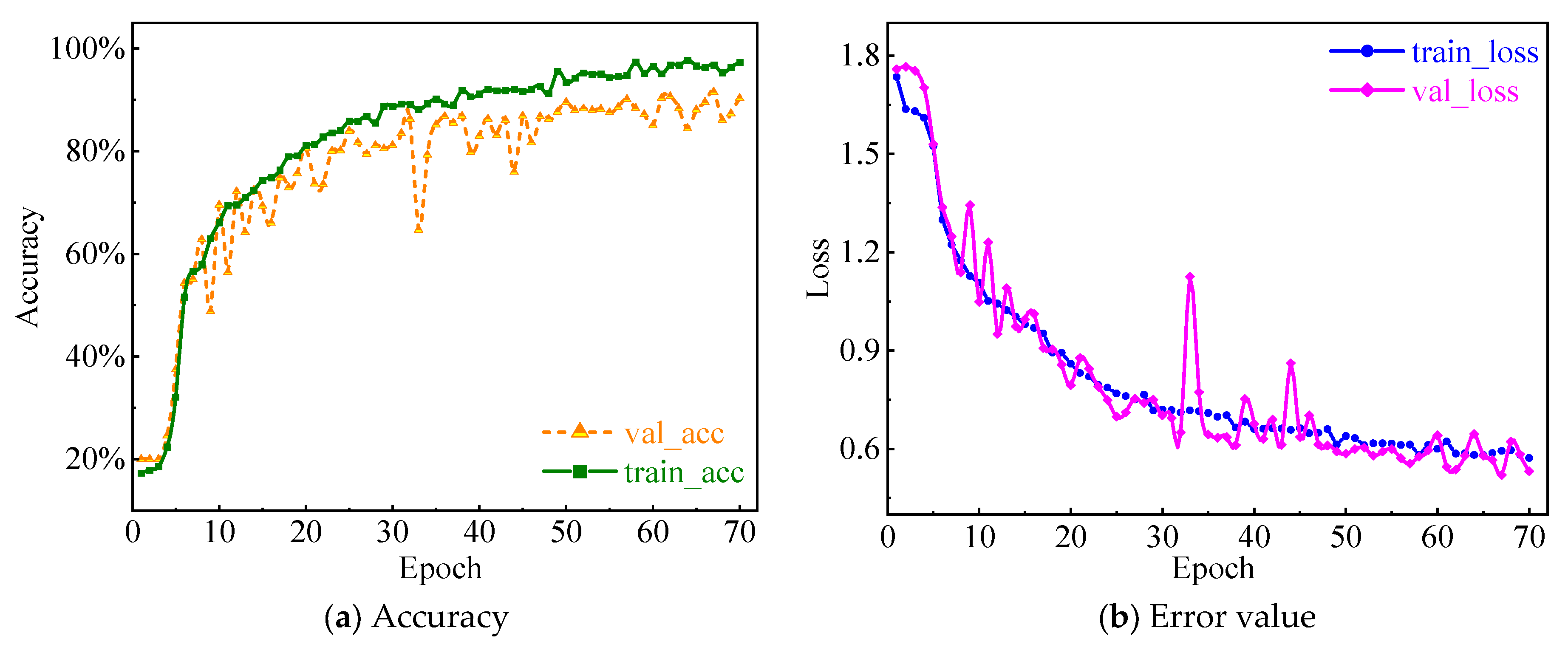
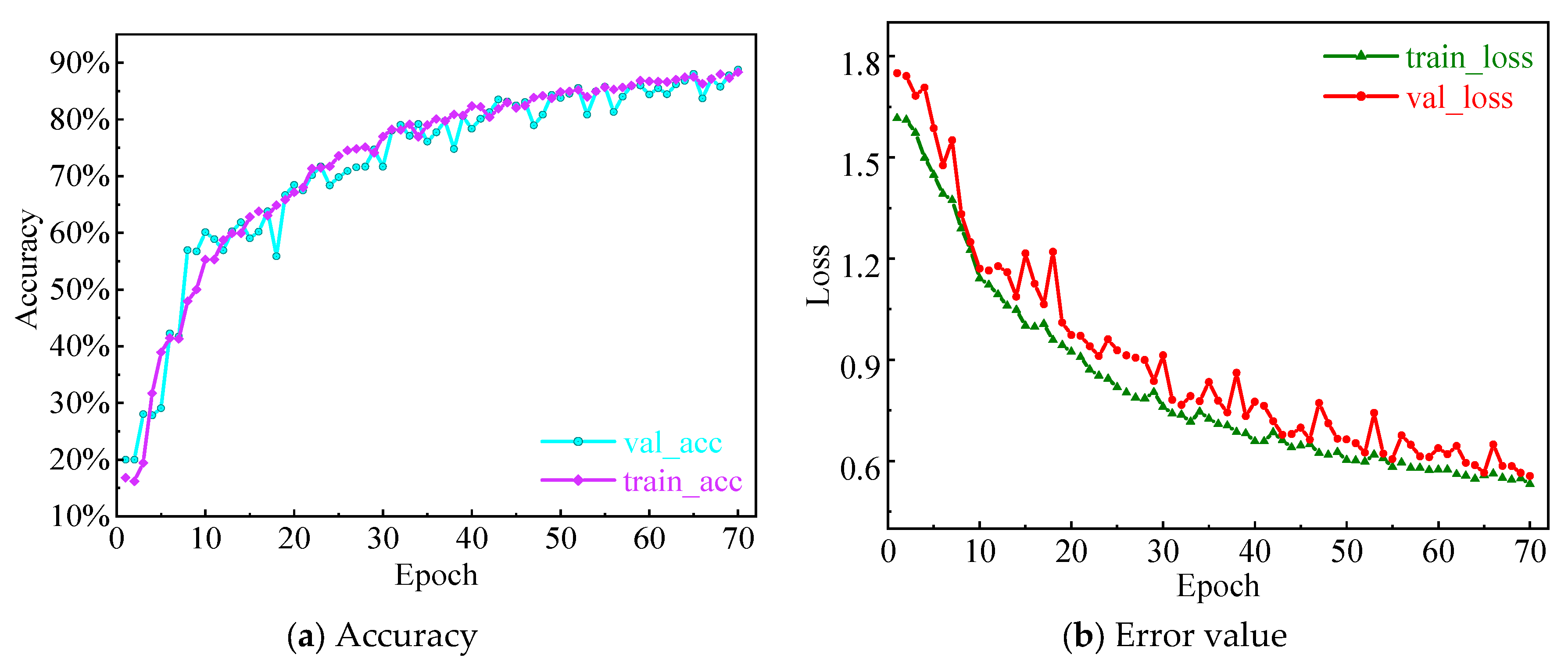
The variation curves of accuracy and error loss corresponding to the training results of the LeNet-5 model are presented in Figure 16. As can be seen from Figure 16a, with the increase in training time, the accuracy rate shows an overall upward trend. The accuracy rate of the training set can reach 90.33%, but the accuracy rate of the verification set is not stable and there are many oscillations. According to Figure 16b, with the increase in training time, the error of the training set keeps decreasing and tends to be level, while the error of the validation set is relatively unstable with visible oscillations.

The variation curves of accuracy and error loss corresponding to the training results of the AlexNet model are displayed in Figure 17. As can be seen from Figure 17a, the accuracy curve increases and converges with the increase in training time. Moreover, the highest accuracy of the training set reaches 88.79%, and the highest accuracy of the validation set reaches 88.59%. Figure 17b shows that the error curve decreases with the increase in training time and finally tends to smooth, with the lowest error of 0.5329 in the validation set and 0.5318 in the training set. The overall performance of the model is relatively stable and the oscillation is not evident.

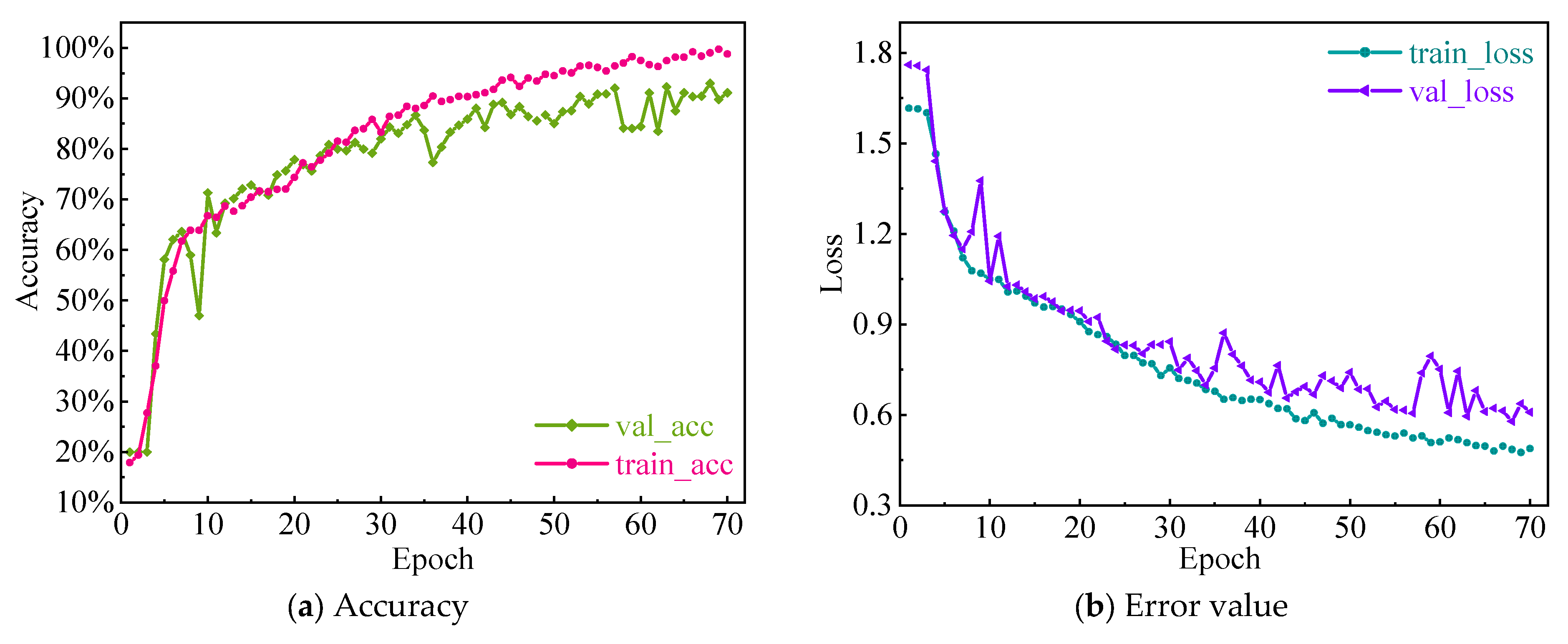
The variation curves of accuracy and error loss corresponding to the training results of the VGG11 model are demonstrated in Figure 18. It can be seen that with the increase in training time, the accuracy of the training set increases gradually, and fluctuates in a small range, up to 92.12%. The accuracy of the validation set gradually increases as a whole, but the performance is not stable in the process of increasing, with an accuracy up to 90.42%. The error loss of the training set gradually decreases and smooths, and the error loss of the validation set gradually decreases but displays several oscillations.

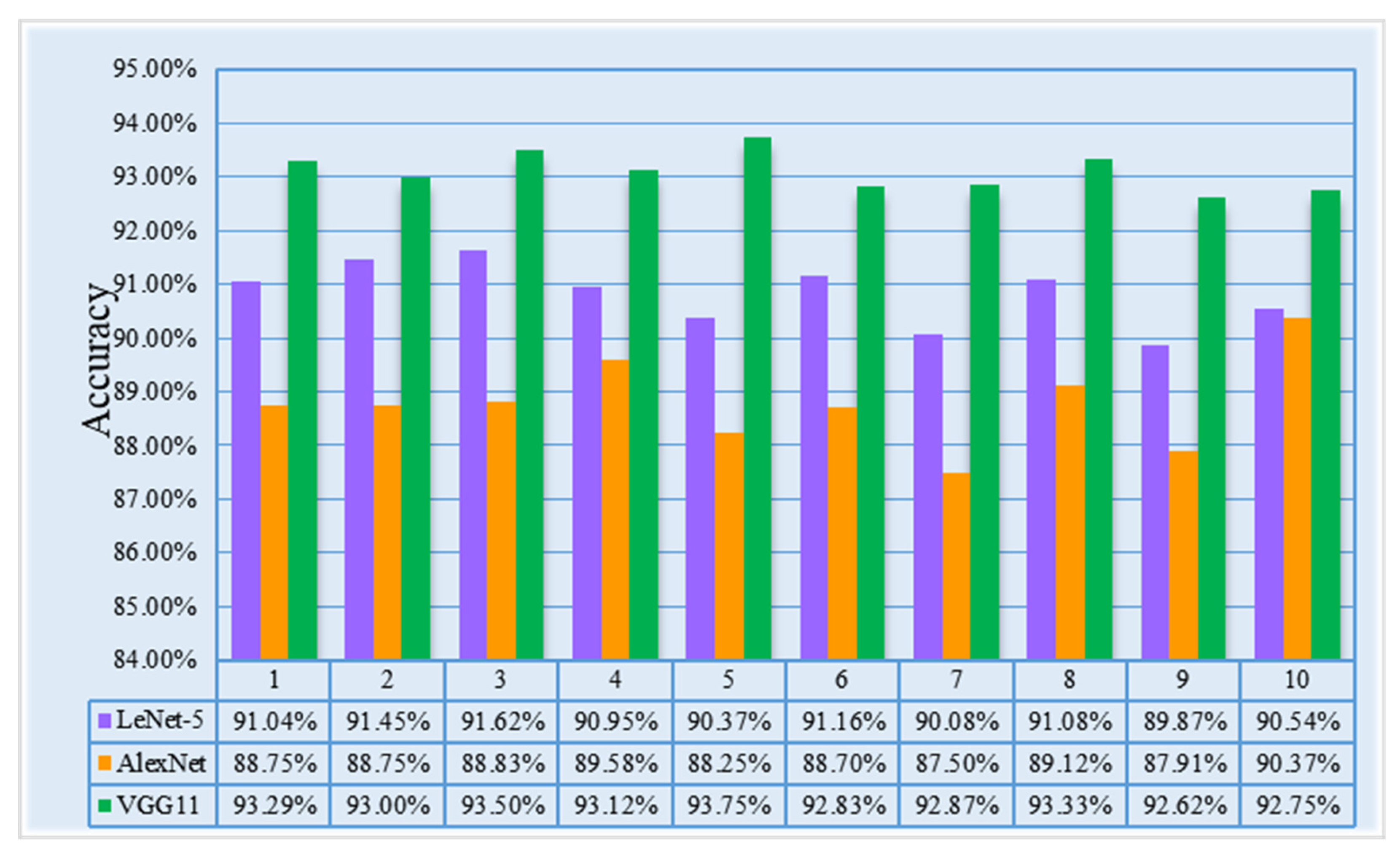
Keeping the hyperparameters of the three classical CNN models unchanged, ten independent repeated trials are performed on the test set. For each calculation, 20% of the samples are randomly selected from the dataset for testing. The test time of the ten repeated experiments of the three classical CNN models is shown in

Table 5. Independent repetition test time of classical CNN models.

Serial Number	1	2	3	4	5	6	7	8	9	10	Average
LeNet-5	0.2279	0.2230	0.2110	0.2200	0.1962	0.1969	0.1901	0.2029	0.2030	0.2030	0.2074
AlexNet	0.4420	0.3539	0.3570	0.3590	0.4339	0.3506	0.3550	0.3539	0.3580	0.3731	0.3736
VGG11	2.9760	3.0180	2.9850	3.2569	3.2395	3.0735	2.7993	2.9649	3.0064	3.0559	3.0375

, and the ten test results are described in Figure 19. From Table 5, the average test time of the LeNet-5 model is 0.2074 s, the average test time of the AlexNet model is 0.3736 s, and the average test time of the VGG11 model is 3.0375 s. It can be seen from Figure 19 that the average value of ten test results of the LeNet-5 model is 90.80%, and the standard deviation is 0.0054. For the AlexNet model, the average value is 88.72% and the standard deviation is 0.0067. For the VGG11 model, the mean value is 93.07% and the standard deviation is 0.0057. Although the test time of the LeNet-5 model and the AlexNet model is shorter than that of the VGG11 model, the accuracy rate is not as high as that of the VGG11 model. By comparing the accuracy, test time, and standard deviation of the three classical CNN models, the overall performance of the VGG11 model is the best.

5.3. Intelligent Fault Diagnosis by Integrating SWT and VGG-LSTM

The training samples and validation samples are input into the established VGG–LSTM fusion model for training, and the model performance is tested by test samples. The optimizer is bound to an exponential decay learning rate controller, and the learning rate is set to 0.001. Each epoch learning rate is multiplied by 0.5 for each 30 steps of training. As the iteration continues, the learning rate is gradually updated, making the model more stable in the later stage of training.

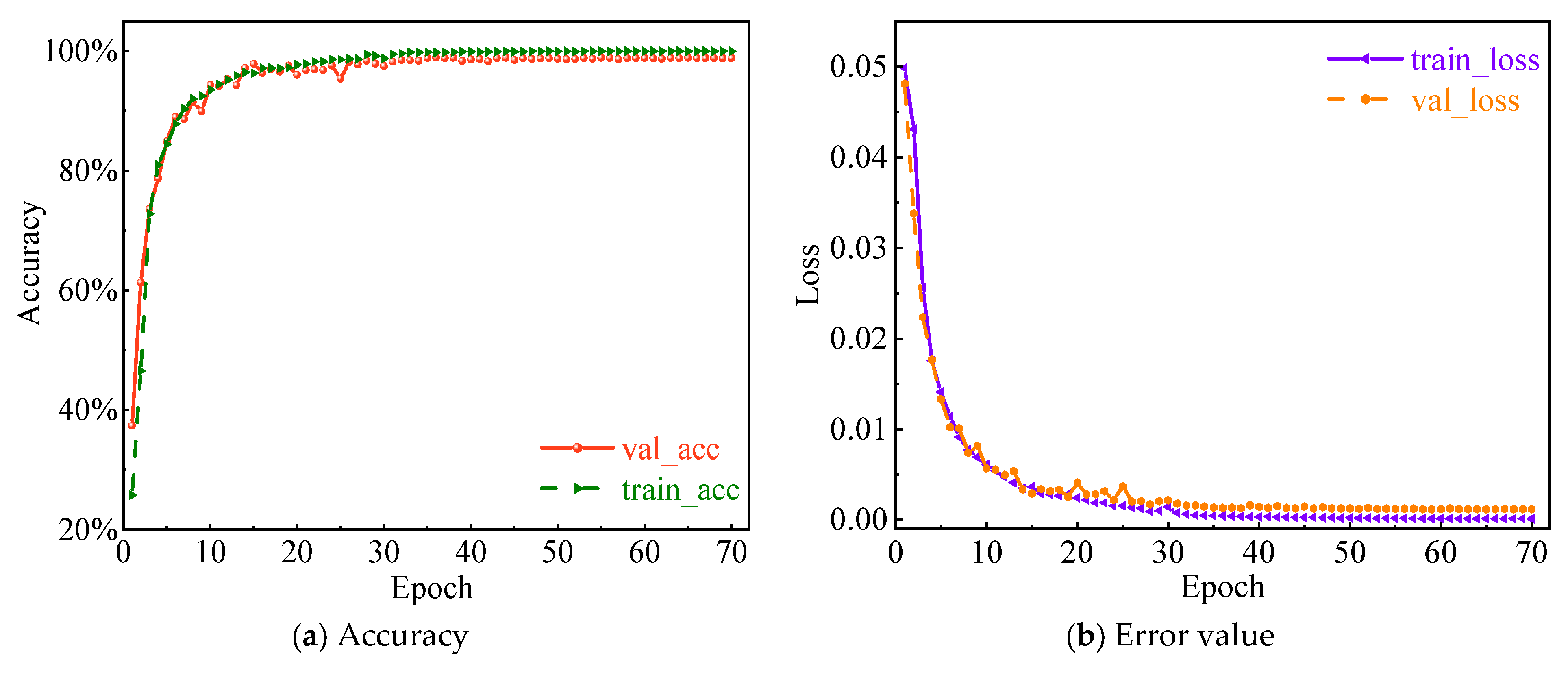
The curves of accuracy and error loss corresponding to the training results of the VGG–LSTM fusion model are presented in Figure 20. In the first 10 trainings, the accuracy rate gradually increased. After 10 trainings, the accuracy curve tended to be stable. The training results of the training set could reach 100%, and the training results of the verification set could reach 99.83%. Similar to the accuracy curve, the error curve rapidly dropped to a stable value in the first 10 trainings. After 10 trainings, the training process is stable, and the error of the training set and the verification set approaches zero. In summary, the VGG–LSTM fusion model has higher identification accuracy and faster convergence speed in the training process.

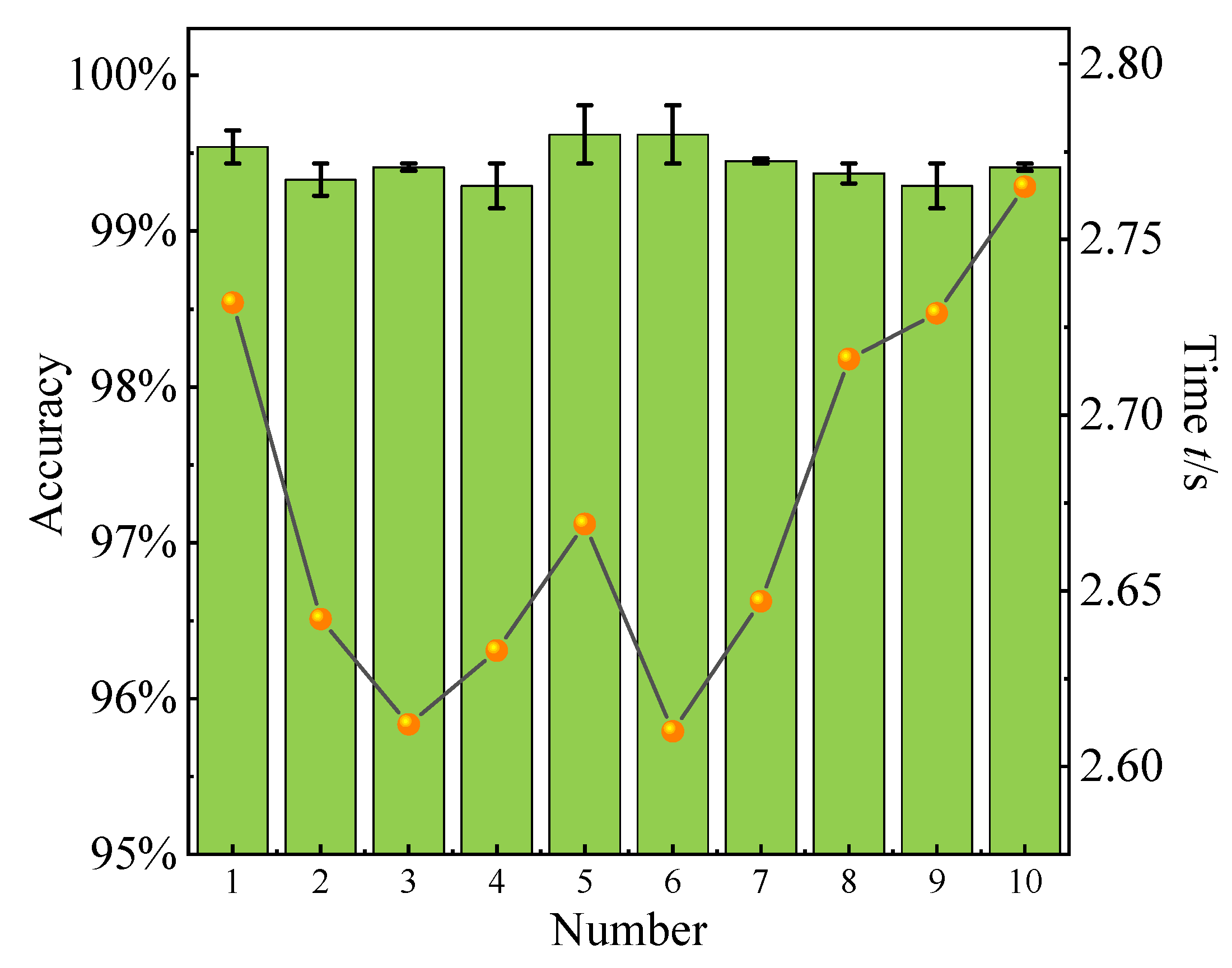
To demonstrate the generalization of the proposed method, 20% of the test set is randomly selected to test the performance of the trained model, and ten independent repeated tests are performed on the test set. The test results are displayed in

Table 6. Repeat test time and accuracy of VGG–LSTM fusion model.

Serial Number	1	2	3	4	5	6	7	8	9	10	Average	Standard Deviation
Test accuracy/%	99.54	99.33	99.41	99.29	99.62	99.62	99.45	99.37	99.29	99.41	99.43	0.0011
Test time/s	2.732	2.642	2.612	2.633	2.669	2.610	2.647	2.716	2.729	2.765	2.675	0.0527

. Combined with Figure 21, the results of ten tests are calculated, the average test accuracy is 99.43%, and the standard deviation of the test accuracy is 0.0011. The average test time is 2.6755 s, and the standard deviation of the test time is 0.0527.

5.4. Comparation Analysis of Different Models

In order to better verify the superiority of the constructed models, a comparison test of the above models is performed. From the perspective of accuracy, error, standard deviation, and time, the above models are comprehensively compared. The details of each model are described in

Table 7. Multi-model comparison.

Model	Single Layer LSTM	Double Layer LSTM	Three-Layer LSTM	LeNet-5	AlexNet	VGG11	VGG-LSTM
Training accuracy/%	85.14	65.32	39.42	90.33	88.79	92.12	100
Training error	0.00645	0.01309	0.02140	0.57240	0.53189	0.48868	0.00011
Average training time/s	14.376	14.221	14.561	40.725	40.265	80.458	41.458
Accuracy of verification/%	78.25	65.29	34.29	89.65	88.76	90.43	99.62
Verification error	0.00788	0.01253	0.02233	0.5649	0.5329	0.60265	0.00013
Average verification time/s	5.373	5.691	5.627	17.899	17.852	23.130	4.771
Average test accuracy/%	70.38	52.06	45.65	90.81	88.77	93.10	99.43
Test standard deviation	0.0056	0.0076	0.0071	0.0054	0.0081	0.0035	0.0011
Average test time/s	1.952	2.091	2.167	0.207	0.373	3.037	2.675
Model parameter	2	3	4	5	8	11	10

.

It can be seen from Table 7, compared with different layers of LSTM models, that the training accuracy, verification accuracy, and average test accuracy of the single-layer LSTM model are the highest. Its training accuracy is 85.14%, the verification accuracy is 78.25%, and the average test accuracy is 70.38%. Compared with the three classical CNN models (LeNet-5, AlexNet, VGG11), the training accuracy, verification accuracy, and average test accuracy of the three models are all above 85%, among which the accuracy of LeNet-5 and VGG11 is higher, and the three accuracy rates are all above 90%, which can better identify the time–frequency diagram of vibration signals of the piston pump. For the VGG–LSTM fusion model, the training accuracy rate is 100%, the verification accuracy rate is 99.62%, and the average test accuracy rate is 99.43%. It has a strong recognition ability and can well identify the five typical states of the axial piston pump.

It can be seen by analyzing the error, the training error, and verification error of the VGG–LSTM fusion model are the lowest, approaching zero, 0.00011, and 0.00013, respectively. Compared with the three classical CNN models, the training error and verification error of the LeNet-5 model are 0.5724 and 0.5649, respectively, the training error and verification error of the AlexNet model are 0.53189 and 0.5329, respectively, and the training error and verification error of the VGG11 model are 0.48868 and 0.60265, respectively. Hence, the training error and verification error of the three classical CNN models are much higher than that of the VGG–LSTM fusion model. Compared with different layers of LSTM models, the training error and verification error of the single-layer LSTM model are 0.00645 and 0.00788, respectively, the training error and verification error of the double-layer LSTM model are 0.01309 and 0.01253, respectively, and the training error and verification error of the three-layer LSTM model are 0.02140 and 0.02233, respectively. Although the error of the LSTM model with different layers is much smaller than that of three classical CNN models, it is still much higher than that of the VGG–LSTM model, and the accuracy of the LSTM model is low.

By analyzing the standard deviation of ten independent repeated tests, the test standard error of the VGG–LSTM fusion model is the lowest, approaching zero, which is 0.0011. Comparing the three classical CNN models, the standard deviations of LeNet-5, AlexNet, and VGG11 are 0.0054, 0.0081, and 0.0035, respectively. The standard deviations of the single-layer LSTM model, two-layer LSTM model, and three-layer LSTM model are 0.0056, 0.0076, and 0.0071, respectively. The results of ten repeated tests show that the VGG–LSTM fusion model has the lowest standard deviation, which indicates that the fusion model is more robust.

From the perspective of time, comparing the average training time, the average training time of LSTM models with different layers is within 20 s, and the average training time of other models is more than 20 s, with the longest training time reaching 80.458 s. The model training process consumes a longer time, among which the training time of the VGG–LSTM fusion model is 41.458 s. Comparing the average validation time, the time of the LSTM models with three different layers are 5.373 s, 5.691 s, and 5.627 s. The average training times of the three classical CNN models are 17.899 s, 17.852 s, and 23.130 s. Additionally, the average validation time of the VGG–LSTM fusion model is 4.771 s. From the average test time of the ten tests, the times of the LSTM models with three different layers are 1.952 s, 2.091 s, and 2.167 s. The average test time of the three classical CNN models are 0.207 s, 0.373 s, and 3.037 s. Additionally, the average test time of the VGG–LSTM fusion model is 2.675 s.

In summary, the VGG–LSTM fusion model has the highest accuracy and the lowest training and verification errors. The average test accuracy of the ten tests is the highest, the standard deviation of the test is the smallest, and the average test time is relatively short. Hence, the comprehensive performance of the VGG–LSTM fusion model is the best, which can effectively achieve the accurate identification of typical faults of an axial piston pump.

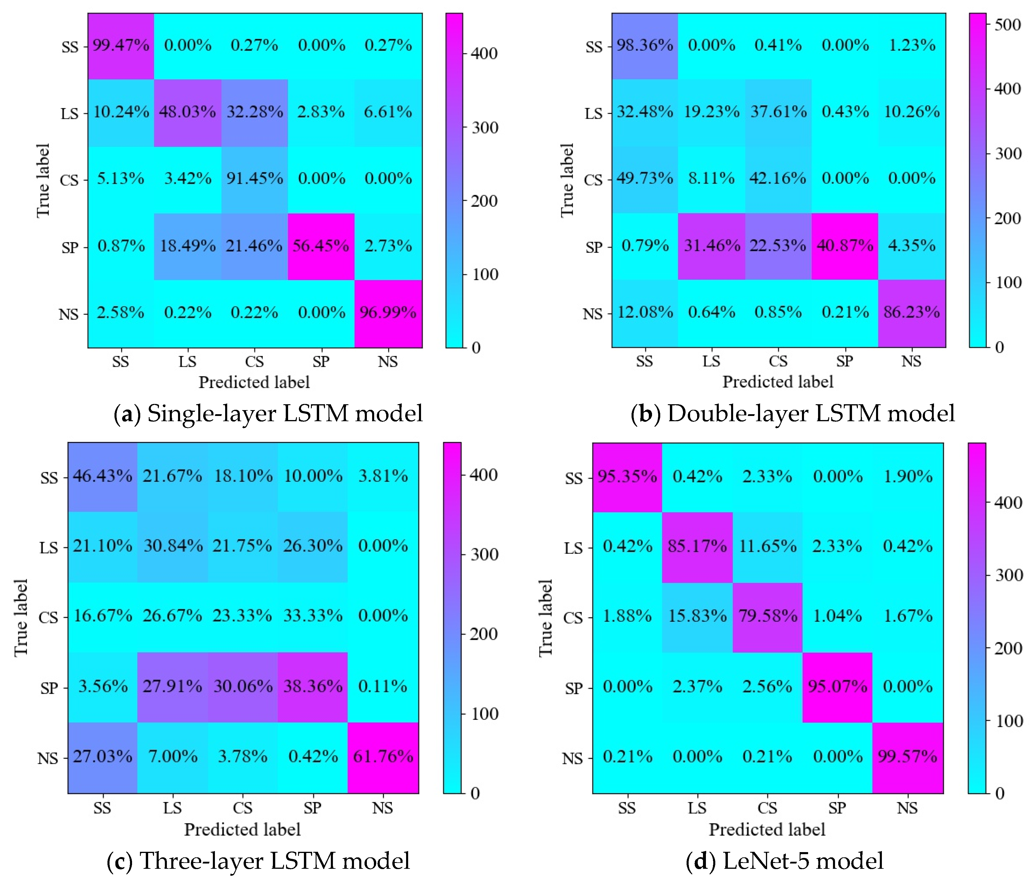
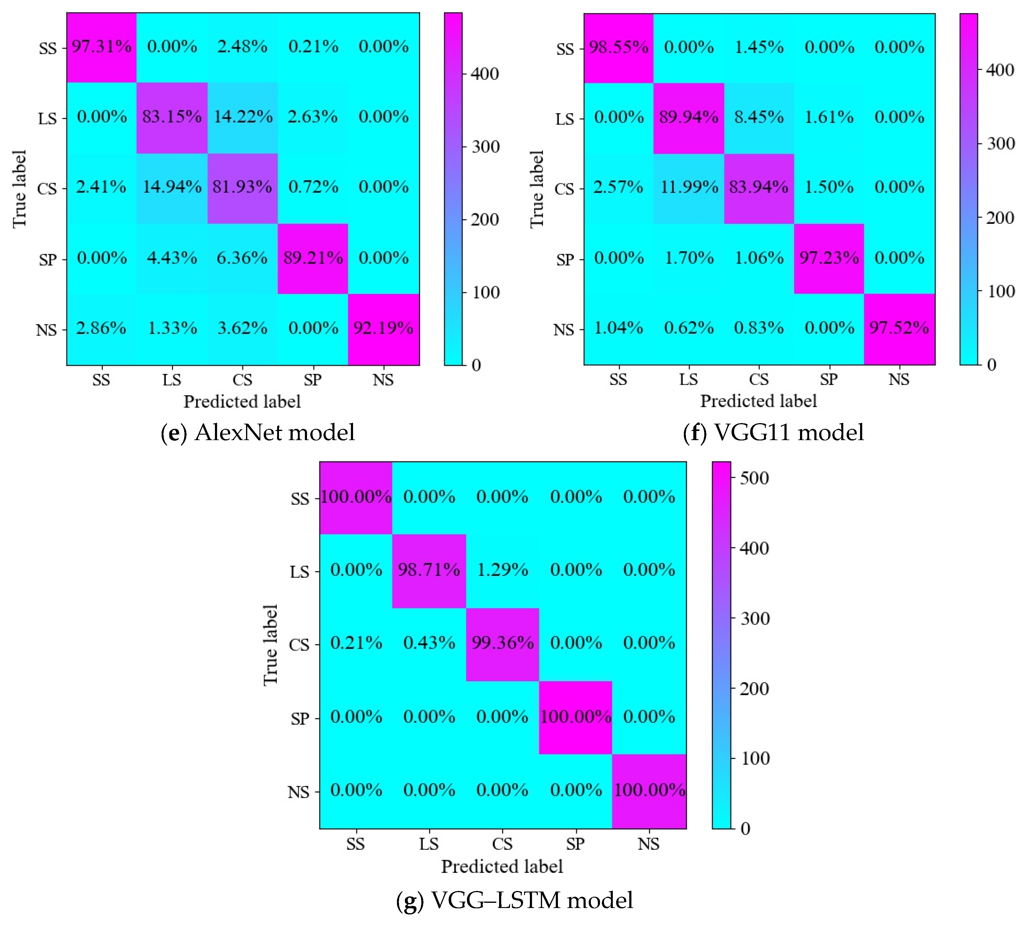
The confusion matrix of each model is generated by reloading the weight file corresponding to the optimal recognition rate, as shown in Figure 22. It can be seen from the confusion matrixes that the LSTM models have low accuracy in identifying the faults of the axial piston pump. The four models of LeNet-5, AlexNet, VGG11, and VGG–LSTM can accurately identify the three states such as slipper wear, swash plate wear, and normal state. The VGG–LSTM model has the highest accuracy, and the recognition accuracy for the above three typical states is 100%. For another two fault states such as loose slipper and center spring failure, several models have some misclassification phenomenon. Commendably, the VGG–LSTM model has the lowest misclassification rate, only 1.29% of loose slipper failures are misidentified as center spring failures, and 0.43% of center spring failures are misidentified as loose slipper failures.

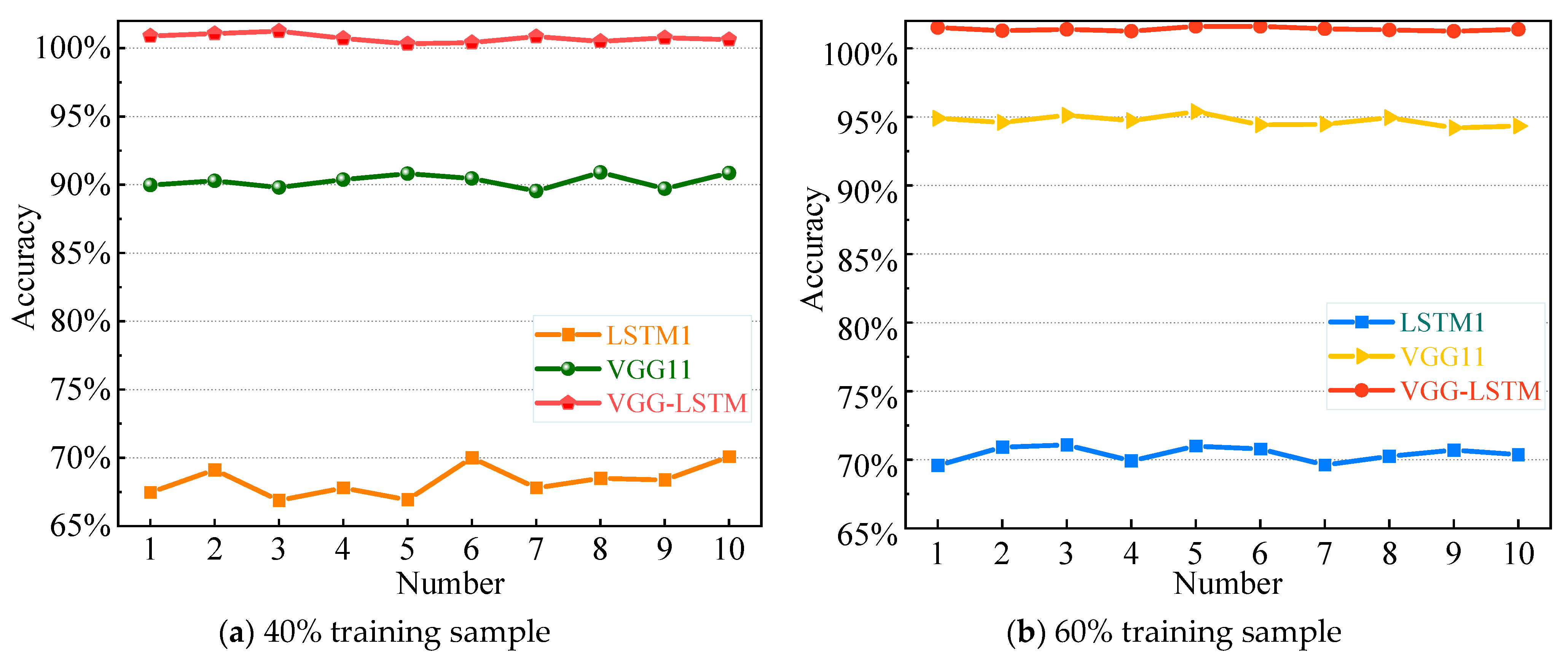
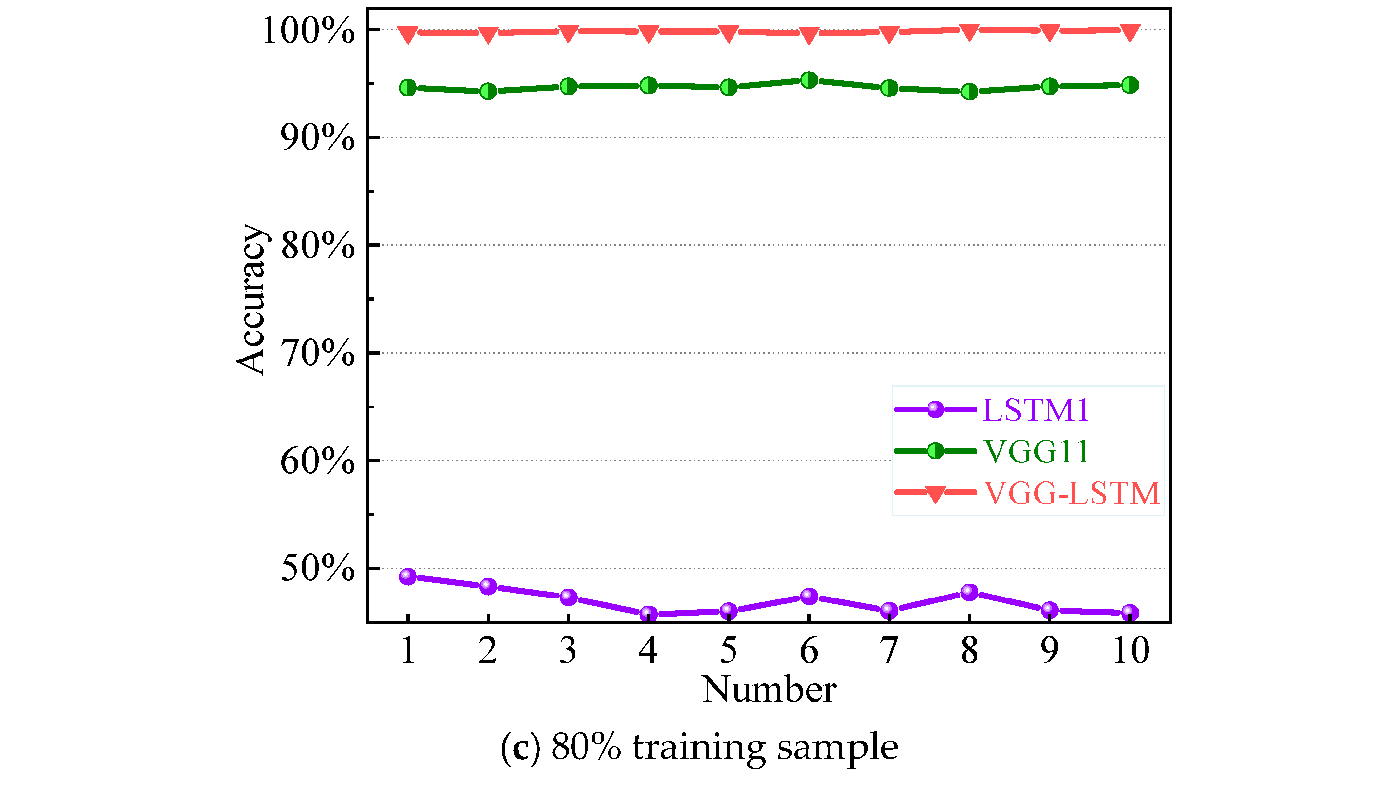
Then, the VGG–LSTM fusion model is further cross-validated with the two better-performing models, including LSTM and VGG11, by setting different training ratios of 40% (4:3:3), 60% (6:2:2), and 80% (8:1:1). The average diagnosis results of the three models under different training ratios are displayed in

Table 8. Multi-model results under different training ratios.

	Model	Index	Single Layer LSTM	VGG11	VGG–LSTM
Proportion
40% training		Training accuracy/%	85.56	86.66	99.95
		Accuracy of verification/%	82.80	76.79	98.05
		Training time/s	9.5185	45.117	34.132
		Authentication time/s	8.112	26.48	7.666
60% training		Training accuracy/%	86.41	92.12	100
		Accuracy of verification/%	80.25	81.14	98.79
		Training time/s	14.376	57.328	41.458
		Authentication time/s	5.373	23.131	4.772
80% training		Training accuracy/%	87.91	94.83	100
		Accuracy of verification/%	83.33	83.17	99.08
		Training time/s	18.859	72.487	55.250
		Authentication time/s	2.476	21.942	2.624

, and the comparison results of ten independent repeated tests are shown in Figure 23.

As can be seen from Table 8, compared with single-layer LSTM and VGG11, the VGG–LSTM fusion model has the highest accuracy rate of fault diagnosis at different training ratios. In terms of program running time, the verification time of the VGG–LSTM fusion model is much faster than that of VGG11. Through Figure 23, it is evident that the accuracy of the proposed VGG–LSTM fusion model is higher than that of the VGG11 model and the single-layer LSTM model, and the results of ten independent tests are also more stable compared to the above two models.

6. Conclusions

To achieve an intelligent fault diagnosis of a hydraulic piston pump, a combined model based on SWT and VGG–LSTM is proposed. The correlation in the original vibration signal is carefully explored, and the diagnosis accuracy of the common faults of a hydraulic axial piston pump is enhanced by integrating the translation invariance of a CNN in time–space and the memory capacity of an RNN. The following findings are obtained:

(1) The SWT method is used for the establishment of a data sample library and transforms 1D vibration signals into 2D time–frequency maps, giving a good input of a diagnostic model. The proposed VGG–LSTM diagnosis model combines the advantages of the single-layer LSTM network model and the VGG11 network model, and has great stability. Meanwhile, it can resolve the long training time of the VGG11 model and the low diagnostic accuracy of the LSTM model. It provides a novel approach for the intelligent fault diagnosis of a hydraulic axial piston pump.

(2) Some classic methods are employed to identify the five typical states by using the measured vibration signals of a hydraulic axial piston pump. The recognition accuracy of the single-layer LSTM model is 85.14%, and the recognition accuracy of the standard VGG11 model is 92.12%. The proposed VGG–LSTM fusion model is rebuilt by integrating the advantages of the VGG11 model and the single-layer LSTM model. The layered learning rate is configured to increase the recognition accuracy of the fusion model up to 100%. The VGG–LSTM fusion model has higher fault recognition accuracy when compared to some classic models such as single-layer LSTM, two-layer LSTM, three-layer LSTM, LeNet-5, AlexNet, and VGG11. It has lower training and validation errors, faster learning and training speeds, and a shorter testing time.

(3) The failure data of a hydraulic axial piston pump are time series data with temporality. The VGG–LSTM fusion model reduces the diagnosis time by utilizing the potent timing processing capabilities of LSTM. The training time of the fusion model is 15.87 s faster than that of the VGG11 model under identical operating conditions. However, when the single-layer LSTM and VGG11 models are combined, the ability of the LSTM model to mine features is improved, while the VGG11 model’s reliance on the number of data samples is lessened. The effective information buried in the temporal data is mined in conjunction with the prospective feature extraction capability of the VGG11 model, the diagnostic accuracy and effectiveness of the common faults of the hydraulic axial piston pump are improved.

The approach can further be explored as a method for the intelligent fault diagnosis of other rotating machinery such as motors, gears, bearings, and so on. The following work can be explored in the future:

(1) The effect of the VGG–LSTM model on fault identification of hydraulic axial piston pumps under variable speed.

(2) The number of layers of the VGG–LSTM fusion model can be reduced so as to further optimize the model.

(3) The influence of different sampling frequencies on the results of the fusion diagnosis method.

References

1. Ai, C.; Zhang, L.; Gao, W.; Yang, G.; Wu, D.; Chen, L.; Chen, W.; Plummer, A. A review of energy storage technologies in hydraulic wind turbines. Energ. Convers. Manag. 2022, 264, 115584. [Google Scholar] [CrossRef]
2. Cheng, N.; Gao, X.; Wang, L.; Liu, Y. Design, analysis and testing of a hydraulic catapult system. IEEE Access 2022, 10, 67482–67492. [Google Scholar] [CrossRef]
3. Wang, F.; Chen, J.; Cheng, M.; Xu, B. A novel hydraulic transmission solution to large offshore wind turbine: Design and control strategy. Ocean Eng. 2022, 255, 111285. [Google Scholar] [CrossRef]
4. Gao, Q.; Zhu, Y.; Liu, J. Dynamics modelling and control of a novel fuel metering valve actuated by two binary-coded digital valve arrays. Machines 2022, 10, 55. [Google Scholar] [CrossRef]
5. Banaszek, A.; Petrovic, R.; Andjelkovic, M.; Radosavljevic, M. The concept of efficiency of a twin-two-pump hydraulic power pack with pumps equipped in constant pressure regulators with different linear I performance characteristics. Energies 2022, 15, 8100. [Google Scholar] [CrossRef]
6. Tang, S.; Zhu, Y.; Yuan, S. Intelligent fault identification of hydraulic pump using deep adaptive normalized CNN and synchrosqueezed wavelet transform. Relia. Eng. Syst. Saf. 2022, 224, 108560. [Google Scholar] [CrossRef]
7. Banaszek, A.; Petrovic, R. Problem of non proportional flow of hydraulic pumps working with constant pressure regulators in big power multipump power pack unit in open system. Teh. Vjesn. 2019, 26, 294–301. [Google Scholar]
8. Ye, S.; Zhang, J.; Xu, B.; Hou, L.; Xiang, J.; Tang, H. A theoretical dynamic model to study the vibration response characteristics of an axial piston pump. Mech. Syst. Signal Pract. 2020, 150, 107237. [Google Scholar] [CrossRef]
9. Tang, S.; Zhu, Y.; Yuan, S. A novel adaptive convolutional neural network for fault diagnosis of hydraulic piston pump with acoustic images. Adv. Eng. Inform. 2022, 52, 101554. [Google Scholar] [CrossRef]
10. Chao, Q.; Xu, Z.; Tao, J.; Liu, C. Capped piston: A promising design to reduce compressibility effects, pressure ripple and cavitation for high-speed and high-pressure axial piston pumps. Alex. Eng. J. 2023, 62, 509–521. [Google Scholar] [CrossRef]
11. Qian, P.; Pu, C.; Liu, L.; Lv, P.; Páez, L.M.R. A novel pneumatic actuator based on high-frequency longitudinal vibration friction reduction. Sens. Actuat. A-Phys. 2022, 344, 113731. [Google Scholar] [CrossRef]
12. Zuo, C.; Qian, J.; Feng, S.; Yin, W.; Li, Y.; Fan, P.; Han, J.; Qian, K.; Chen, Q. Deep learning in optical metrology: A review. Light Sci. Appl. 2022, 11, 1–54. [Google Scholar] [CrossRef]
13. Pang, Y.; Bai, X.; Zhang, G. Special focus on deep learning for computer vision. Sci. China Inform. Sci. 2020, 63, 120100. [Google Scholar] [CrossRef] [Green Version]
14. Huang, S.; Luo, S.; Yang, Y.; Li, T.; Wu, Y.; Zeng, Q.; Huang, H. Determination of optical rotation based on liquid crystal polymer vortex retarder and digital image processing. IEEE Access 2022, 10, 8219–8226. [Google Scholar] [CrossRef]
15. Zhao, M.; Fu, X.; Zhang, Y.; Meng, L.; Zhong, S. Data augmentation via randomized wavelet expansion and its application in few-shot fault diagnosis of aviation hydraulic pumps. IEEE Trans. Instrum. Meas. 2021, 71, 1–13. [Google Scholar] [CrossRef]
16. Wang, S.; Jia, W. A minimum entropy deconvolution-enhanced convolutional neural networks for fault diagnosis of axial piston pumps. Soft Comput. 2020, 24, 2983–2997. [Google Scholar] [CrossRef]
17. He, Y.; Tang, H.; Ren, Y.; Kumar, A. A deep multi-signal fusion adversarial model based transfer learning and residual network for axial piston pump fault diagnosis. Measurement 2022, 192, 110889. [Google Scholar] [CrossRef]
18. Chao, Q.; Wei, X.; Lei, J.; Tao, J.; Liu, C. Improving accuracy of cavitation severity recognition in axial piston pumps by denoising time-frequency images. Meas. Sci. Technol. 2022, 33, 055116. [Google Scholar] [CrossRef]
19. Chao, Q.; Gao, H.; Tao, J.; Wang, Y.; Zhou, J.; Liu, C. Adaptive decision-level fusion strategy for the fault diagnosis of axial piston pumps using multiple channels of vibration signals. Sci. China: Technol. Sci. 2022, 65, 470–480. [Google Scholar] [CrossRef]
20. Tang, S.; Zhu, Y.; Yuan, S. Intelligent fault diagnosis of hydraulic piston pump based on deep learning and bayesian optimization. ISA Trans. 2022, 129, 555–563. [Google Scholar] [CrossRef]
21. Tang, S.; Zhu, Y.; Yuan, S. An adaptive deep learning model towards fault diagnosis of hydraulic piston pump using pressure signal. Eng. Failure Anal. 2022, 138, 106300. [Google Scholar] [CrossRef]
22. Zhu, Y.; Li, G.; Wang, R.; Tang, S.; Su, H.; Cao, K. Intelligent fault diagnosis of hydraulic piston pump combining improved LeNet-5 and PSO hyperparameter optimization. Appl. Acoust. 2021, 183, 108336. [Google Scholar] [CrossRef]
23. Zhu, Y.; Li, G.; Tang, S.; Wang, R.; Su, H.; Wang, C. Acoustic signal-based fault detection of hydraulic piston pump using a particle swarm optimization enhancement CNN. Appl. Acoust. 2022, 192, 108718. [Google Scholar] [CrossRef]
24. Sinitsin, V.; Ibryaeva, O.; Sakovskaya, V.; Eremeeva, V. Intelligent bearing fault diagnosis method combining mixed input and hybrid CNN-MLP model. Mech. Syst. Signal. Process. 2022, 180, 109454. [Google Scholar] [CrossRef]
25. Choudhary, A.; Mishra, R.; Fatima, S.; Panigrahi, B.K. Multi-input CNN based vibro-acoustic fusion for accurate fault diagnosis of induction motor. Eng. Appl. Artif. Intell. 2023, 120, 105872. [Google Scholar] [CrossRef]
26. Glowacz, A. Thermographic fault diagnosis of shaft of BLDC motor. Sensors 2022, 22, 8537. [Google Scholar] [CrossRef]
27. Dibaj, A.; Ettefagh, M.; Hassannejad, R.; Ehghaghi, M. A hybrid fine-tuned VMD and CNN scheme for untrained compound fault diagnosis of rotating machinery with unequal-severity faults. Expert Syst. Appl. 2021, 167, 114094. [Google Scholar] [CrossRef]
28. Andayani, F.; Theng, L.B.; Tsun, M.T.; Chua, C. Hybrid LSTM-transformer model for emotion recognition from speech audio files. IEEE Access 2022, 10, 36018–36027. [Google Scholar] [CrossRef]
29. Xu, H.; Hu, B. Legal text recognition using LSTM-CRF deep learning model. Comput. Intel. Neurosc. 2022, 2022, 1–10. [Google Scholar] [CrossRef]
30. Zhu, Y.; Zhu, C.; Tan, J.; Wang, Y.; Tao, J. Operational state assessment of wind turbine gearbox based on long short-term memory networks and fuzzy synthesis. Renew. Energ. 2022, 181, 1167–1176. [Google Scholar] [CrossRef]
31. Zhu, Y.; Zhu, C.; Tan, J.; Tan, Y.; Rao, L. Anomaly detection and condition monitoring of wind turbine gearbox based on LSTM-FS and transfer learning. Renew. Energ. 2022, 189, 90–103. [Google Scholar] [CrossRef]
32. Sun, H.; Zhao, S. Fault diagnosis for bearing based on 1DCNN and LSTM. Shock Vib. 2021, 2021, 1–17. [Google Scholar] [CrossRef]
33. Bie, F.; Du, T.; Lyu, F.; Pang, M.; Guo, Y. An integrated approach based on improved CEEMDAN and LSTM deep learning neural network for fault diagnosis of reciprocating pump. IEEE Access 2021, 9, 23301–23310. [Google Scholar] [CrossRef]
34. Zhao, Q.; Cheng, G.; Han, X.; Liang, D.; Wang, X. Fault diagnosis of main pump in converter station based on deep neural network. Symmetry 2021, 13, 1284. [Google Scholar] [CrossRef]
35. Khan, M.M.; Tse, P.W.; Trappey, A.J. Development of a novel methodology for remaining useful life prediction of industrial slurry pumps in the absence of run to failure data. Sensors 2021, 21, 8420. [Google Scholar] [CrossRef]
36. Du, J.; Li, X.; Gao, Y.; Gao, L. Integrated gradient-based continuous wavelet transform for bearing fault diagnosis. Sensors 2022, 22, 8760. [Google Scholar] [CrossRef]
37. Daubechies, I.; Lu, J.; Wu, H.T. Synchrosqueezed wavelet transforms: An empirical mode decomposition-like tool. Appl. Comput. Harmon. A 2011, 30, 243–261. [Google Scholar] [CrossRef] [Green Version]
38. Lee, S.; Kim, H.; Lieu, Q.X.; Lee, J. CNN-based image recognition for topology optimization. Knowl. Based Syst. 2020, 198, 105887. [Google Scholar] [CrossRef]
39. Cooney, C.; Korik, A.; Folli, R.; Coyle, D. Evaluation of hyperparameter optimization in machine and deep learning methods for decoding imagined speech EEG. Sensors 2020, 20, 4629. [Google Scholar] [CrossRef]
40. Wang, T.; Lu, C.; Shen, G.; Hong, F. Sleep apnea detection from a single-lead ECG signal with automatic feature-extraction through a modified LeNet-5 convolutional neural network. PeerJ 2019, 7, 1–17. [Google Scholar] [CrossRef] [Green Version]
41. Lu, T.; Han, B.; Yu, F. Detection and classification of marine mammal sounds using AlexNet with transfer learning. Ecol. Inform. 2021, 62, 101277. [Google Scholar] [CrossRef]
42. Zhang, D.; Lv, J.; Cheng, Z. An approach focusing on the convolutional layer characteristics of the VGG network for vehicle tracking. IEEE Access 2020, 8, 112827–112839. [Google Scholar] [CrossRef]
43. Shao, S.; McAleer, S.; Yan, R.; Baldi, P. Highly accurate machine fault diagnosis using deep transfer learning. IEEE T. Ind. Inform. 2018, 15, 2446–2455. [Google Scholar] [CrossRef]
44. Jiao, J.; Zhao, M.; Lin, J.; Liang, K. A comprehensive review on convolutional neural network in machine fault diagnosis. Neurocomputing 2020, 417, 36–63. [Google Scholar] [CrossRef]
45. Majumdar, A.; Gupta, M. Recurrent transform learning. Neural Netw. 2019, 118, 271–279. [Google Scholar] [CrossRef] [Green Version]
46. Zhu, F.; Liang, Q. Rethink of orthographic constraints on RNN and its application in acoustic sensor data modeling. IEEE Internet Things J. 2021, 9, 1962–1975. [Google Scholar] [CrossRef]
47. Carrasco, M.; Barbot, A. Spatial attention alters visual appearance. Curr. Opin. Psychol. 2019, 29, 56–64. [Google Scholar] [CrossRef] [Green Version]
48. Kasera, R.K.; Acharjee, T. Parking slot occupancy prediction using LSTM. Innov. Syst. Softw. Eng. 2022, 1–13. [Google Scholar] [CrossRef]
49. Zhao, X.; Jin, X. A comparative study of text genres in english-chinese translation effects based on deep learning LSTM. Comput. Math. Method. Med. 2022, 2022, 1–9. [Google Scholar] [CrossRef]
50. Tang, Z. Music sense analysis of bel canto audio and bel canto teaching based on LSTM mixed model. Mob. Inf. Syst. 2022, 2022, 1–8. [Google Scholar] [CrossRef]
51. Yang, J.; Peng, Y.; Xie, J.; Wang, P. Remaining useful life prediction method for bearings based on LSTM with uncertainty quantification. Sensors 2022, 22, 4549. [Google Scholar] [CrossRef]
52. Shi, J.; Peng, D.; Peng, Z.; Zhang, Z.; Goebel, K.; Wu, D. Planetary gearbox fault diagnosis using bidirectional-convolutional LSTM networks. Mech. Syst. Signal Pract. 2022, 162, 107996. [Google Scholar] [CrossRef]
Figure 1. Application of hydraulic system.
Jmse 11 00594 g001
Figure 2. Schematic diagram of the structure of network model.
Jmse 11 00594 g002
Figure 3. Schematic diagram of convolution calculation.
Jmse 11 00594 g003
Figure 4. Schematic diagram of maximum pooling.
Jmse 11 00594 g004
Figure 5. Structure sketch of LSTM network model.
Jmse 11 00594 g005
Figure 6. Sketch of model structure of VGG–LSTM network.
Jmse 11 00594 g006
Figure 7. Diagnosis flow chart of VGG–LSTM network.
Jmse 11 00594 g007
Figure 8. Test system of hydraulic axial piston pump.
Jmse 11 00594 g008
Figure 9. Photos of typical faulty components.
Jmse 11 00594 g009aJmse 11 00594 g009b
Figure 10. Basic structure diagram of a hydraulic axial piston pump.
Jmse 11 00594 g010
Figure 11. Time domain diagrams of vibration signals of five typical states.
Jmse 11 00594 g011aJmse 11 00594 g011b
Figure 12. Time–frequency diagrams of vibration signals of five typical states.
Jmse 11 00594 g012
Figure 13. Sample library composition at 5 MPa working pressure.
Jmse 11 00594 g013
Figure 14. Comparison results of different LSTM models.
Jmse 11 00594 g014
Figure 15. Repeat test results of the single-layer LSTM model.
Jmse 11 00594 g015
Figure 16. Training results of LeNet-5 model.
Jmse 11 00594 g016
Figure 17. Training results of AlexNet model.
Jmse 11 00594 g017
Figure 18. Training results of VGG11 model.
Jmse 11 00594 g018
Figure 19. Repeat test results of classical CNN models.
Jmse 11 00594 g019
Figure 20. Training results of VGG–LSTM fusion model.
Jmse 11 00594 g020
Figure 21. Repeat test results of VGG–LSTM fusion model.
Jmse 11 00594 g021
Figure 22. Confusion matrix of optimal test of each model.
Jmse 11 00594 g022aJmse 11 00594 g022b
Figure 23. Repeated test results of multiple models with different training ratios.
Jmse 11 00594 g023aJmse 11 00594 g023b