1. Introduction
Although large seagoing ships usually sail in deep waters, with the increase in ship dimensions and waterway traffic in restricted water, not so rare are situations with two ships moving in close proximity in rivers and channels, in which case the boundary conditions cause a significant change in the flow about the ships and produce additional forces on the hull. A typical case of two ships moving in close proximity in shallow water is two ships moving on parallel courses, either overtaking or head-on encountering. Such cases have been studied experimentally and numerically by researchers in the past decades.
The research methods of ship hydrodynamic interaction can be categorized into model experimentation and numerical simulation. In recent years, researchers have carried out a series of ship model experiments and provided a wealth of experimental data. Relatively comprehensive constrained model tests were carried out by Vantorre et al. [
1], who obtained the hydrodynamic interaction forces from the cross tests of four ship models and analyzed the influence of ship speed, water depth, lateral distance and other configurations. Based on this, an empirical formula for hydrodynamic calculation was derived.
Through model tests, Sano et al. [
2] studied the hydrodynamic forces of ships in restricted waters for various ship–shore distances and drift angles, and, based on regression, an empirical formula for hydrodynamic interaction was obtained and a model for calculating ship motion accounting for the ship–shore interaction was proposed.
Experimental methods are, in general, reliable and accurate, and they are widely used for the investigation of ship hydrodynamic interaction effects and for the validation of numerical methods. However, experimental methods usually require much higher cost and more time, and only a very limited number of motions can be simulated in the towing tank. In contrast, numerical methods do not have these restrictions and sometimes are less costly and time-consuming.
Based on the classic Hess Smith method, Sutulo and Guedes Soares [
3] developed an algorithm for fast calculation of ship hydrodynamic interaction forces and carried out a series of studies on the problem of ship–ship hydrodynamic interaction including extensive validation [
4]. The algorithm was then integrated with the ship maneuvering equation for the simulation of the motion response and trajectory of the two ships accounting for the hydrodynamic interaction forces [
5]. By applying the mirror image technique and a paneled moving patch technique, the algorithm was also extended to deal with the hydrodynamic interaction problem of ships moving in shallow water over a horizontal flat bottom [
6] and in restricted waters with complex boundaries [
7].
To investigate the influence of propulsors on the changes in the flow about the ship as well as the resulting hydrodynamic interacting forces acting on the hulls of two ships moving in close proximity, Sutulo and Guedes Soares [
8] adopted the activation disk model to simulate the propeller at the rear of the hull. The rotation of the propeller generated an axial induced velocity of flow, while the influence of tangential induced velocity and slipstream were neglected. Based on the analysis of the numerical results for the case of overtaking conditions, it was concluded that the influence of propellers is negligible compared with the interaction force produced by the moving body of the hull in proximity. Degrieck et al. [
9] compared two potential-flow-based methods (including the calculation program developed by Sutulo et al. [
6]), CFD methods, and test results for ship–ship and ship–bank hydrodynamic interaction. The comparison showed that the influence of a propeller revealed by both potential flow algorithms is negligible; significant discrepancies between the potential flow results and the CFD simulations\experimental results were observed and they were attributed to the influence of propellers. The study showed that the propeller effect may not be neglected in the ship–ship hydrodynamic interaction, but in-depth study of the propeller’s effect on the pressure distribution on the hull and on the hydrodynamic interaction forces was not presented.
Viscous flow numerical methods, especially RANSE-based ones, have also been adopted by many researchers to study the ship hydrodynamic interaction problem. Yang et al. [
10] applied a RANSE-based method to study ship hydrodynamic interaction with the Wigley and KVLCC2 models, and comparison with the numerical results obtained with potential flow methods showed a good agreement for low-Froude-number cases. Zou and Larsson [
11] carried out numerical simulations of ship hydrodynamic interaction during lightering operation. The influence of water depth, speed, and relative position between ships were analyzed, and the wave pattern, pressure distribution, and hydrodynamic force were obtained. Wnęk et al. [
12] performed a numerical study on the hydrodynamic interaction between tug and tanker, and it was found that the wavemaking effect may play an important role when the clearance between the two vessels is small. There exist more RANSE-based studies of ship–ship hydrodynamic interaction, but none of them have analyzed the propeller effect.
The hydrodynamic interaction effect has also been studied for the case of a moored ship and a passing ship, for instance, in the studies of Pawar et al. [
13] and Zhou et al. [
14]; however, the propeller effect was neglected in these works. To model the propeller in RANSE-based simulations, the volumetric force propeller model has been widely used. Feng et al. [
15] based on the volumetric force propeller model, a method coupled the blade element momentum theory (BEMT) considering the three-dimensional viscous effects with the RANS solvers was adopted to simulate the stern propeller, and the numerical results were in good agreement with the experiment. Dhinesh et al. [
16] and Queutey et al. [
17] adopted the slip grid technique to simulate the rotation of the propeller through the rotation of the grid and obtained the wake field of propeller. There also exists a numerical study of ship–bank hydrodynamic interaction where the propeller is modeled in a RANSE-based simulation. Van Hoydonck et al. [
18] conducted a study on the ship–shore effect, and the propeller and rudder were modeled in RANSE-based numerical simulations; the hydrodynamic forces were obtained. The wave elevation between the ship and the shore wall was analyzed, and it was concluded that the effect of the propeller amplifies the bank effects.
It can be seen from the review of existing studies that, although the propeller effect may be significant in the problem of ship–ship hydrodynamic interaction, the understanding of its contribution and behavioral pattern is very limited. The present study aims at the analysis of the characteristics of the propeller’s effect in ship–ship hydrodynamic interaction. A series of numerical simulations of near-field hydrodynamic interaction of ships moving at zero speed is carried out, and the interaction force, hull surface pressure, and wave elevation are obtained. In most of the realistic scenarios of ship–ship hydrodynamic interaction, at least one of the interacting ships is moving at non-zero speeds, but it is more reasonable to start the study with the case of both ships moving at zero speeds for two reasons: (1) the zero speed case, which excludes the speed factor, is an approach to isolate the propeller effect from a complex hydrodynamic interaction problem; and (2) the understanding of the propeller effect in hydrodynamic interaction between two ships at zero speed will greatly help to reveal the propeller effect in non-zero-speed cases.
2. Problem Formulation
Based on the RANSE viscous flow numerical simulation method, the effect of the propeller on ship–ship hydrodynamic interaction in shallow water is studied. The fluid flow around the hull caused by propeller rotation is considered as an unsteady flow of incompressible viscous fluid, and there are no other external disturbances. The code Star CCM+ 14.02.012 is used to simulate the turbulent viscous flow around the interacting ships and solve the RANS equations. In order to reveal the propeller effect, excluding the contribution of the ship wake, the case of both interacting ships moving at zero speed is investigated in this study. A hull equipped with a propeller and a bare hull are used for the numerical simulation and analysis. The hull with a propeller is a source of hydrodynamic interaction and is named as SOD. The bare hull is the interfered ship, which is referred to as DS. The flow field around the hulls is disturbed by rotation of the propeller, generating hydrodynamic interaction forces and moments. The influences of the speed of the propeller, water depth, lateral distance, and the longitudinal position of the ships are investigated.
2.1. Definitions of Coordinate Systems
The body-fixed coordinate systems
and
are attached to SOD and DS, respectively, where the
axis is pointing forward, the
axis is directed to the port side, and the
axis is upwards. The origin is placed at the intersection of the waterplane, center-plane, and cross section where the center of buoyancy is. The initial longitudinal stagger
and the lateral distance
between the center-planes are defined in the Earth-fixed frame
. The definitions of the coordinate systems are shown in
Figure 1.
A body-fixed coordinate systems is used to describe the hydrodynamic interaction force and moment. Taking the ship SOD as an example, when the hydrodynamic interaction sway force is positive, i.e., in the positive direction of the axis, it is defined as a repulsion force. The direction of yaw moment is determined according to the right hand rule.
2.2. Ship Models and Propellers
The KVLCC2 benchmark ship and KP458 propeller are used in this study. KVLCC2 is one of the benchmark ship models recommended by the International Towing Tank Conference (ITTC). It is a low-speed, full-formed tanker with a block coefficient of 0.809, which is frequently used for valuations of numerical methods.
A 1/100 scale model of KVLCC2 and KP458 are used. The main particulars of the vessel and propeller are presented in
Table 1 and their geometries are shown in
Figure 2.
3. Numerical Method of Solution
3.1. Governing Equations and Turbulence Model
It is assumed that the fluid is incompressible and temperature and density is constant. The conservation of mass law is satisfied in the calculation domain, which is the basis for obtaining the continuity equation. The input mass is always equal to the output mass in the fluid domain, and consequently the continuity equation can be obtained:
where
is the velocity components in the Cartesian coordinate system,
the time, and
the fluid density.
Conservation of energy is not considered because there is no heat dissipation involved. The momentum equation of the fluid element can be obtained from momentum conservation, that is, the Navier–Stokes equation:
where
is the hydrodynamic viscosity coefficient and
is the pressure.
The RANSE method is used to solve the governing equations by means of Reynolds averaging:
where
,
are the components of the averaged fluid velocityin the Cartesian coordinate system,
the component of the body force, and
the Reynolds stress term.
Due to the existence of the Reynolds stress term, the governing equation is an underdetermined system of equations. In order to solve the equations, a turbulence model needs to be introduced. Common turbulence models include kε and k-ω. In this study, the Realizable kε and SST kω turbulent model are used for comparative verification.
3.2. Propeller Modeling
In this study, the reference coordinate system method [
19] is used to simulate the rotation of the propeller. Assuming the propeller speed to be
, a coordinate system with a speed of
around the propeller axis (
x-axis) is established, and the direction of rotation is anticlockwise, viewing from the stern to the bow. A cylindrical region containing the propeller is created separately, and the coordinate system of this rotating region is used for describing the rotation.
Through the above method, the relative motion of the hull and propeller is realized, and the hydrodynamic coupling between them is achieved using the overlapping grid technique and the Dynamic Fluid Body Interaction (DFBI) model [
20]. The rotating region is embedded in the overlapping region for the flow field information transfer by creating an intersection interface.
3.3. Computational Domain
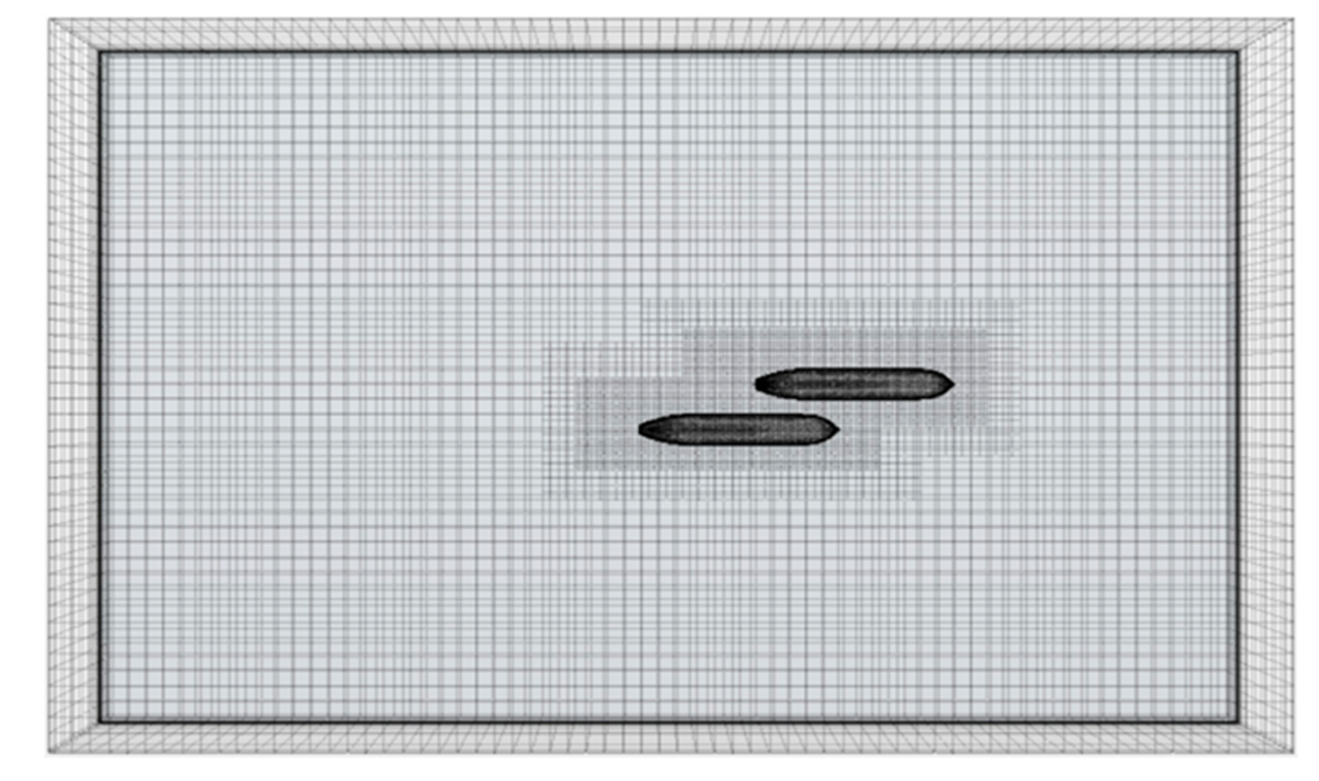
The dynamic simulation of the entire flow field is carried out in a rectangular parallelepiped. The height of the calculation domain is determined by the water depth. The length and the width of the calculation domain should be large enough for the full development of the propeller wake in the flow field. The boundary of the calculation domain is composed of the hull wall, velocity inlet, pressure outlet, non-slip bottom wall, two side planes, and the top boundary. The inlet is located at in front of the SOD ship, while the outlet is at behind it, and the two side planes are from the nearest sidewall of the ship. The free surface is from the top boundary and from the bottom wall, where is the depth-of-calculation condition. The rotating region containing the propeller is a cylinder that is in diameter and in height.
The spatial discretization of the entire calculation domain is composed of a trimmed mesh in a structured grid and polyhedral mesh solids in an unstructured grid. A structured mesh has the advantages of a simple data structure, high quality of grid generation, and fitting suitable for region boundaries, while an unstructured mesh can fully fill the calculated region and is often used for discretization of complex structures and surfaces. According to the geometric characteristics of the hull and propeller, the rotating region is discretized by a polyhedral element, and the other regions are discretized by trimmed elements, as shown in
Figure 3 and
Figure 4. In addition, local mesh refinement is carried out for the free surface, hull, rotating region, and near the rudder. It can be seen from
Figure 3 that the grid size increases successively from inside to outside with a growth rate of 2. Incremental distribution of grid size facilitates the formation of high-quality grid models and improves the convergence of calculations.
3.4. Convergence Study and Validation
Before the numerical simulations, a grid convergence analysis was carried out for the KVLCC2 hull model. The overlapping grid technique was used in the modeling of hull. The accuracy and convergence of the calculation are affected by the grid quality. Therefore, the sinkage of bare hull was calculated using three models of different meshes: coarse grid (M1), medium grid (M2), and fine grid (M3). The only variable was the grid base size, while the selection of physical model and discretization method were the same. The number of elements in the entire calculation domain was 0.86 × 10⁶, 1.35 × 10⁶, and 2.13 × 10⁶, respectively.
The speed of the hull is presented using the Froude number.
Figure 5 shows the numerical results for the hull sinkage obtained with three meshes at different Froude numbers, where the depth-to-draft ratio is 2. As shown in the figure, the results of the three grid calculation models fit well with the test results. The convergence factor
is used to represent the grid convergence of the numerical simulation, where
. When
, the results are monotonically convergent, and
is obtained from the numerical results. By comparing the test values, the average errors of the M1, M2, and M3 models were 2.1%, 1.9%, and 1.2%, respectively. Considering the calculation accuracy and efficiency comprehensively, the M2 grid model was used for the simulations of the hydrodynamic interaction.
Different turbulence models deal with the Reynolds stress term differently, resulting in different hydrodynamic values. Based on the same physical model and grid settings, the influence of different turbulence models (Realizable k−ε and SST k−ω) on the numerical results of propeller open water simulation was explored. The calculation domain consists of two cylinders. The rotating region is a small cylinder containing the propeller, and the stationary region is a large cylinder outside. The rotation region is discretized into polyhedral elements, and the static region is discretized by trimmed meshes.
The expected velocity coefficient
is obtained by changing the incoming flow velocity at the boundary of the computational domain when the propeller speed
is fixed at 594 rpm. The numerical solutions of propeller thrust and torque with different
values were obtained. After the nondimensionalization, the open water thrust coefficient
, torque coefficient
, and open water efficiency
of the KP458 propeller are shown in
Figure 6, together with the test data from Japan’s National Maritime Research Institute [
21]. The results show that the propeller motion can be well simulated using the reference coordinate system method, and the numerical results obtained by the Realizable
k−
ε turbulence model are closer to the test data, with a maximum error of less than 10%. In the following numerical simulations, the Realizable
k−
ε turbulence model is used.
4. Results and Analysis
The hydrodynamic interaction forces acting on DS are analyzed when the ship’s side is exposed in SOD’s propeller wake. The characteristics of the propeller disturbance flow field were investigated for various parameters, such as speed of the propeller, water depth, lateral distance, and the longitudinal distance between ships.
For the purpose of better presentation, analysis, and discussion, the hydrodynamic forces, moments, and relative positions involved are nondimensionalized. The hydrodynamic forces and are nondimensionalized as and , where is the water density and the draught of the vessel. Since the ship is stationary, the variable is the propeller speed , and the linear velocity , where is the diameter of propeller.
The nondimensional longitudinal distance is defined as . That is, when the two vessels are aligned at midship; when the aft perpendicular of ship SOD is aligned with the fore perpendicular of ship DS. The nondimensional lateral distance is defined as , where is the ship beam.
The influence of the propeller on the velocity field and pressure field in the computational domain is mainly significant in the wake area. Therefore, the relative longitudinal position
of the two ships was explored for the range of 0 to 3.2, namely, 0, 0.4, 0.8, 1.2, 1.6, 2.0, 2.4. 2.8, and 3.2. Other parameters analyzed are the lateral distance
, depth-to-draft ratio
, and propeller speed
. The cases of numerical simulations are given in
Table 2.
4.1. Interaction Forces and Moment in Case 1
The changes of the surrounding flow field caused by the propeller rotation of two KVLCC2 models at different longitudinal positions were simulated for the case of zero ship speed and zero incoming flow velocity.
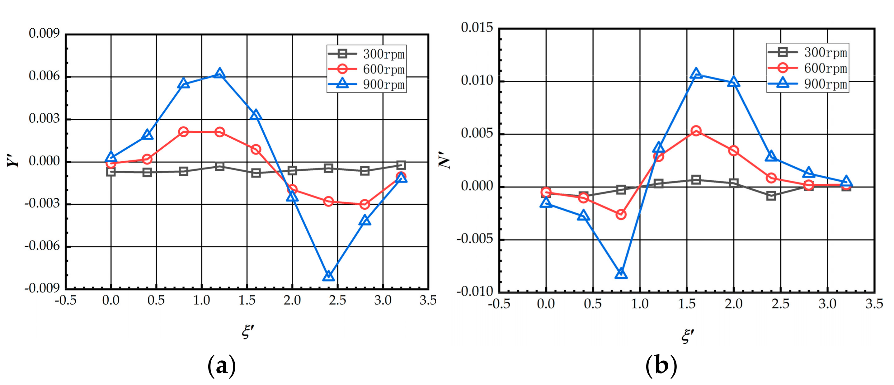
Figure 7 shows the lateral force
and yaw moment
obtained for the range of longitudinal relative positions between SOD and DS.
The hydrodynamic force and moment acting on SOD are obviously smaller than DS, and vary slightly with . When , i.e., when DS is located at a distance behind SOD, no significant variations of the hydrodynamic force and moment acting on SOD are observed. For DS, part of the hull is exposed to the wake of the propeller, and the flow of the surrounding fluid changes the surface forces on the hull, which is analyzed in detail next.
The hydrodynamic lateral force of DS can be divided into four stages according to . When , the lateral force is positive and monotonically increasing, which shows that the two ships are attracting each other. When , the lateral force decreases, which means that the two ships are being attracted to each other and the attraction force decreases as increases. When , the lateral force becomes a repulsion force and increases with , which shows that the ships repel each other and the repulsion force increases. When , DS is located relatively far behind the stern of SOD, the lateral force decreases, and the repulsion force decreases gradually as increases. There are four points of interest in the curve. The two peaks in interaction lateral force occur near and . When is approximately equal to 2.0, the interaction lateral force is zero. When reaches 3.2, the hydrodynamic interaction can be considered insignificant.
The variation in the hydrodynamic yaw moment acting on DS can be divided into five stages according to , namely, ,,,, and .
When , the yaw moment is negative and monotonically decreasing, which shows that the stern suction is acting on DS. When , the yaw moment increases and the stern suction effect decreases as increases. When , the yaw moment is positive and increasing, which is a bow suction. When , the yaw moment decreases rapidly as increases, i.e., the bow suction effect on DS decreases. When , the longitudinal distance between the two ships is somewhat large, the yaw moment continues to decreases, and the bow suction on DS gradually vanishes. The peak yaw moment acting on DS was observed at , and zero yaw moment was observed at .
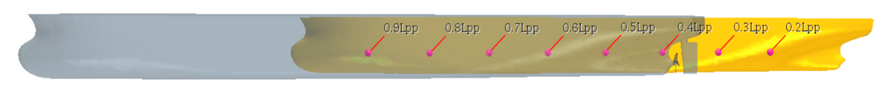
To investigate the pressure changes due to the propeller rotation, the pressure on the eight measuring points which were placed over the hull of DS were calculated in the numerical simulation. The position of the eight measuring points are shown in
Figure 8, and these measuring points were
below the waterline and evenly distributed between 0.2–0.9
Lpp with a spacing of 0.1
Lpp.
.
The pressure field around DS’s hull was changed due to propeller rotation.
Figure 9 and
Figure 10 show the hydrodynamic pressure at the pressure-measuring points at different values of
. In
Figure 9, the abscissas are the locations of the measuring points from the bow to the stern, and each curve shows the variation of pressure distribution along the ship hull, while
Figure 10 shows how the pressure at each point varies as the relative position changes, which corresponds to the pressure variation over time in the case of one ship overtaking another.
The hydrodynamic pressure changes obviously in the range of
.The local high-pressure and negative-pressure areas move forward as
increases, as shown in
Figure 9 where the four peaks appear at different locations in the direction of the ship length (
x/
Lpp) as
changes. The hydrodynamic pressure in the far front of the propeller is negative, and it is most obvious when
, while the pressure behind the propeller is positive. It can be seen that, when
, i.e., when the bow of DS is completely exposed in the propeller wake of SOD, the dynamic pressure is positive.
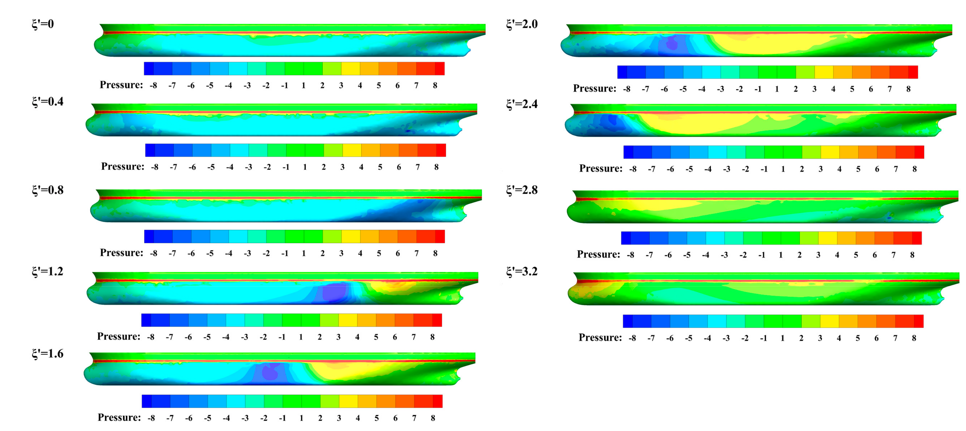
Taking
as an example, the dynamic pressure at the measuring points is represented by the blue line in
Figure 9, and the abscissa indicates the location of the measuring point illustrated in
Figure 8, where the SOD hull, together with its propeller and rudder, is depicted in transparent gray. The local high-pressure area is located in the wake area, but in front of the propeller and near the 0.5
Lpp measuring point instead. The dynamic pressure changes from positive at 0.5
Lpp to negative at 0.6
Lpp, and remains almost the same between 0.6 and 0.9
Lpp.
4.2. Free-Surface Elevation in Case 1
To further explore the propeller effect on the hydrodynamic interaction between ships, the free-surface elevation around the two ships due to the propeller motion was simulated. The free-surface elevation around the two ships at different longitudinal distances is shown in
Figure 11.
In
Figure 11a–c, it can be seen that, for small longitudinal distances, the propeller rotation creates significant surface elevations between the hulls. In comparison, for large relative distances between the ships, a majority of the ship hull of DS is exposed in the propeller wake, in which case the most significant surface elevation observed is on the left side of the DS, while the surface elevation on both sides of SOD and on the right side of DS is insignificant, as shown in
Figure 11d–i.
4.3. Pressure on the Hull Surface in Case 1
In order to correctly understand the characteristics of the hydrodynamic interaction force and moment, the surface pressure distribution of SOD and DS were investigated. According to the interaction caused by propeller rotation on the free surface, it can be found that the change in the flow field was significant mainly between SOD and DS. Therefore, the left side of the DS hull and the right side of the SOD hull are analyzed and presented here.
Figure 12 and
Figure 13 shows the dynamic pressure distribution on the hull surface of DS and SOD when the lateral distance is
.
Due to the suction effect of the propeller, a negative pressure zone occurs at the rear and right of the SOD. Affected by the propeller wake, the side pressure of the rudder is negative. By comparing the hull surface pressure at different
in
Figure 13, it can be found that the change in pressure with
is not significant, which is consistent with the variation pattern in the hydrodynamic force and moment acting on SOD. However, the surface pressure of DS changes significantly with the increase in
, so the results of the following analysis is mainly aimed at DS.
When
increases from 0 to 0.8, the pressure on the aft hull of DS decreases significantly, and a negative pressure zone is formed. When
, the negative pressure moves towards to the bow of DS as
increases from 0.8 to 2.4. The location of the low-pressure area on the side of the DS hull is consistent with the trough of the surface elevation, as shown in
Figure 11.
A high-pressure zone, right after the negative-pressure zone, is also formed when
, and this high-pressure zone moves together with the negative-pressure zone towards the bow as
increases. When
, the maximum pressure in this zone reaches its maximum and then declines. This phenomenon matches well with the surface elevation around the hull of DS as shown in
Figure 11.
At
=2.8, the negative-pressure zone disappears and the high-pressure zone continues to moves to the very rear end of the hull of DS, as shown in
Figure 12.
The rotation of the propeller drives the flow of water, which changes the velocity field of the fluid around the hull. The uneven velocity distribution around the DS hull leads to the difference in the surface pressure. The uneven distribution of force on the hull surface is the cause of hydrodynamic force and moment, showing the behavior of suction and repulsion forces. When
, the hull on the left side of DS under the water line is under negative pressure, so the lateral force is positive, indicating that the two ships are attracted to each other. When
, the decrease in pressure on the aft body of the hull is most significant, which contributes to a large negative moment acting on the hull that is manifested as stern suction. When
, a high-pressure zone appears after the negative-pressure zone, and the stern suction phenomenon is weakened due to the cancellation effect of the high-pressure zone. As the low-pressure area moves forward, the stern suction becomes bow suction. In conclusion, the variation of DS side pressure distribution is coupled with the variation pattern of hydrodynamic force and moment shown in
Figure 7.
4.4. Influencing Factors
4.4.1. Propeller Speed
To investigate the effect of propeller speed on the hydrodynamic forces, the simulations of Case 2 shown in
Table 2 were carried out.
Figure 14 shows how the hydrodynamic lateral force
and yaw moment
acting on the DS vary with
at different propeller speeds. The peak hydrodynamic force and moment increase with the propeller speed. At low speed (
), a negative sway force, i.e., a repulsion lateral force, acting on DS is produced, and the lateral force does not change significantly with the longitudinal distance between the two ships. As the propeller speed increases to 600 rpm and 900 rpm, a significant increase in the magnitude of the hydrodynamic force and moment acting on DS is observed. However, unlike the case of
n = 300 rpm, the sign of the lateral force depends on the relative position of the two ships; a positive peak of lateral forces appears at
, and a negative peak appears at
. For the moment acting on DS, a similar change in magnitude is also observed; however, a negative peak appears at 0.8 and a positive peak at
.The thrust
and torque
of the KP458 propeller with speed
and velocity coefficient
in open water [
19] is used to quantify the propeller-induced interaction forces; when the propeller speed is 900 rpm, the maximum lateral force acting on DS is about
and the maximum yaw moment is about
.
Figure 15 shows the pressure distribution on the hull surface at the corresponding longitudinal distance at different propeller speeds. When the propeller speed is 300 rpm, there is no significant pressure change on the hull of DS, and this observation is consistent with the relatively small hydrodynamic interaction forces, as shown in
Figure 14. For the cases of 600 rpm and 900 rpm, significant changes in pressure on the hull are observed, and consistency can also be found with the hydrodynamic forces acting on DS.
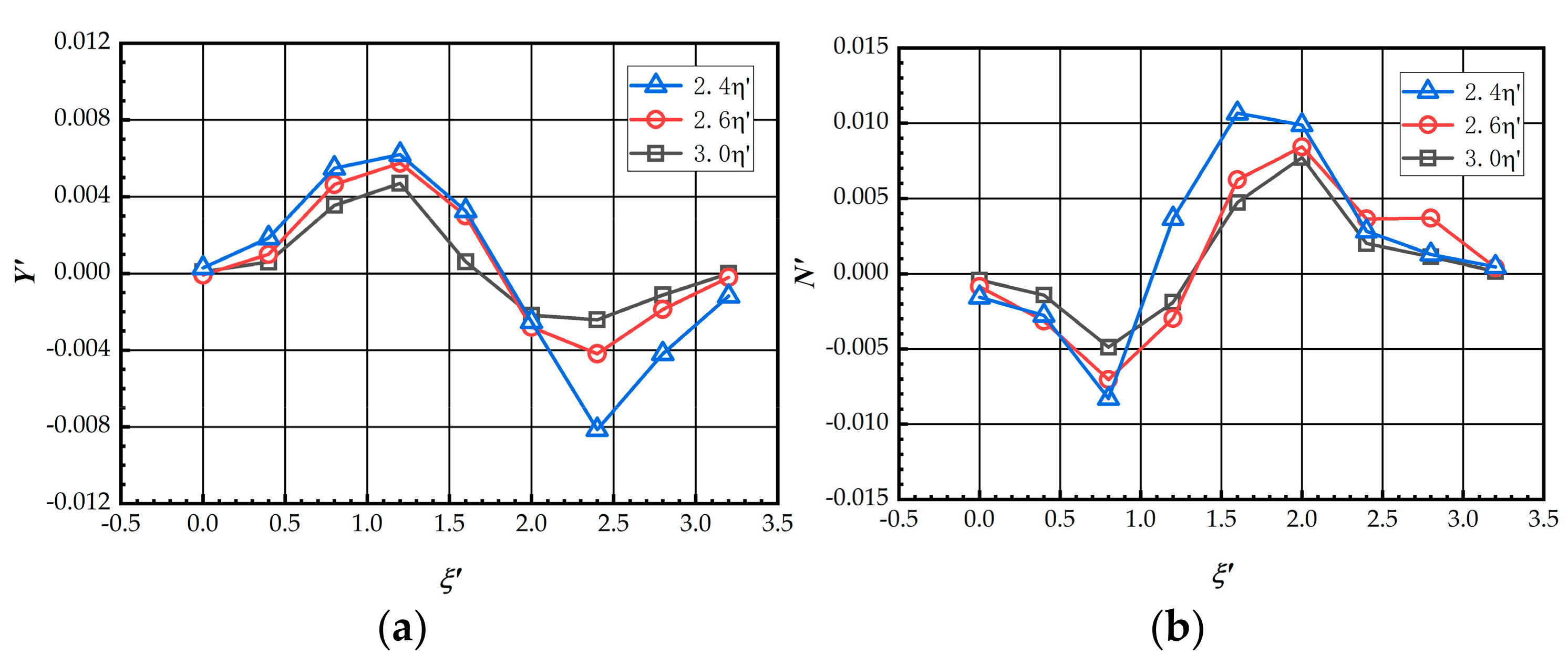
4.4.2. Ratio of Depth to Draft
To investigate the influence of water depth, a group of simulations was carried out with various water depths, i.e., Case 3 in
Table 2. It can be seen that the water depth has a great influence on the sway force and yaw moment acting on DS.
It can be seen in
Figure 16b that, as the depth-to-draft ratio decreases from 3 to 2, the peak yaw moment is increased by 70%, and, as the depth-to-draft ratio decreases from 2 to 1.5, peak yaw moment increases by 42%. For the sway force, the change in the peak force is relatively small when the ratio decreases from 3 to 2, but significant when the ratio decreases from 2 to 1.5. When the depth-to-draft ratio is 1.5, the maximum lateral force acting on DS is about
and the maximum yaw moment is about
.
The patterns shown in
Figure 16 are consistent with the changes in pressure distribution on the hull shown in
Figure 17. In the case of
, a decrease in depth leads to the decrease in pressure in the negative-pressure zone at the stern of DS and results in an increase in the sway force. Since there is little change in the pressure in the front of the hull as the water depth decreases, such a decrease in the pressure at the stern results in greater yaw moments.
In the case of , with the decrease in depth, the negative-pressure zone moves forward and the positive-pressure zone expands in area, which intensifies the bow attraction and stern repulsion of DS.
4.4.3. Lateral Distance
To investigate the effect of lateral distance on the hydrodynamic forces, the simulations of Case 4 shown in
Table 2 were carried out.
Figure 18 shows how the hydrodynamic lateral force
and yaw moment
acting on the DS vary with
at different lateral distances.
It can be seen that the peak hydrodynamic force and moment increase as the lateral distance decreases. The peak lateral force increases by 73% as the lateral distance decreases from
to
, and it increases by 94% as the lateral distance decreases from
to
. For the yaw moment acting on DS, as shown in
Figure 18b, a clear pattern is observed; that is, the yaw moment increases with the decrease in lateral distance, and the effect of lateral distance is most significant when the lateral distance reduces from
to
. Since it is indicated in
Figure 18 that the peak yaw moment appears at
and
, the pressure distributions on the hull surface at these two relative locations are extracted and presented in
Figure 19, where the pressure distributions are compared for the three different lateral distances. The two distributions presented in each row correspond to the two cases of the same lateral distance but at the negative and positive peak yaw moment, while the distributions in each column correspond to the negative peak yaw moment at different lateral distances. By a closer inspection of the left column and the right column, it can be found that a negative-pressure zone is located at the stern in each distribution in the left column, and, in contrast, in the distributions in the right column, a negative-pressure zone is present at midship and a positive-pressure zone appears at the stern. The observation indicates that the peak yaw moment induced by the propeller effect mostly appears at a certain longitudinal distance between the two ships, while the lateral distance only has an effect on the magnitude.


