Coupled Vibration Analysis of Ice–Wind–Vehicle–Bridge Interaction System

Abstract

Bridges built in ice-covered water regions are mostly in complex marine environments, they not only need to withstand strong wind but also resist the impact of drift ice. However, at present, there is a lack of vehicle–bridge coupling vibration analysis and driving safety assessment under combined ice and wind. Therefore, this study constructs a complete analysis framework of ice–wind–vehicle–bridge interaction to investigate the dynamic responses of the coupled system. Ice load is simulated by a linearized ice–structure interaction model, which is based on the self-excited vibration theory. Wind load on the bridge deck includes steady-state force and buffeting force. Wind load on the vehicle is simulated based on the quasi-steady model. Subsequently, ice load, wind load, soil–structure interaction (SSI), and additional water mass are all integrated into a full bridge model based on a sea-crossing bridge with running vehicles in the Bohai Sea. The results indicate that ice load has a greater impact on the lateral dynamic response of the bridge, the combined action of ice and wind has no superimposed effect on the movement of the bridge but has a restraining effect. Wind load presents a more significant influence on the lateral dynamic response of the vehicle, the coupled dynamic responses of the vehicle cannot be combined by the superposition under separate ice and wind. The combined effect of ice and wind obviously increases the sideslip risk of running vehicles and reduces driving safety.

1. Introduction

There is a harsh working environment for sea-crossing bridges in cold sea regions. As well as being able to withstand the impact of ice load, it must also take into account the combined effect of strong wind, water–structure interaction, soft foundation on the seabed, and other complex factors. This poses a threat to the safety of bridges. Therefore, the coupled vibration analysis of ice–wind–vehicle–bridge interaction system is an unavoidable research topic for the construction of bridges in cold sea regions.

As bridge spans and vehicle axle weights increase on highway bridges, vehicle–bridge interactions have become more prevalent. The theory of vehicle–bridge interaction has evolved since the 1970s, with the advent of the finite element method and the application of computers in civil engineering. Vehicle–bridge interaction models have evolved to include complex vehicle models, bridge models, and pavement roughness models. A variety of models have been developed to study the vibration response of interacting systems in the development of vehicle–bridge coupling research. Yang and Lin [1] solved the integral equation of the vehicle–bridge interaction system by using the structural dynamic reduction measure to lower the vehicle freedom. It is an effective method for calculating the bridge response, but it is not sufficient to calculate the vehicle response. A method for calculating vehicle–bridge coupling was developed by Neves et al. [2]. In this study, the vehicle and bridge control equations were complemented by additional constraint equations, which realized the coupling of the vehicle contact node displacements with the corresponding node displacements of the bridge. Lu et al. [3] based on penalty functions built in ABAQUS software to define the vehicle–bridge contact conditions and realize the simulation of vehicle–bridge interactions. Additionally, the numerical results agree well with the analytic solution of the classic vehicle–bridge contact behavior proposed by Yang and Yau [4], which proves the correctness of the proposed method.

Many scholars have carried out targeted studies on the analysis of vehicle–bridge coupled vibration under different influence factors. For pavement smoothness, Camara et al. [5] proposed a wind–vehicle–bridge coupling analysis framework considering the random characteristics of bridge deck roughness and further conducted a risk analysis of driving safety subjected to wind load. Xie et al. [6] established a stochastic vehicle–bridge coupling model. It used the pavement spectrum to simulate the conversion of pavement unevenness and introduced the probability density evolution method. For seismic action, Li et al. [7] investigated the dynamic response of the vehicle–bridge interaction system of a continuous steel bridge with high piers under seismic action and examines how vehicle and bridge dynamics are affected by parameters such as ground shaking, PGA value, and pier height. Wang et al. [8] established a numerical simulation platform for seismic–wind–vehicle–bridge coupled vibration analysis and investigated the effect of complete spatial variability of ground shaking on the dynamic response of the coupled seismic–wind–vehicle–bridge system. Paraskeva et al. [9] established a framework for the coupled dynamic analysis of vertical seismic excitation off-vehicle-bridge, by which the influence of the roughness of the bridge deck on the dynamic response of the vertical seismic excitation off-vehicle-bridge system was focused on. For the wind load, Zhou et al. [10] accurately acquired vehicle response considering the interaction influence between vehicle flow, bridges, and wind loads. Xu and Guo [11] constructed a coupled dynamic analysis framework for vehicles and cable-stayed bridges under turbulent wind effects and investigated the vibration response of the vehicle–bridge system. Han et al. [12] explored the influence of the aerodynamic parameters on the vibration response of the vehicle–bridge system. Guo and Xu [13] investigated the safety of large-span bridges under crosswind action as well as the critical vehicle velocities for accidents like sideslips and rollovers. For the ice load action, Xia [14] established a numerical analysis model of the vehicle–bridge coupled system under ice load and proposed an iterative method applicable to the time-integrated full process of the vehicle–bridge dynamic coupled system. Xia et al. [15] systematically investigated the influence law of impact load type, impact intensity, and train velocity on the safety index. Specifically, they described the method for determining the impact intensity-train velocity threshold curve. Wu et al. [16] defined the contact relationship between the wheels and the bridge deck by using the penalty function method and analyzed the driving safety under the random vibration caused by ice load.

In summary, many studies have been conducted in the analysis of vibration between vehicles and bridges. However, there is a lack of research on the vibration between vehicles and bridges under the combined action of ice and wind. This study systematically studies the vibration of bridges and vehicles under ice and wind loads and analyzes the effects of different ice and wind velocities on the safety of traffic on bridges. The schematic of the simulation process for ice–wind–vehicle–bridge interaction is shown in Figure 1.

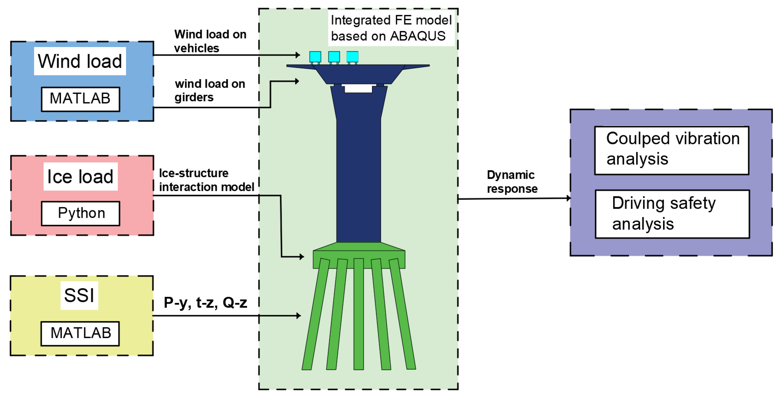
2. Analysis Framework of Ice–Wind–Vehicle–Bridge Interaction System

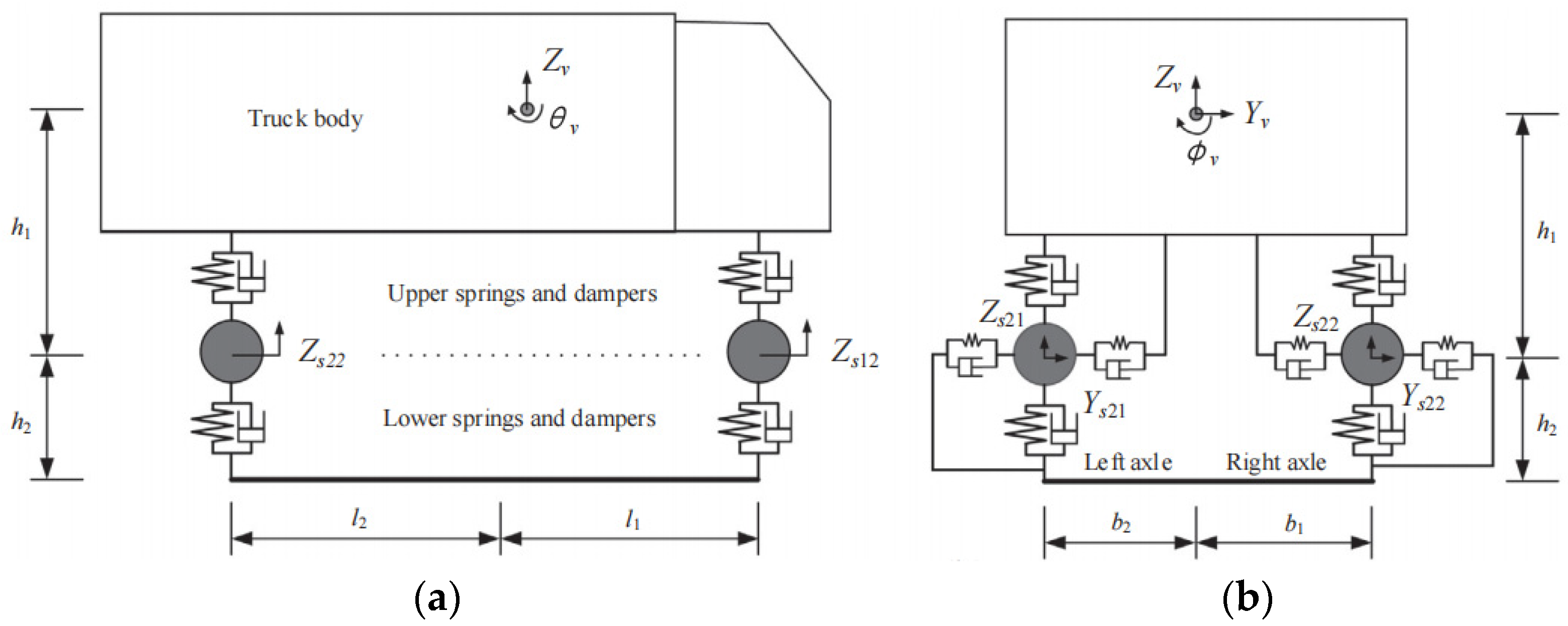
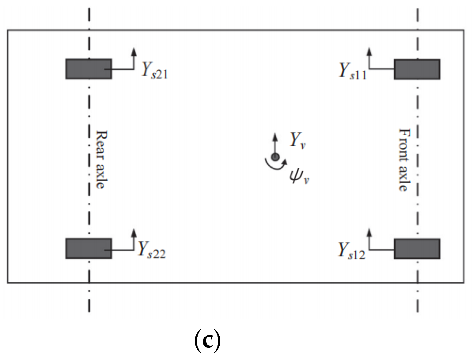
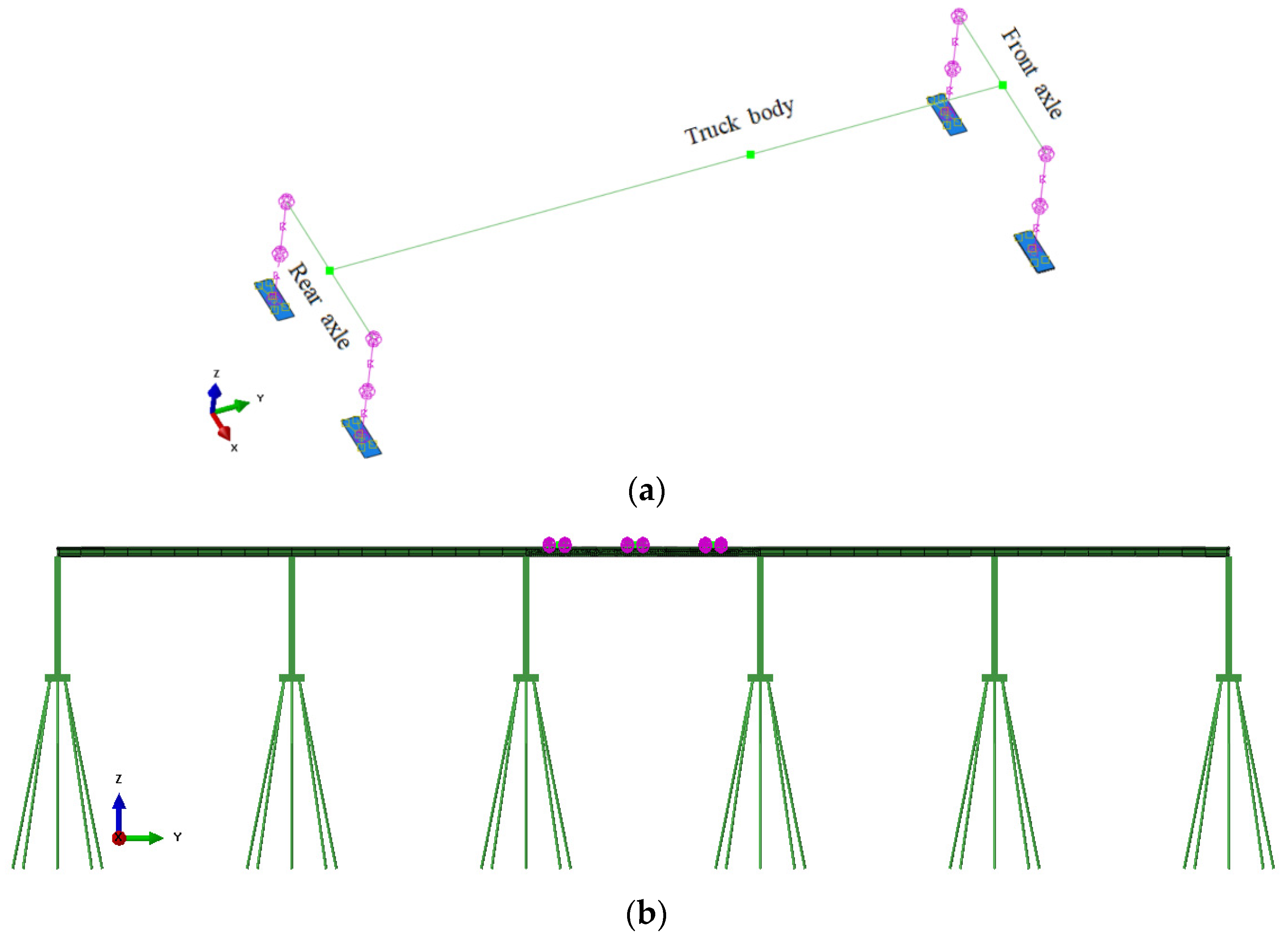
2.1. Modeling of the High-Sided Road Truck

Due to the typical accident-prone characteristics of the high-sided road truck compared with other types of vehicles [11,16,17], this study focuses on the vehicle–bridge interaction and driving safety of the high-sided road truck under lateral load. A two-axle four-wheel light high-sided road truck was adopted in this study, as shown in Figure 2. The light truck was composed of rigid body, spring, and damper, with 13 DOF. The following generalized motion vector can represent the dynamical system of the light truck used in this study.

$$V=\left\{Z_v Y_v {\theta }_v {\phi }_v {\psi }_v Z_{s11} Y_{s11} Z_{s12} Y_{s12} Z_{s21} Y_{s21} Z_{s22} Y_{s22}\right\}$$

(1)

where Z_v is the vertical displacement of the vehicle, Y_v is the lateral displacement of the vehicle, θ_v denotes the pitch angle of the vehicle, φ_v denotes the rotation angle of the vehicle, ψ_v represents swing angle of the vehicle. Z_s11, Z_s12, Y_s11, and Y_s12, respectively, represent the vertical displacement and lateral displacement of the two rigid bodies on the front axle of the vehicle. Z_s21, Z_s22, Y_s21, and Y_s22, respectively, represent the vertical displacement and lateral displacement of the two rigid bodies on the rear axle of the vehicle body.

Each rigid body in the front and rear axles of the vehicle was connected to the vehicle body through suspension units, including vertical linear elastic springs K_uzi and viscous dampers C_uzi, and horizontal linear elastic springs K_uyi and viscous dampers C_uyi. In addition, each rigid body in the front and rear axles of the vehicle was connected to the bridge deck through tire units, including vertical linear elastic springs K_lzi and viscous dampers C_lzi, and horizontal linear elastic springs K_lyi and viscous dampers C_lyi. The detailed parameters of the high-sided truck can be found in [11].

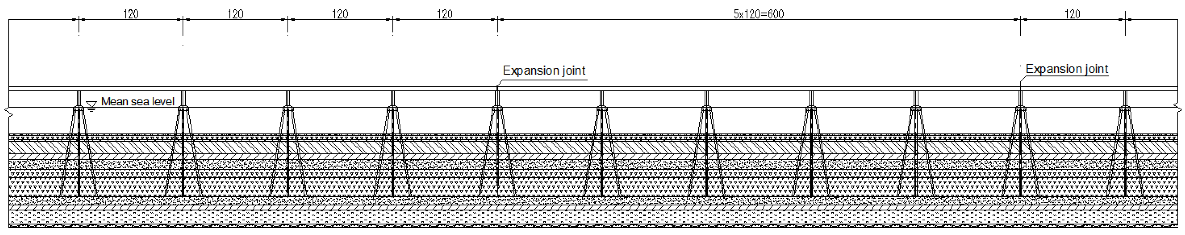
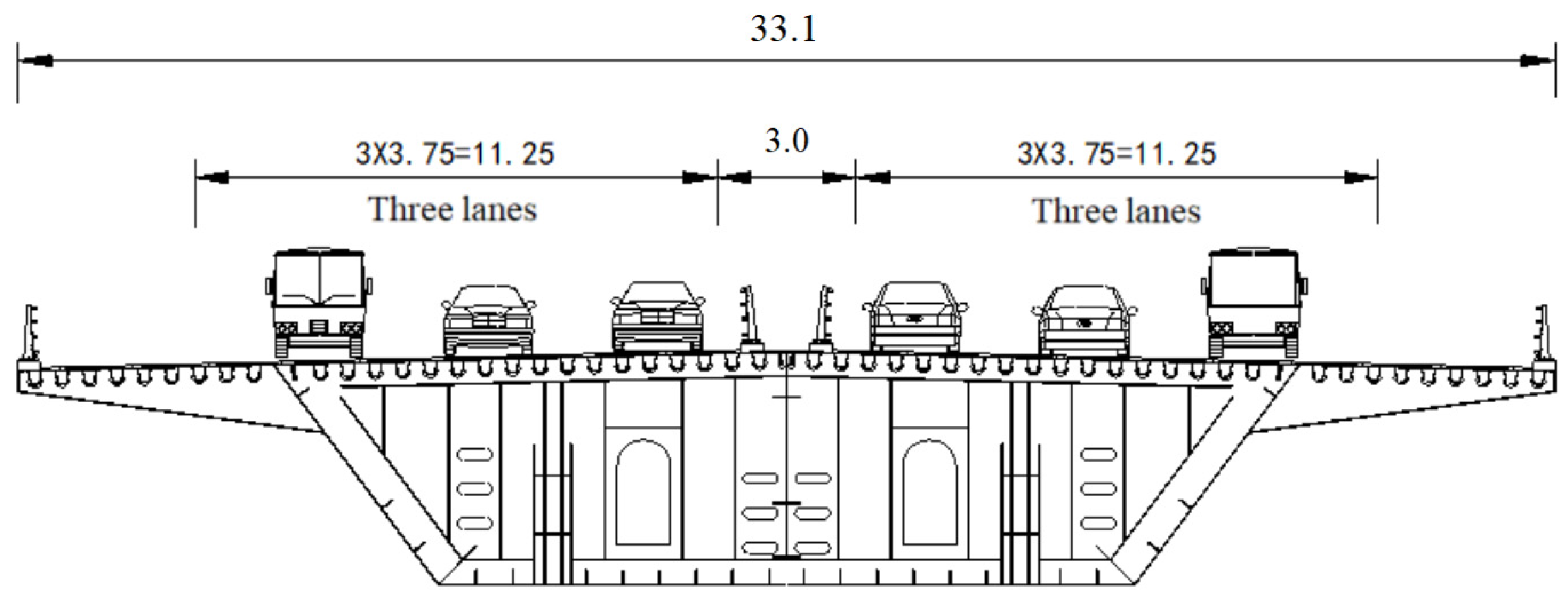
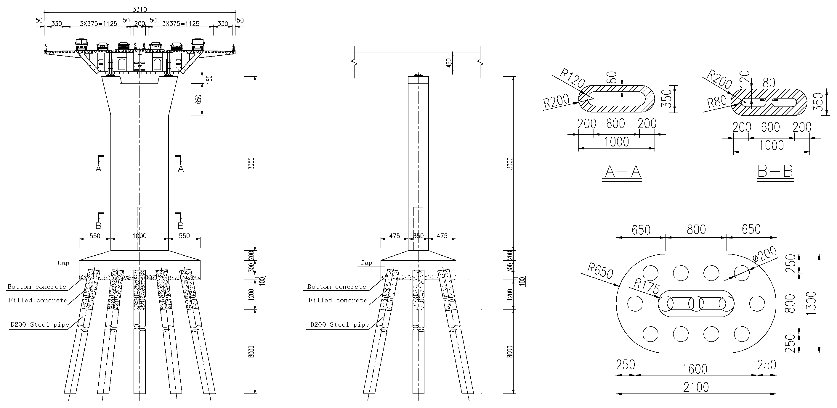
2.2. Modeling of the Sea-Crossing Bridge

The bridge construction conditions in the Bohai Sea are different from those in other sea areas. The difference is that bridges in the Bohai Sea are affected by winter ice floes every year. In this study, the non-navigable span of the sea-crossing bridge in the Bohai Sea was selected as the research object. The overall configuration of (5 × 120) m non-navigable bridge is shown in Figure 3. The cross-section form of the bridge girder is a steel box girder section, and two-way 6 lanes are set, as shown in Figure 4. The pier is of round end hollow section, and the material is reinforced concrete. The structural form of a high pile-cap foundation is adopted in the design of the bridge. The pile cap is 6 m high, and the plane size is 13 × 21 m. The pile foundation is supported by steel pipe piles. The specific size of the bridge substructure can be seen in Figure 5. In bridge design, the pile cap is located at the design water level elevation, so drift ice can affect the large volume of the pile cap, rather than acting on the pier or pile foundation.

The overall bridge model was established based on ABAQUS finite element platform. The girder of the bridge was built by the spatial plate element (S8R). The piers, pile caps, and steel pipe piles were modeled by the beam element (B31). The calculation methods for additional water mass and nonlinear soil spring can be found in previously published studies [18,19,20,21]. The dynamic action of water was simulated by the additional water mass. In the current work, the water depth of 30 m was selected to represent the typical deep-water state. The soil–structure interaction (SSI) was considered by using the classical p-y nonlinear soil spring. In this study, the typical soft clay geological condition was considered. Figure 6 shows the p-y, t-z, and Q-z curves with undrained shear strength Su = 25 kPa.

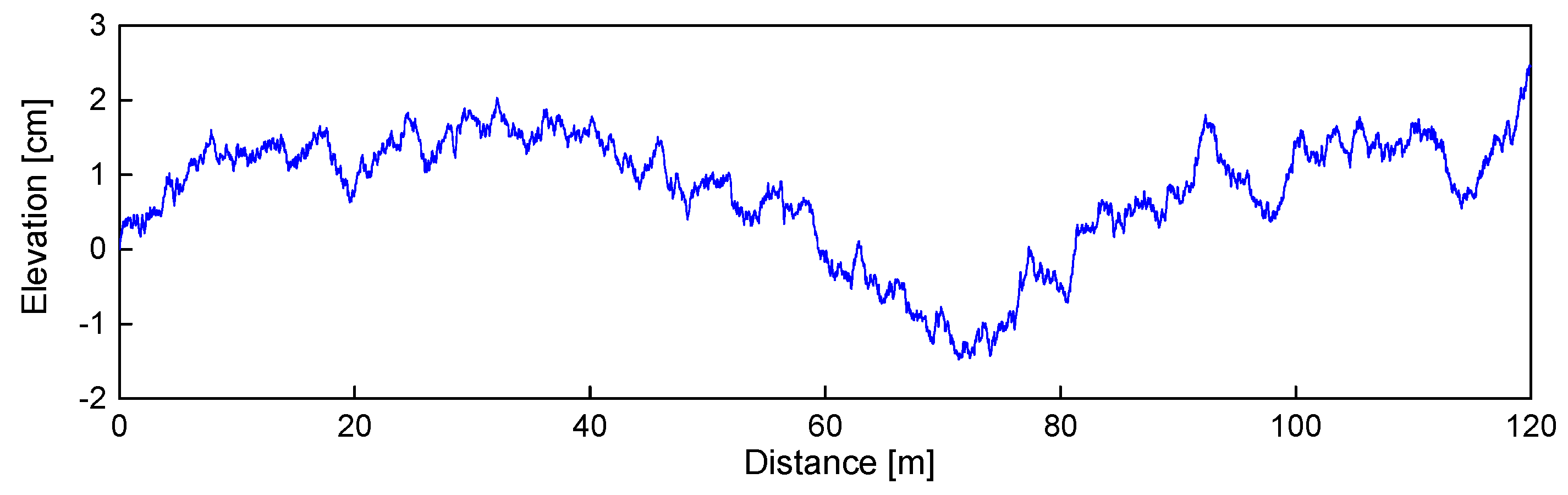
2.3. Modeling of Pavement Roughness

In the criterion ISO-8608 [22], a PSD function is given to describe the simulation of pavement roughness. This function can be expressed as [22,23]:

$$\phi \left(n\right)=\phi \left(n_0\right) {\left(\frac{n}{n_0}\right)}^{-2}$$

(2)

in which n is the spatial frequency, n₀ denotes the reference frequency, φ(n₀) denotes the pavement irregularity coefficient.

The function r(x) of pavement roughness can be given as follows [23,24]:

$$r\left(x\right)={\displaystyle \sum _{k=1}^N\sqrt{2\phi \left(n_k\right)\Delta n}\cos \left(2\pi n_{k}x+{\theta }_k\right)}$$

(3)

here θ_k is phase angle, n stands for the wave number.

In this study, the pavement conditions with “good” grade of pavement irregularity given in the criterion ISO 8608 [22] were adopted. The simulated road irregularities are given in Figure 7.

It should be noted that the pavement irregularity is realized by changing the absolute altitude coordinate of corresponding nodes on the deck of bridges.

2.4. Modeling of the Vehicle-Bridge Contact Behavior

The penalty function method is a very common contact interface algorithm, which is widely used in numerical calculation. The basic principle of the penalty function is as follows: First, the penalty function is established by using the constraint property. Then, the penalty function is added to the objective function to transform it into an unconstrained problem. Thus, the solution of the new objective function is consistent with that of the original objective function. The objective function f(x) can be expressed as:

$$\left\{\begin{array}{c}\min f\left(x\right)\\ s.t.g_i\left(x\right)=0\end{array}\right.$$

(4)

here, f(x) is the objective function, g_i(x) is the constraint condition.

The augmented objective function can be expressed as:

$$\min F\left(x,\sigma \right)=f\left(x\right)+\sigma P\left(x\right)$$

(5)

here, $\sigma$ is the penalty factor, $F\left(x,\sigma \right)$ denotes the penalty function, $\sigma P\left(x\right)$ stands for the penalty term.

The specific principle of penalty function method is at each time step, first check whether each slave node penetrates the main surface, and if it does not penetrate, do not do any processing. In the case of penetration, a large interface contact force will be introduced between the slave node and the penetrated surface, and its magnitude is proportional to the penetration depth and the rigidity of the main surface. Many studies have proved that the contact problem defined by the penalty function can show results close to the actual problem [3,25,26]. For instance, Lu et al. [3] used the penalty function method to simulate the vehicle–bridge interaction and obtained analysis results consistent with the analytical solution.

In this study, the vehicle model, the bridge model, SSI, wind loads on vehicles and girders, ice loads on pile caps are integrated into ABAQUS software. The finite element model of vehicle–bridge coupling system is based on ABAQUS in this work, as shown in Figure 8. The contact condition between the wheel and the bridge deck is defined by the penalty function in ABAQUS software. The equation of motion is solved with the help of the implicit solver in ABAQUS software. In order to better explain the simulation process of the ice–wind–vehicle–bridge interaction system based on ABAQUS software, a solution flowchart is given in Figure 9.

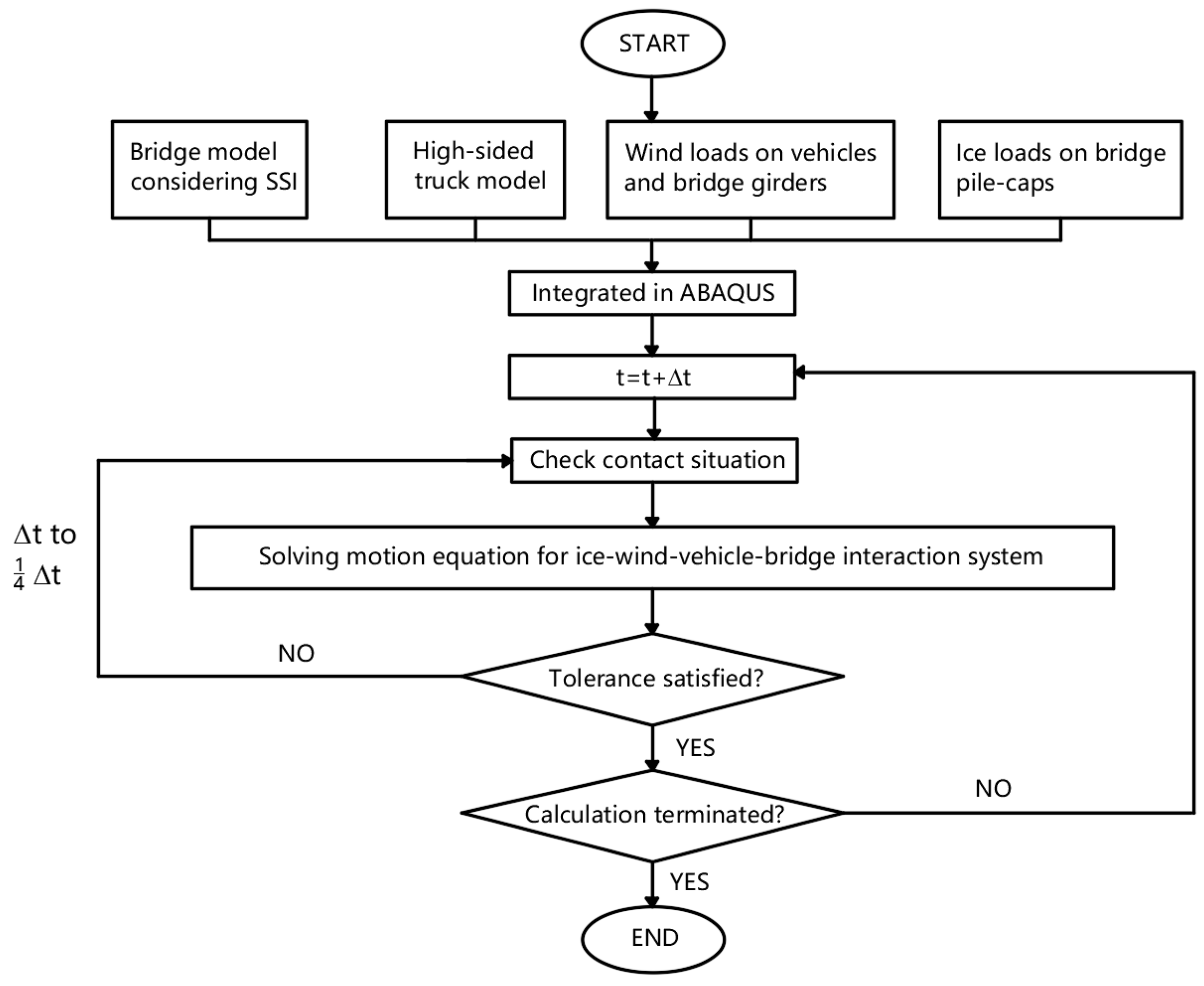
2.5. Coupled Dynamic Equation of Ice–Wind–Vehicle–Bridge Interaction System

The coupled dynamic equation was established with full consideration of vehicles, bridges, additional water mass, and soil–structure interaction. Ice load and wind load are applied to the overall dynamic system as external loads. Therefore, the coupled dynamic equation of the ice–wind–vehicle–bridge interaction system can be expressed as:

$$\left[\begin{array}{l}{M}_{bb}+M_w\hspace{1em}0\\ Sym\hspace{1em}\hspace{1em} M_v\end{array}\right]\left\{\begin{array}{l}{\ddot{w}}_b\\ {\ddot{w}}_v\end{array}\right\}+\left[\begin{array}{l}{C}_{bb}+C_i\hspace{1em}{C}_{bv}\\ Sym\hspace{1em}\hspace{1em} {\overline{C}}_v\end{array}\right]\left\{\begin{array}{l}{\dot{w}}_b\\ {\dot{w}}_v\end{array}\right\}+\left[\begin{array}{l}{K}_{bb}+K_s\hspace{1em}{K}_{bv}\\ Sym\hspace{1em}\hspace{1em} {\overline{K}}_v\end{array}\right]\left\{\begin{array}{l}{w}_b\\ w_v\end{array}\right\}=\left\{\begin{array}{l}{F}_{bb}+F_{ice}+F_{bw}\\ F_{vv}+F_{vw}\end{array}\right\}$$

(6)

here, subscripts bb denotes the bridge, vv denotes the vehicle, and bv denotes the vehicle–bridge interaction.

The overall mass matrix includes mass matrix M_bb of the bridge and additional water mass matrix M_w. The overall damping matrix includes damping matrix C_bb and the self-excited ice force additional damping matrix C_i. It should be noted that because there is an additional damping term C_i, the new damping term in the motion equation includes the damping of the bridge structure and the damping caused by ice load. The specific explanation is described in Section 3.1 below. The stiffness matrix includes vehicle–bridge coupling stiffness matrix K_bb and soil spring additional stiffness matrix K_s. M_v represents the mass matrix corresponding to all vehicle inertia forces.

In the ice–wind–vehicle–bridge interaction system, the dynamic response of the coupling system depends on the DOF of the vehicle, the DOF of the bridge, and the pavement irregularity. Therefore, the coupling damping matrices C_bv and C_vb and the coupling stiffness matrices K_bv and K_vb are used to construct the coupling vibration equations. The vehicle damping matrices of the overall interaction system ${\overline{C}}_v$ include additional damping matrix to the vehicle damping matrix C_v. Similarly, the vehicle stiffness matrices of the overall interaction system ${\overline{K}}_v$ also include an additional stiffness matrix. F_bb is composed of two parts: Vehicle body gravity and vehicle–bridge interaction force, depending on vehicle–bridge response. F_vv is also the vehicle–bridge interaction force that depends on dynamic response. F_ice denotes the overall ice load vector under ice-induced vibration. The F_bw is the total wind load vector on the bridge. F_vw is the overall wind load vector on the vehicle.

3. External Excitation Loads

3.1. Ice-Induced Vibration Model

3.1.1. Negative Damping Effect

For the problem of ice-induced vibration, Määttänen [27] proposed a self-excited vibration theory of ice-induced structures based on the nonlinear relationship between ice-crushing strength and strain rate. Combining the structural motion equation with crushing strength of ice, the phenomenon of self-excited vibration between ice and structure is explained by using negative damping. The system motion equation under ice-induced vibration can be described as

$$M\ddot{u}+C\dot{u}+Ku=F\left(v_r\right)=F\left(v_{ice}-\dot{u}\right)$$

(7)

where $v_r=v_{ice}-\dot{u}$ is the relative velocity, $F\left(v_{ice}-\dot{u}\right)$ represents the total ice force.

According to Equation (7), the terms of ice force on the right side of the equation are related to the structure velocity. Using the first-order Taylor expansion, the ice force term is transformed at the point $\dot{u}$= 0, and the following can be obtained:

$$F\left(v_r\right)=F\left(v_{ice}-\dot{u}\right)\approx F\left(v_{ice}\right)+\frac{dF\left(v_{ice}\right)}{d{v}_r}\left(-\dot{u}\right)$$

(8)

Therefore, the equation of motion of ice and structure interaction can be rewritten as:

$$M\ddot{u}+\left(C+\frac{dF\left(v_{ice}\right)}{d{v}_r}\right)\dot{u}+Ku=F\left(v_{ice}\right)$$

(9)

where $C+\frac{dF\left(v_{ice}\right)}{d{v}_r}$ is a new damping term in the structural system.

If the negative value $C+\frac{dF\left(v_{ice}\right)}{d{v}_r}$ obtained by the damping term is greater than the damping constant of the structure itself, then the whole system obtains negative damping. Negative damping leads to the instability of the dynamic system. However, due to the nonlinear relationship between ice-crushing strength and strain rate, its vibration amplitude cannot increase infinitely but can stabilize within a stable limit cyclic amplitude. This limit cycle indicates energy dissipation and external energy supply of the whole system in a vibration cycle are balanced [28].

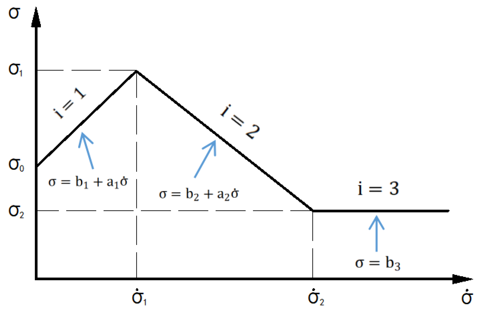
3.1.2. Linearized Model of Ice–Structure Interaction

It has been found that the ice-crushing strength is a function of the ice stress rate [29,30]. In other words, the compressive capacity of ice depends on the compression rate of ice. The compression crushing process of ice is divided into three regions: Ductile region, ductile-brittle transition region, and brittle region. When the ice falls in the ductile region, its compression strength increases with the increase in stress rate. In the ductile-brittle transition region, the ice-crushing strength reaches the maximum. In the brittle region, the crushing strength of ice decreases by about 50% to 70% from the maximum value [31]. The crushing strength of ice shows a decreasing trend, and finally, tends to be flat. In this study, the expression of ice compression strength and stress rate is piecewise linearized, as shown in Figure 10. After linearization, the multilinear relationship between ice compression strength and stress rate can be approximately expressed as:

$${\sigma }_i=b_i+a_i\dot{{\sigma }_i}$$

(10)

where a_i and b_i are the slope and intercept of segment i. σ_i is the ice-crushing strength. Among them, σ₁ is the maximum crushing strength in the ductile-brittle transition region, σ₀ is the initial crushing strength in the ductile failure region, which is usually taken as 2/3 of σ₁. σ₂ is the crushing strength of ice in the brittle failure region, which is usually taken as 1/3 of σ₁. $\dot{{\sigma }_i}$ is the stress rate of ice. Among them, the stress rates corresponding to the maximum crushing strength of ice in the ductile-brittle transition region and brittle failure region are taken as $\dot{{\sigma }_1}=0.3$ MPa/s and $\dot{{\sigma }_2}=1.3$ MPa/s. For $\dot{\sigma }<0.3$ MPa/s, the crushing strength of ice increases with the increase in stress rate. When the stress rate is in the range of $0.3<\dot{\sigma }<1.3$ MPa/s, the crushing strength of ice decreases with the increase in stress rate. When the stress rate exceeds 1.3 MPa/s, the crushing strength of ice remains unchanged and is a constant value.

Määttänen [27] gives the expression of stress rate and relative velocity during the compressive failure of ice.

$$\dot{{\sigma }_i}=8{\sigma }_1{v}_r/\pi D$$

(11)

where D is the structure diameter.

Therefore, the total ice force on the structure can be written as:

$$\begin{gathered} F\left(v_r\right)=F\left(v_{ice}-\dot{u}\right)=A\times \sigma \left(v_{ice}-\dot{u}\right)=A\left(a_i\times \left(v_{ice}-\dot{u}\right)\frac{8{\sigma }_1}{\pi D}+b_i\right) \\ =\left(A\times b_i+v_{ice}\times A\times a_i\frac{8{\sigma }_1}{\pi D}\right)-\dot{u}\times A\times a_i\frac{8{\sigma }_1}{\pi D} \end{gathered}$$

(12)

where h is the ice thickness, A is the contact area under ice-induced vibration.

Among them, the ice force part only related to ice velocity can be expressed as:

$$F\left(v_{ice}\right)=\left(b_i+v_{ice}\times a_i\frac{8{\sigma }_1}{\pi D}\right)$$

(13)

The new damping coefficient in the structural system can be expressed as:

$$C_{new}=C+a_i\frac{8{\sigma }_1}{\pi D}A$$

(14)

For the linearized ice load model, the ice load simulation can be divided into three piecewise functions according to the ice stress rate, which can be written as:

$$F\left(v_{ice}\right)=\left\{\begin{array}{c}\left(b_1+v_{ice}\times a_1\frac{8{\sigma }_1}{\pi D}\right)A \dot{\sigma }<\dot{{\sigma }_1}\\ \left(b_2+v_{ice}\times a_2\frac{8{\sigma }_1}{\pi D}\right)A \dot{{\sigma }_1}<\dot{\sigma }<\dot{{\sigma }_2}\\ b_{3}A \dot{\sigma }>\dot{{\sigma }_2}\end{array}\right.$$

(15)

The damping coefficient changes with the stress rate of ice, and its subsection expression can be written as:

$$C^{\prime }=\left\{\begin{array}{c}{a}_1\frac{8{\sigma }_1}{\pi D}A \dot{\sigma }<\dot{{\sigma }_1}\\ a_2\frac{8{\sigma }_1}{\pi D}A \dot{{\sigma }_1}<\dot{\sigma }<\dot{{\sigma }_2}\\ 0 \dot{\sigma }>\dot{{\sigma }_2}\end{array}\right.$$

(16)

It should be noted that this study is based on the secondary development interface of the ABAQUS finite element platform and uses FORTRAN language to develop user subprograms. The individual user programming of the ice-induced vibration model is applied to ABAQUS software, thus realizing the interaction analysis of ice and bridge.

3.2. Wind Load

3.2.1. Wind Load on Bridges

The wind load on the bridge includes static force, buffeting force, and self-excited force. Generally, the wind speed is relatively low when vehicles are allowed to travel across the bridge normally. Compared with long-span suspension bridges and cable-stayed bridges, the air–elastic interaction of continuous beam bridges is relatively weak [32]. Therefore, the self-excited force of continuous beam bridges is ignored in the present study. The steady-state force and buffeting force for the wind load on bridges are considered.

The steady wind load on the girder of the bridge includes the lift force (L_st) in the vertical direction, the drag force (D_st) in the lateral direction, and the bending moment (M_st) in the torsion direction, which can be expressed as:

$$L=\frac{1}{2}\rho U^{2}B{C}_L$$

(17a)

$$D=\frac{1}{2}\rho U^{2}B{C}_D$$

(17b)

$$M=\frac{1}{2}\rho U^2{B}^2{C}_M$$

(17c)

here, U denotes the average wind velocity, B stands for the width of the girder, C_D, C_L, and C_M represent the drag, lift and moment coefficients.

The buffeting force, including the aerodynamic admittance function of the bridge girder suggested by Scanlan [33], can be expressed as:

$$L_b\left(t\right)=\frac{1}{2}\rho U^{2}B\left[C_L{I}_{Lu}\frac{2u\left(t\right)}{U}+\left[C_L^{\prime }+C_D\right]I_{Lw}\frac{w\left(t\right)}{U}\right]$$

(18a)

$$D_b\left(t\right)=\frac{1}{2}\rho U^{2}B\left[C_D{I}_{Du}\frac{2u\left(t\right)}{U}+C_D^{\prime }{I}_{Dw}\frac{w\left(t\right)}{U}\right]$$

(18b)

$$M_b\left(t\right)=\frac{1}{2}\rho U^2{B}^2\left[C_M{I}_{Mu}\frac{2u\left(t\right)}{U}+C_M^{\prime }{I}_{Mw}\frac{w\left(t\right)}{U}\right]$$

(18c)

in which L_b(t), D_b(t), and M_b(t) are the buffeting lift, drag and moment, C_L′, C_D′, and C_M′ are the slope of the C_L, C_D, and C_M, u(t) and w(t) denote the velocity components of fluctuating wind in the horizontal and vertical direction, I_{( )} stands for the aerodynamic admittance function.

In order to obtain the static aerodynamic coefficients of the girder required for calculating the static wind force and buffeting force of the bridge, this study selects the girder section of the prototype bridge (Figure 3, Figure 4 and Figure 5) to make a segment model at a scale of 1:70. The main dimensions of the girder model are 110 cm long, 47.3 cm wide, 6.4 cm high, and 0.5 cm thick. Railings are installed on the surface of the girder segment model, and the wind velocity is measured by the anemometer in front of the model, as shown in Figure 11. The design wind velocity of this test is 15 m/s, 21 wind attack angles are selected, the variation range is 5°~−5°, and the interval is 0.5°. After data processing of the measurement results, the change trend of the static aerodynamic coefficients of the girder with the angle of attack is obtained, as shown in Figure 12.

The tailwind fluctuating wind velocity spectrum and the crosswind fluctuating wind velocity spectrum can be written as [30]:

$$\frac{n{S}_u\left(n\right)}{u_{*}^2}=\frac{200f}{{\left(1+50f\right)}^{5/3}}$$

(19)

$$\frac{n{S}_w\left(n\right)}{u_{*}^2}=\frac{6f}{{\left(1+4f\right)}^2}$$

(20)

where $S_u$ denotes tailwind fluctuating wind velocity spectrum, $S_w$ is crosswind fluctuating wind velocity spectrum, $f=nZ/U\left(Z\right)$, n is frequency, $u^{*}=KU\left(Z\right)/\left(ln\left(Z-z_d\right)/z_0\right)$, Z is the height of the point above the ground or sea level, $U\left(Z\right)$ is the average wind velocity at the height Z, $K$ is the Karman constant, $K=0.4$, $z_0$ is the roughness length of the ground, $z_d=\overline{H}-z_0/K$, $\overline{H}$ is the average height of surrounding buildings.

3.2.2. Wind Load on Vehicles

The aerodynamic wind loads on the vehicle can be calculated based on the quasi-steady approach, whose formula is determined by a function of the yaw angle ψ [10]. Assuming that the average wind velocity U is perpendicular to the longitudinal axis of the bridge, the relative wind velocity U_R and yaw angle ψ can be calculated as follows:

$$U_R=\sqrt{{\left[U+u\left(t\right)\right]}^2+U_v^2}$$

(21)

$$\Psi =arctg\left[\frac{U+u\left(t\right)}{U_v}\right]$$

(22)

where, U_v denotes constant vehicle velocity, u(t) indicates the lateral fluctuating wind velocity suffered by the vehicle at time t.

The aerodynamic load and moment on the vehicle can be calculated according to the following equations:

$$F_x=\frac{1}{2}\rho U_R^2{C}_D\left(\mathsf{\Psi }\right)A_f$$

(23)

$$F_y=\frac{1}{2}\rho U_R^2{C}_S\left(\mathsf{\Psi }\right)A_f$$

(24)

$$F_z=\frac{1}{2}\rho U_R^2{C}_L\left(\mathsf{\Psi }\right)A_f$$

(25)

$$M_x=\frac{1}{2}\rho U_R^2{C}_R\left(\mathsf{\Psi }\right)A_f{h}_v$$

(26)

$$M_y=\frac{1}{2}\rho U_R^2{C}_P\left(\mathsf{\Psi }\right)A_f{h}_v$$

(27)

$$M_z=\frac{1}{2}\rho U_R^2{C}_Y\left(\mathsf{\Psi }\right)A_f{h}_v$$

(28)

here, F_x stands for drag force, F_y stands for side force, F_z stands for lift force, M_x stands for rolling moment, M_y stands for pitching moment, and M_z stands for yawing moment, C_D(ψ) denotes the drag force coefficient, C_S(ψ) denotes the side force coefficient, C_L(ψ) denotes the lift force coefficient, C_R(ψ) denotes the rolling moment coefficient, C_P(ψ) denotes the pitching moment coefficient, C_Y(ψ) denotes the yawing moment coefficient, A_f denotes the reference area, h_v denotes the reference height.

4. Dynamic Responses Analysis and Sideslip Risk Assessment

In this study, 6 vehicles were arranged to drive in two lanes on the left side of the bridge at the same time, with a constant vehicle velocity of v = 75 km/h. According to the 2-s safe distance rule, the vehicle spacing is set to 41.6 m (2 s × 75 km/h). The first vehicle in the fleet is used as the target vehicle for the study, and the midspan point of the third-span bridge of (5 × 120) m continuous beam bridge is used as the observation point for the study. In order to observe the results conveniently, the horizontal ordinate is set to x/L. x = vt represents the driving distance when vehicles traveling on the third span (L = 120 m) of the bridge. The ice velocities v_i = 0.2, 0.6 and 1.0 m/s, respectively, are selected, representing the slow, moderate, and fast ice velocity [34]. In addition, in order to control the parameter variables, the average values of ice thickness h_i = 0.15 m and ice strength $\mathsf{\sigma }$ = 1.5 MPa during the drift ice period in the Bohai Sea are selected as the calculated values of ice parameters for analysis [35]. As wind velocity, v_w = 10, 15, and 20 m/s are considered.

4.1. Influence of Ice Load on Dynamic Responses

As ice load is only applied on bridge pile-caps in the lateral direction, ice load has little effect on the vertical vibration of the vehicle–bridge system. Therefore, this section mainly focuses on the lateral vibration analysis of the overall dynamic system.

Figure 13 shows the lateral displacement of the bridge girder under ice load. It can be seen that the lateral displacement of the bridge is obviously affected by the ice velocity. With the increase in ice velocity, the lateral displacement of the bridge girder shows an obvious increasing trend. For example, when ice velocities are 0.2, 0.6, and 1.0 m/s, the maximum lateral displacements of the bridge girder are 53.63, 62.75, and 94.51 mm, respectively. This is because the relative velocity of ice and structure gradually increases with the increase in ice velocity, resulting in the transition of ice from ductile extrusion crushing to ductile-brittle transition extrusion crushing, i.e., the crushing strength of ice experienced a nonlinear rising process (Figure 10 in Section 3.1.2). Then, the ice load corresponding to this process also increases. To sum up, ice velocity affects the relative velocity of ice and structure and further affects the amplitude of the ice load. It makes the dynamic response of the bridge under ice load at the fast ice velocity have a larger value.

Figure 14 shows the lateral contact force between vehicle tires and bridge deck under ice load. Due to the lateral action of the ice load, the bridge produces a lateral dynamic response, which is then transmitted to the vehicle. With the increase in ice velocity, the lateral contact force between tires and bridge deck changes obviously. For example, when the ice velocities are 0.2, 0.6, and 1.0 m/s, the maximum lateral contact forces are 2.56, 3.02, and 5.21 kN, respectively. It indicates that the lateral vibration response is strongly affected by ice velocity. In conclusion, due to the direct contact between the wheel and the bridge deck, the vehicle running on the bridge under the ice load can also generate a large lateral dynamic response and further affect lateral contact force.

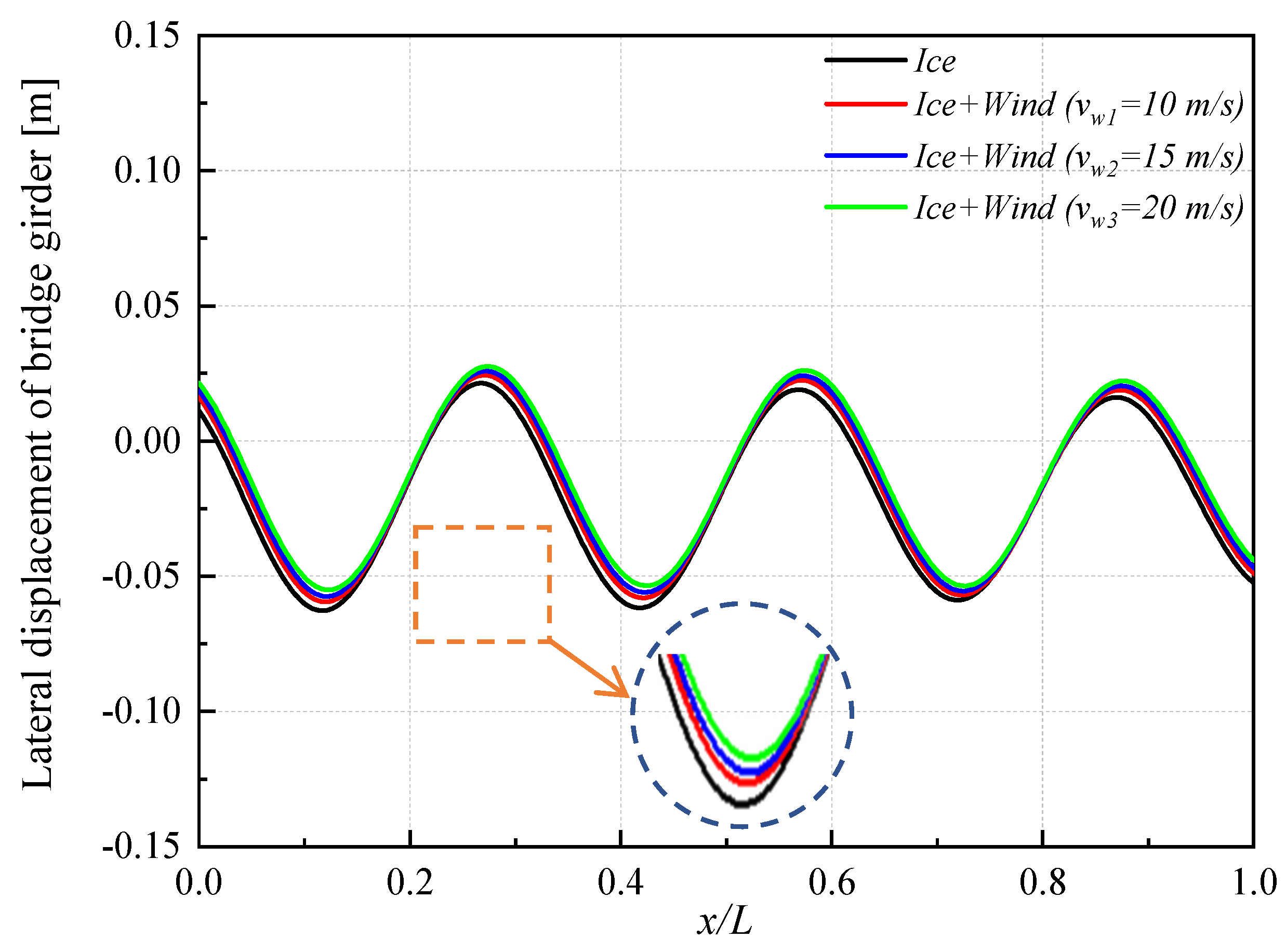
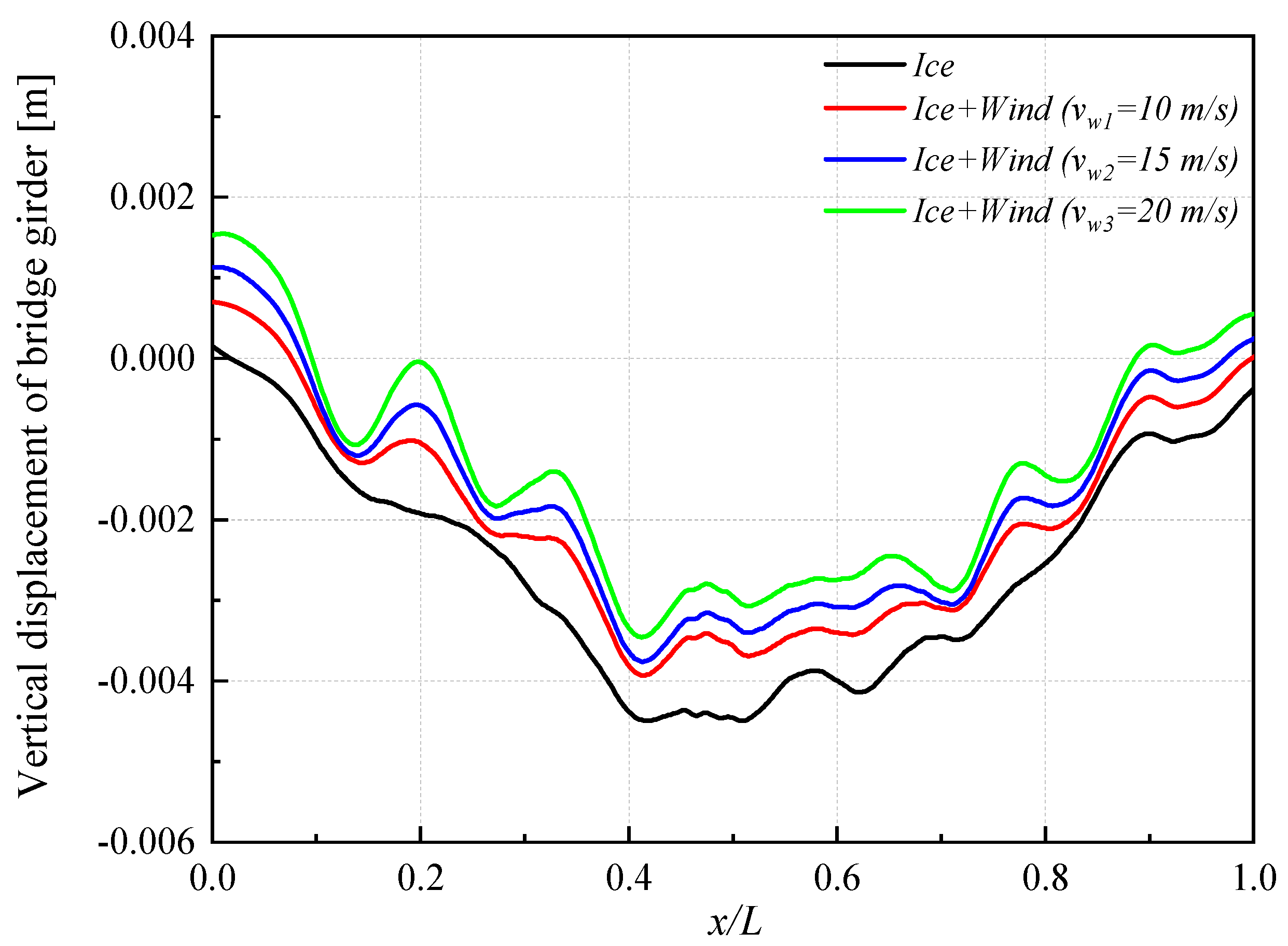
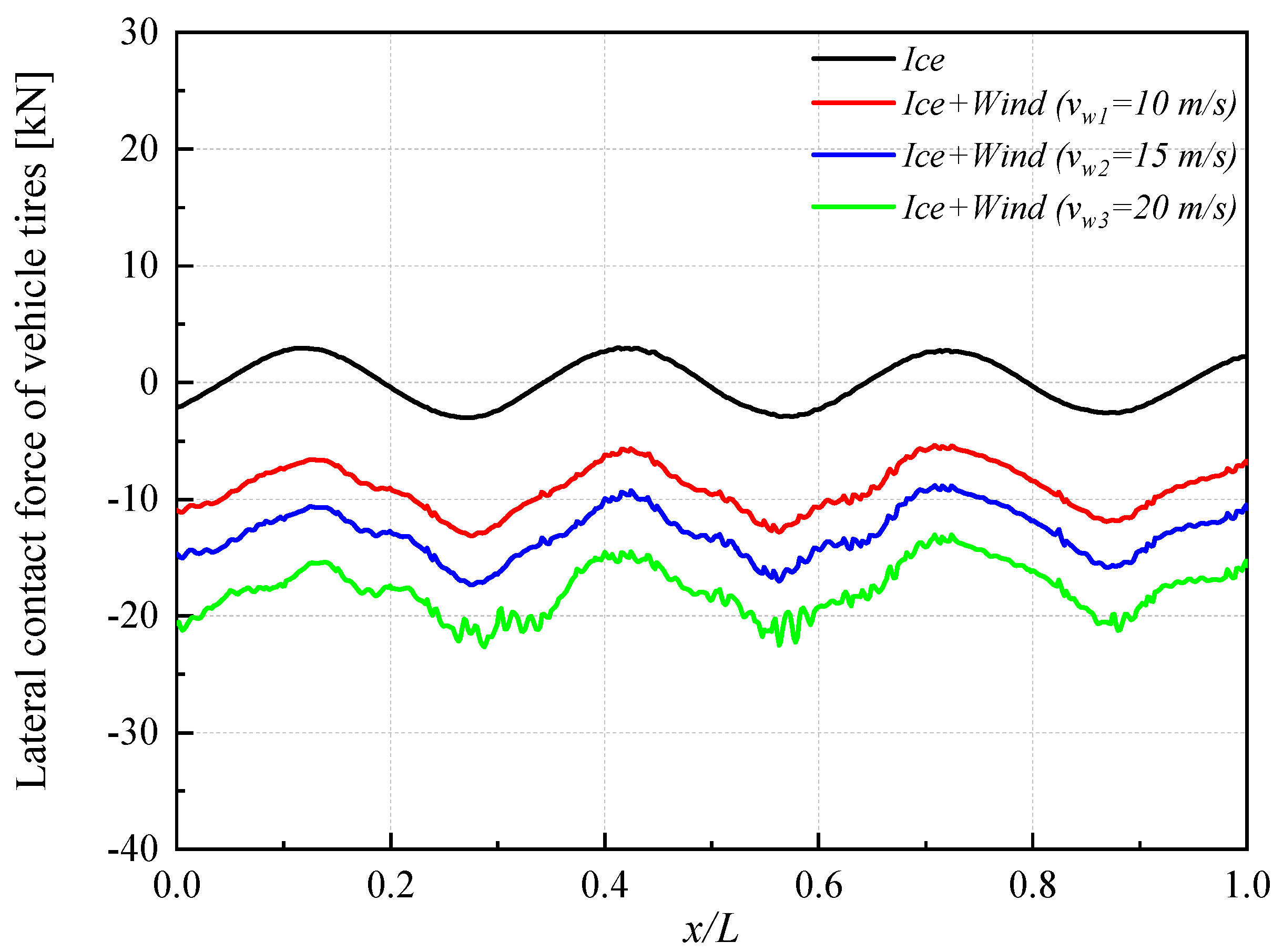
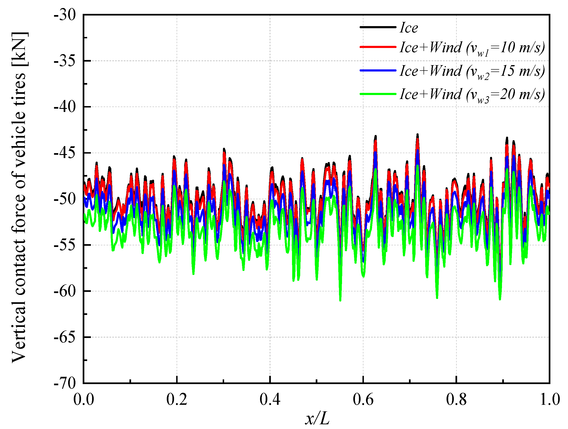
4.2. Influence of Combined Ice and Wind Loads on Dynamic Responses

In order to investigate the influence of combined ice and wind loads on the vehicle–bridge interaction system, the following analysis adopts the ice velocity of 0.6 m/s. The wind velocities are set as 10, 15, and 20 m/s to study the influence trend of wind load under the combined action of ice and wind. The lateral displacement of the bridge girder under combined ice and wind loads is shown in Figure 15. It can be seen from Figure 15 that the maximum lateral displacement of the bridge girder under ice load is greater than that under combined ice and wind loads. Although the ice and wind loads are imposed along the same direction of the transverse bridge, the lateral dynamic response of the bridge is not a simple linear superposition of the displacement caused by ice and wind loads. It can be interpreted as when the ice load is applied to the pile cap of the bridge substructure, the movement direction of the girder of the bridge superstructure is opposite to the application direction of the ice load. The wind load is directly applied to the bridge girder, and the motion direction of the bridge girder under the wind load is the same as the application direction of the wind load. Therefore, the combined action of ice and wind loads has no superposition effect on the movement of the bridge girder but has a restraining effect in the opposite direction. In addition, it can be found that the girder maximum displacement decreases with the increase in wind velocity. For example, when the wind velocities are 0, 10, 15, and 20 m/s, the maximum lateral displacements are 62.75, 59.46, 57.51, and 55.05 mm, respectively. This again shows that the wind load and ice load have opposite contributions to the motion of the bridge girder. However, from the results, ice load has a greater impact on the dynamic response of the bridge girder than wind load.

Figure 16 shows the vertical displacement of the bridge girder under combined ice and wind loads. It can be seen that the vertical displacement of the bridge girder under ice load is greater than that of under combined ice and wind loads. It can be interpreted as the ice load is only applied to the transverse bridge, which has little contribution to the vertical vibration of the bridge. However, wind load on the bridge includes the lifting force applied on the bridge girder, which can reduce the vertical displacement of the bridge girder. It can also be found that due to the increase in wind velocity, the lifting force on the bridge girder also increases, which makes the vertical displacement of the bridge girder show a decreasing trend.

Figure 17 shows the lateral contact force between vehicle tires and bridge deck under combined ice and wind loads. It can be clearly seen from Figure 17 that when only ice load acts on the bridge, the lateral contact force of the vehicle fluctuates at a lower average level. This is because when there is no transverse wind load acting on the bridge, the vehicle movement only occurs with the transverse vibration of the ice-induced bridge. However, when considering the combined effect of ice and wind loads on the bridge, it can be found that the lateral contact force of the vehicle increases significantly and fluctuates at a higher average level. For example, when the wind velocities are 0, 10, 15, and 20 m/s, the average value of lateral contact force are 1.75, 9.09, 12.91, and 17.77 kN, respectively. This also shows that with the increase in wind velocity, the lateral contact force of the vehicle will also increase, which is very unfavorable to driving safety.

The vertical contact force between vehicle tires and bridge deck under combined ice and wind loads is shown in Figure 18. It can be seen from Figure 18 that the vertical contact force of the vehicle under the combined ice and wind loads is slightly larger than that under the ice load. The vertical contact force of the vehicle is mainly affected by the pavement roughness, but the wind load also has a certain impact on the vertical contact force of the vehicle. With the increase in wind velocity, the vertical contact force of the vehicle increases slightly.

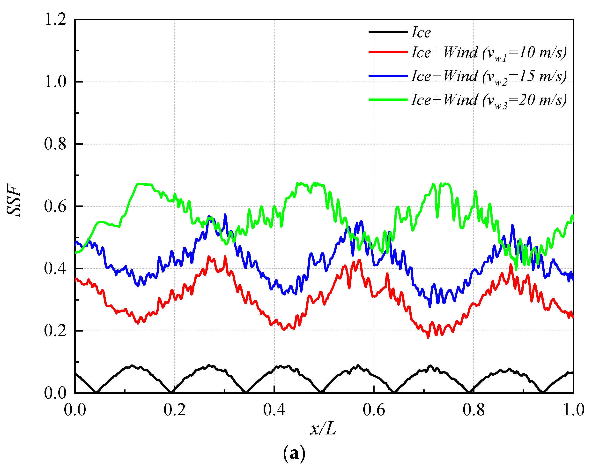
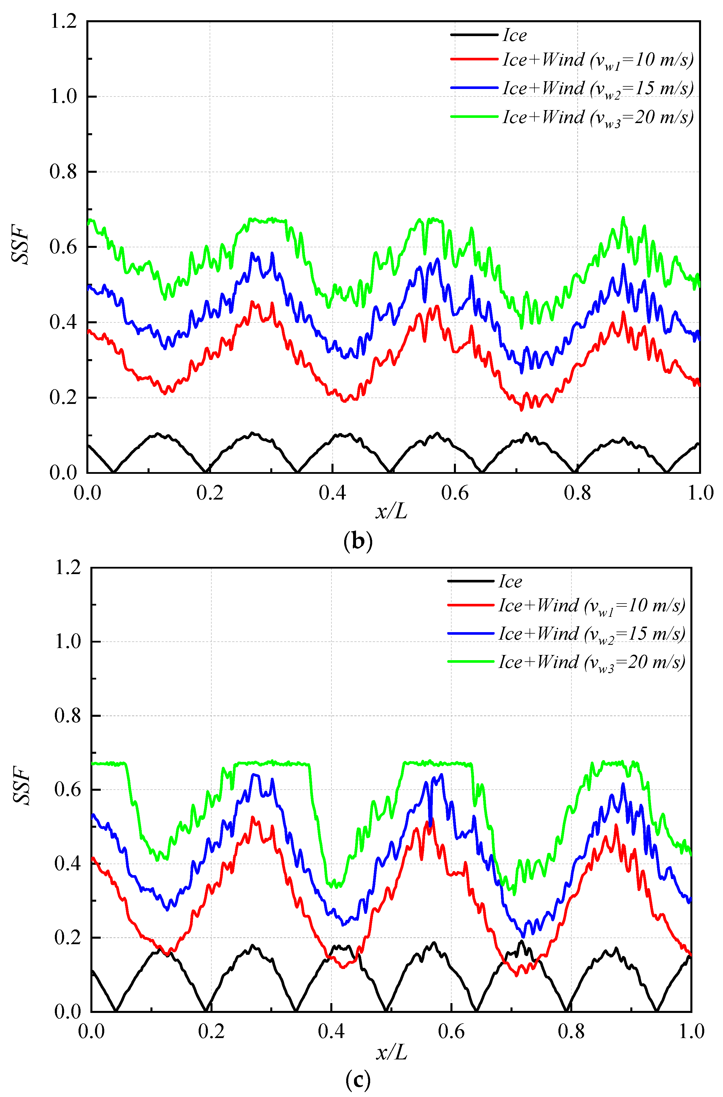
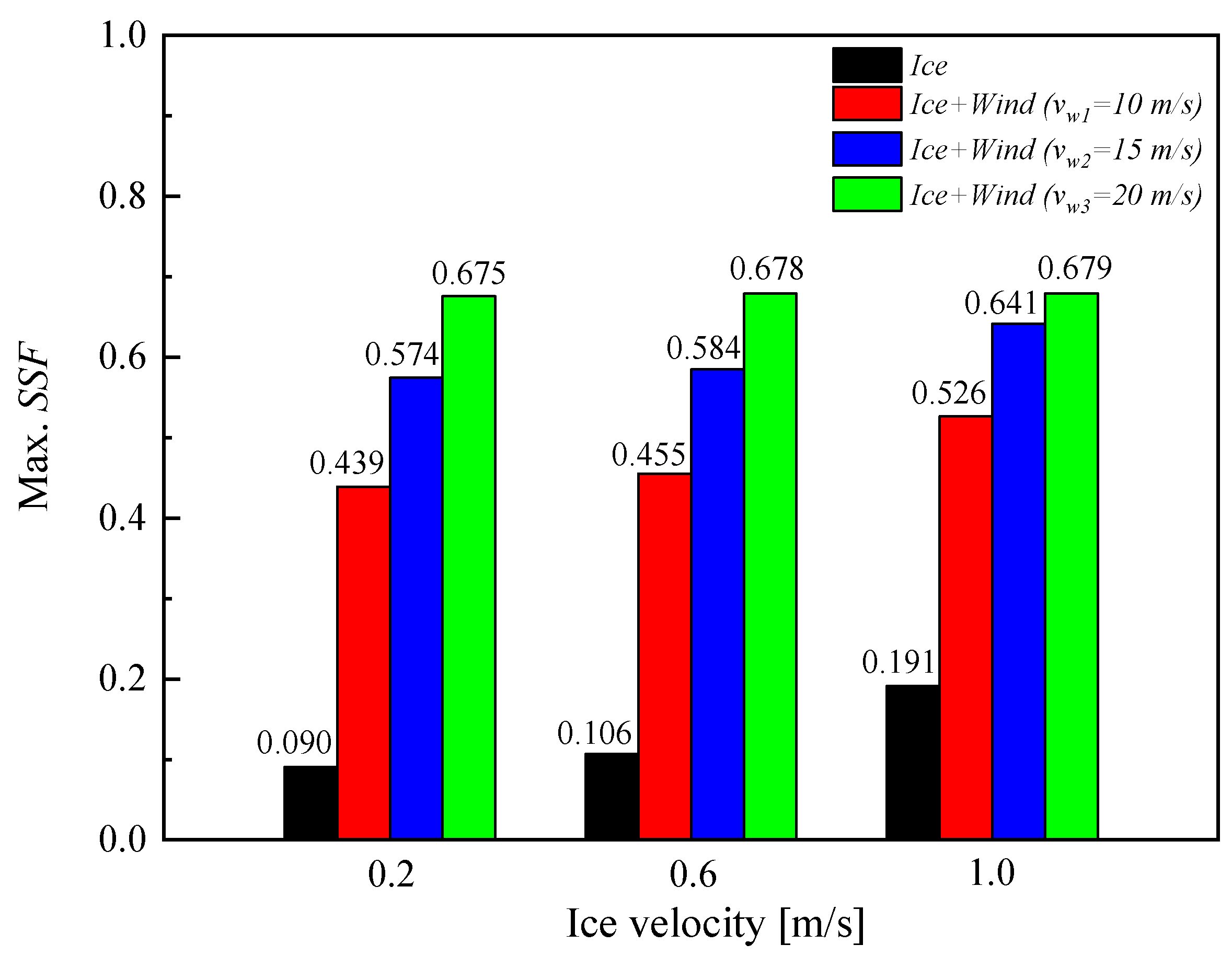
4.3. Sideslip Risk Assessment

Because ice load has little impact on vertical force of the tires on both sides of the vehicle, it has little impact on the vehicle roll problem. Therefore, this study focuses on the sideslip safety of the vehicle related to the lateral contact force of vehicles.

Road vehicles running on the bridge are prone to sideslip safety accidents under cross loads. In order to evaluate the sideslip safety more intuitively, this study uses the sideslip safety factor (SSF) to quantify the sideslip risk of the vehicle. If the value is greater than 1, the vehicle will have a sideslip accident. The SSF can be expressed as:

$$SSF=\left|\frac{F_{x,left}+F_{x,right}}{{\mu }_d\left(F_{z,left}+F_{z,right}\right)}\right|<1$$

(29)

in which F_z,left and F_z,right represent the vertical contact force of the left and right wheels at a certain axle. F_x,left and F_x,right represent the lateral contact force of the left and right wheels at a certain axle. ${\mu }_d$ denotes the friction coefficient between the tires and deck, ${\mu }_d$ = 0.6 is adopted in this study.

Figure 19a–c shows the SSF of the vehicle traveling on the bridge under combined ice and wind loads. It can be seen that the SSF of the vehicle is small, and the driving safety is good when the bridge is subjected to ice load. With the increase in ice velocity, the SSF tends to increase. This is due to the increase in ice velocity makes the bridge girder subject to greater lateral force, and the greater lateral contact force results in a greater SSF value. However, it can be seen from Figure 19 that the maximum SSF does not exceed 0.2 when the ice velocity reaches 1.0 m/s, which proves that the SSF of the vehicle still has at least an 80% margin even under the condition of fast ice velocity. In addition, it can be found that the SSF under combined ice and wind loads is much higher than that under ice load. With the increase in wind velocity, the SSF of the vehicle shows a significant increase trend. It can also be found that with the increase in ice velocity, the fluctuation range of SSF at the same wind velocity also expands. This also proves that the coupling effect of ice load and wind load will affect the SSF of the vehicle. It can be seen from Figure 19 that the maximum SSF reaches 0.679 when the ice velocity reaches 1.0 m/s and the SSF of the vehicle is only about 30% margin.

Figure 20 shows the maximum SSF of the vehicle traveling on the bridge under various conditions.

Table 1. The maximum SSF of the vehicle and difference under various conditions.

Wind Velocity [m/s]	Ice Velocity [m/s]
	vi1 = 0.2	vi2 = 0.6		vi3 = 1.0
	Max. SSF	Max. SSF	Difference [%]	Max. SSF	Difference [%]
vw0 = 0	0.09	0.106	17.77	0.191	112.22
vw1 = 10	0.439	0.455	3.64	0.526	19.81
vw2 = 15	0.574	0.584	1.74	0.641	11.67
vw3 = 20	0.675	0.678	0.44	0.679	0.59

lists the maximum SSF of the vehicle and difference under various conditions. It can be clearly seen that the maximum SSF of the vehicle is under different conditions when ice and wind loads are combined. The maximum SSF of the vehicle increases with the increase in ice velocity when the ice load acts on the bridge. When the ice velocity is 0.6 and 1.0 m/s, the maximum SSF of the vehicle is 0.106 and 0.191, respectively, which is 17.77% and 112.22% higher than 0.090 when the ice velocity is 0.2 m/s. It can be seen that the higher the ice velocity is, the worse the driving safety will be. The maximum SSF of the vehicle increases with the increase in wind velocity under combined ice and wind loads and is significantly larger than the maximum SSF under ice load. In addition, it can be found that with the increase in ice velocity, the maximum SSF at the same wind velocity also shows an increasing trend. For example, when the ice velocity is 0.6 and 1.0 m/s, the maximum SSF of the vehicle at 15 m/s wind velocity is 0.584 and 0.641, respectively, which is 1.74% and 11.67% higher than 0.574 when the ice velocity is 0.2 m/s. However, the impact of ice velocity on the maximum SSF of the vehicle decreases gradually with the increase in wind velocity. It can be found that the maximum SSF difference under various ice velocities is very small when wind velocity rises to 20 m/s. This also shows that the driving safety of the ice–wind–vehicle–bridge interaction system is mainly controlled by wind load, but the combined impact of ice and wind loads on driving safety cannot be ignored.

5. Conclusions

There is a harsh working environment for sea-crossing bridges in cold sea regions. As well as being able to withstand the impact of ice load, it must also take into account the combined effect of strong wind. This poses a great threat to the safe driving operation of vehicles. This study constructs a complete framework of ice–wind–vehicle–bridge interaction to investigate vibration under combined ice and wind loads. Ice load is simulated by a linearized ice–structure interaction model, which is based on the self-excited vibration theory. The wind load on the vehicle is calculated based on the quasi-steady model. The static aerodynamic coefficient of girder is obtained through the wind tunnel test and wind loads, including steady-state force and buffering force, are further obtained. The proposed analysis framework is then applied to an offshore bridge with running road vehicles in the Bohai Sea. The conclusions are as follows:

The ice load has a greater influence on the lateral dynamic response of the bridge, while the wind load has a more significant influence on the lateral dynamic response of the vehicle. Due to the different action characteristics of ice load and wind load on the vehicle–bridge interaction system, the lateral dynamic responses of the bridge and vehicle under separate ice and wind loads cannot be combined by superposition. In short, ice and wind loads affect the vehicle–bridge interaction system in different ways, so it is very meaningful to consider the dynamic coupling effect of ice and wind on the vehicle–bridge interaction system.

The combined action of ice and wind has a great influence on the sideslip safety factor (SSF) of a vehicle. Compared with ice load, wind load has a greater impact on the sideslip safety, but the combined impact of ice load and wind load on driving safety cannot be ignored. The combined action of ice and wind should be reasonably considered in the driving safety analysis of sea-crossing bridges in ice-covered waters.

It should be noted that the concluding remarks presented above were based on specific self-induced ice loads and the bridge type considered in this study. The wind load on the bridge is also generated based on the main beam section of the case bridge in this study. Additional investigations of different bridges and vehicles should be carried out before common concluding remarks can be drawn. The results of coupled vibration response of the ice–wind–vehicle–bridge interaction system should be further verified by experiments or more refined numerical methods.

References

1. Yang, Y.B.; Lin, B.H. Vehicle-bridge interaction analysis by dynamic condensation method. J. Struct. Eng. 1995, 121, 1636–1643. [Google Scholar] [CrossRef]
2. Neves, S.G.M.; Azevedo, A.F.M.; Canada, R. A direct method for analyzing the vertical vehicle-structure interaction. Eng. Struct. 2012, 34, 414–420. [Google Scholar] [CrossRef] [Green Version]
3. Lu, X.Z.; Kim, C.W.; Chang, K.C. Finite element analysis framework for dynamic vehicle-bridge interaction system based on ABAQUS. Int. J. Struct. Stab. Dyn. 2020, 4, 2050034. [Google Scholar] [CrossRef]
4. Yang, Y.B.; Yau, J.D. Vehicle-bridge interaction element for dynamic analysis. J. Struct. Eng. 1997, 11, 1512–1518. [Google Scholar] [CrossRef]
5. Camara, A.; Kavrakov, I.; Nguyen, K.; Morgenthal, G. Complete framework of wind-vehicle-bridge interaction with random road surfaces. J. Sound Vib. 2019, 458, 197–217. [Google Scholar] [CrossRef]
6. Xie, J.J.; Li, J.; Tian, Z.; Zhen, L.X.; Gu, Y.; Lao, X.D.; Zhang, C.G. Dynamic response analysis of vehicles crossing a bridge considering the randomness of road surface roughness. J. Vib. Shock 2021, 40, 299–306. [Google Scholar]
7. Li, Y.L.; Chen, N.; Zhao, K. Seismic response analysis of road vehicle–bridge system for continuous rigid frame bridges with high piers. Earthq. Eng. Eng. Vib. 2012, 11, 593–602. [Google Scholar] [CrossRef]
8. Wang, Y.W.; Zheng, K.F.; Xiong, Z.L.; Zhu, J.; Feng, X.-Y.; Lei, M. Coupled vibration analysis of vehicle-bridge foe long-span bridge under wind and earthquake action. China J. Highw. Transp. 2021, 34, 298–308. [Google Scholar]
9. Paraskeva, T.S.; Dimitrakopoulos, E.G.; Zeng, Q. Dynamic vehicle-bridge interaction under simultaneous vertical earthquake excitation. Bull. Earthq. Eng. 2016, 15, 71–95. [Google Scholar] [CrossRef]
10. Zhou, Y.; Chen, S. Fully coupled driving safety analysis of moving traffic on long-span bridges subjected to crosswind. J. Wind Eng. Ind. Aerodyn. 2015, 143, 1–18. [Google Scholar] [CrossRef] [Green Version]
11. Xu, Y.L.; Guo, W.H. Dynamic analysis of coupled road vehicle and cable-stayed bridge systems under turbulent wind. Eng. Struct. 2003, 25, 473–486. [Google Scholar] [CrossRef]
12. Han, Y.; Cai, C.S.; Zhang, J.; Chen, S.; He, X. Effects of aerodynamic parameters on the dynamic responses of road vehicles and bridges under cross winds. J. Wind Eng. Ind. Aerodyn. 2014, 134, 78–95. [Google Scholar] [CrossRef]
13. Guo, W.H.; Xu, Y.L. Safety analysis of moving road vehicles on a long bridge under crosswind. J. Eng. Mech. 2006, 132, 438–446. [Google Scholar] [CrossRef]
14. Xia, C.Y. Dynamic Responses of Train-Bridge System Subjected to Collision Loads and Running Safety Evaluation of High-Velocity Trains. Ph.D. Thesis, Beijing Jiaotong University, Beijing, China, 2012. [Google Scholar]
15. Xia, C.Y.; Lei, J.Q.; Zhang, N.; Xia, H.; De Roeck, G. Dynamic analysis of a coupled high-velocity train and bridge system subjected to collision load. J. Sound Vib. 2011, 331, 2334–2347. [Google Scholar] [CrossRef]
16. Wu, T.Y.; Qiu, W.L.; Kim, C.W.; Chang, K.C.; Lu, X.Z. Dynamic responses of a vehicle-bridge-soil interaction system subjected to stochastic-type ice loads. Struct. Infrastruct. Eng. 2021, 2023586, 1–20. [Google Scholar] [CrossRef]
17. Zhou, Y.F.; Chen, S.R. Vehicle ride comfort analysis with whole-body vibration on longspan bridges subjected to crosswind. J. Wind Eng. Ind. Aerodyn. 2016, 155, 126–140. [Google Scholar] [CrossRef] [Green Version]
18. Goyal, A.; Chopra, A.K. Simplified evaluation of added hydrodynamic mass for intake towers. J. Eng. Mech. 1989, 11, 1393–1412. [Google Scholar] [CrossRef]
19. Zuo, H.; Bi, K.; Hao, H. Dynamic analyses of operating offshore wind turbines including soil-structure interaction. Eng. Struct. 2018, 157, 42–62. [Google Scholar] [CrossRef]
20. DNV-OS-J101; Design of Offshore Wind Turbine Structures. Det Norske Veritas: Oslo, Norway, 2010.
21. Wu, T.Y.; Qiu, W.L. Dynamic analyses of pile-supported bridges including soil-structure interaction under stochastic ice loads. Soil Dyn. Earthq. Eng. 2020, 128, 105879. [Google Scholar] [CrossRef]
22. ISO-8608; Mechanical Vibration-Road Surface Profiles-Reporting of Measured Data. International Organization for Standardization-8608: Geneva, Switzerland, 1995.
23. Dodds, C.J.; Robson, J.D. The description of road surface roughness. J. Sound Vib. 1973, 31, 175–183. [Google Scholar] [CrossRef]
24. Wang, H.; Mao, J.X.; Spencer, B.F. A monitoring-based approach for evaluating dynamic responses of riding vehicle on long-span bridge under strong winds. Eng. Struct. 2019, 189, 35–47. [Google Scholar] [CrossRef]
25. Peri, D.; Owen, D.R.J. Computational model for 3-D contact problems with friction based on the penalty method. Int. J. Numer. Methods Eng. 1992, 35, 1289–1309. [Google Scholar] [CrossRef]
26. Hunˇek, I. On a penalty formulation for contact-impact problems. Comput. Struct. 1993, 48, 193–203. [Google Scholar] [CrossRef]
27. Määttänen, M. On Conditions for the Rise of Self-Excited Ice-Induced Autonomous Oscillations in Slender Marine Pile Structures. Winter Navigation Research Board: Helsinki, Finland, 1978. [Google Scholar]
28. Wang, L.Y.; Xu, J.Z. Theoretical analysis model of dynamic interaction between ice and structure. Haiyang Xuebao 1993, 3, 140–146. [Google Scholar]
29. Wright, B. Insights from Molikpaq Ice Loading Data. In Validation of Low Level Ice Forces on Coastal Structures; Report LOLEIF Report No. 1, EU Project, Contract MAS3-CT 97-0098; HSVA: Hamburg, Germany.
30. Palmer, A.C.; Goodman, D.J.; Ashby, M.F.; Evans, A.G.; Hutchinson, J.W.; Ponter, A.R.S. Fracture and its role in determining ice forces on offshore structures. Ann. Glaciol. 1983, 4, 216–221. [Google Scholar] [CrossRef] [Green Version]
31. Eivind, S.L. Numerical Modelling of Ice Induced Vibrations of Lock-In Type; Norwegian University of Science and Technology: Trondheim, Norway, 2014. [Google Scholar]
32. Chen, N.; Li, Y.; Wang, B.; Su, Y.; Xiang, H. Effects of wind barrier on the safety of vehicles driven on bridges. J. Wind Eng. Ind. Aerodyn. 2015, 143, 113–127. [Google Scholar] [CrossRef]
33. Scanlan, R.H.; Jones, N.P. Aeroelastic analysis of cable-stayed bridges. J. Struct. Eng. 1990, 116, 279–297. [Google Scholar] [CrossRef]
34. Ji, S.Y.; Yue, Q.J.; Bi, X.J. Probability distribution of sea ice fatigue parameters in JZ20-2 sea area of the Liaodong Bay. Ocean Eng. 2002, 20, 39–43. [Google Scholar]
35. Ji, S.Y.; Yue, Q.J. Monte-Carlo simulation of fatigue ice load for offshore platform with ice-broken gone in the Liaodong gulf. Haiyang Xuebao 2003, 25, 114–119. [Google Scholar]
Figure 1. Schematic of simulation process for ice–wind–vehicle–bridge interaction.
Jmse 11 00535 g001
Figure 2. The high-sided road truck, (a) elevation view, (b) side view, (c) plan view.
Jmse 11 00535 g002aJmse 11 00535 g002b
Figure 3. Overall layout diagram of the bridge in this study (unit: m).
Jmse 11 00535 g003
Figure 4. Layout diagram of cross-section of the girder in this study (unit: m).
Jmse 11 00535 g004
Figure 5. Layout diagram of pier and foundation of the bridge in this study (unit: cm).
Jmse 11 00535 g005
Figure 6. Nonlinear soil springs in this study, (a) p-y curve, (b) t-z curve, (c) Q-z curve.
Jmse 11 00535 g006aJmse 11 00535 g006b
Figure 7. Simulated road irregularities in this study.
Jmse 11 00535 g007
Figure 8. Finite element model of vehicle–bridge coupling system in ABAQUS. (a) Truck model, (b) vehicle–bridge interaction model.
Jmse 11 00535 g008
Figure 9. Flow chart of time integration for ice–wind–vehicle–bridge interaction system.
Jmse 11 00535 g009
Figure 10. Linearized ice-crushing strength versus stress rate.
Jmse 11 00535 g010
Figure 11. Segment model of the girder of the sea-crossing bridge in wind tunnel laboratory.
Jmse 11 00535 g011
Figure 12. The measured aerodynamic force coefficients of the bridge with different attack angles, (a) drag coefficient, (b) lift coefficient, (c) moment coefficient.
Jmse 11 00535 g012
Figure 13. Lateral displacement of bridge girder under various ice velocities.
Jmse 11 00535 g013
Figure 14. Lateral contact force between vehicle tires and bridge deck under various ice velocities.
Jmse 11 00535 g014
Figure 15. Lateral displacement of bridge girder under combined ice and wind loads.
Jmse 11 00535 g015
Figure 16. Vertical displacement of bridge girder under combined ice and wind loads.
Jmse 11 00535 g016
Figure 17. Lateral contact force between tires and bridge deck under combined ice and wind loads.
Jmse 11 00535 g017
Figure 18. Vertical contact force between tires and bridge deck under combined ice and wind loads.
Jmse 11 00535 g018
Figure 19. The SSF of the vehicle under combined ice and wind loads, (a) ice velocity vi = 0.2 m/s, (b) ice velocity vi = 0.6 m/s, (c) ice velocity vi = 1.0 m/s.
Jmse 11 00535 g019aJmse 11 00535 g019b
Figure 20. The maximum SSF of the vehicle under combined ice and wind loads.
Jmse 11 00535 g020