
Sparsity Regularization-Based Real-Time Target Recognition for Side Scan Sonar with Embedded GPU

Abstract
:1. Introduction
2. Relate Work
2.1. SSS Object Detection Based on Deep Learning
2.2. Computation Reduction
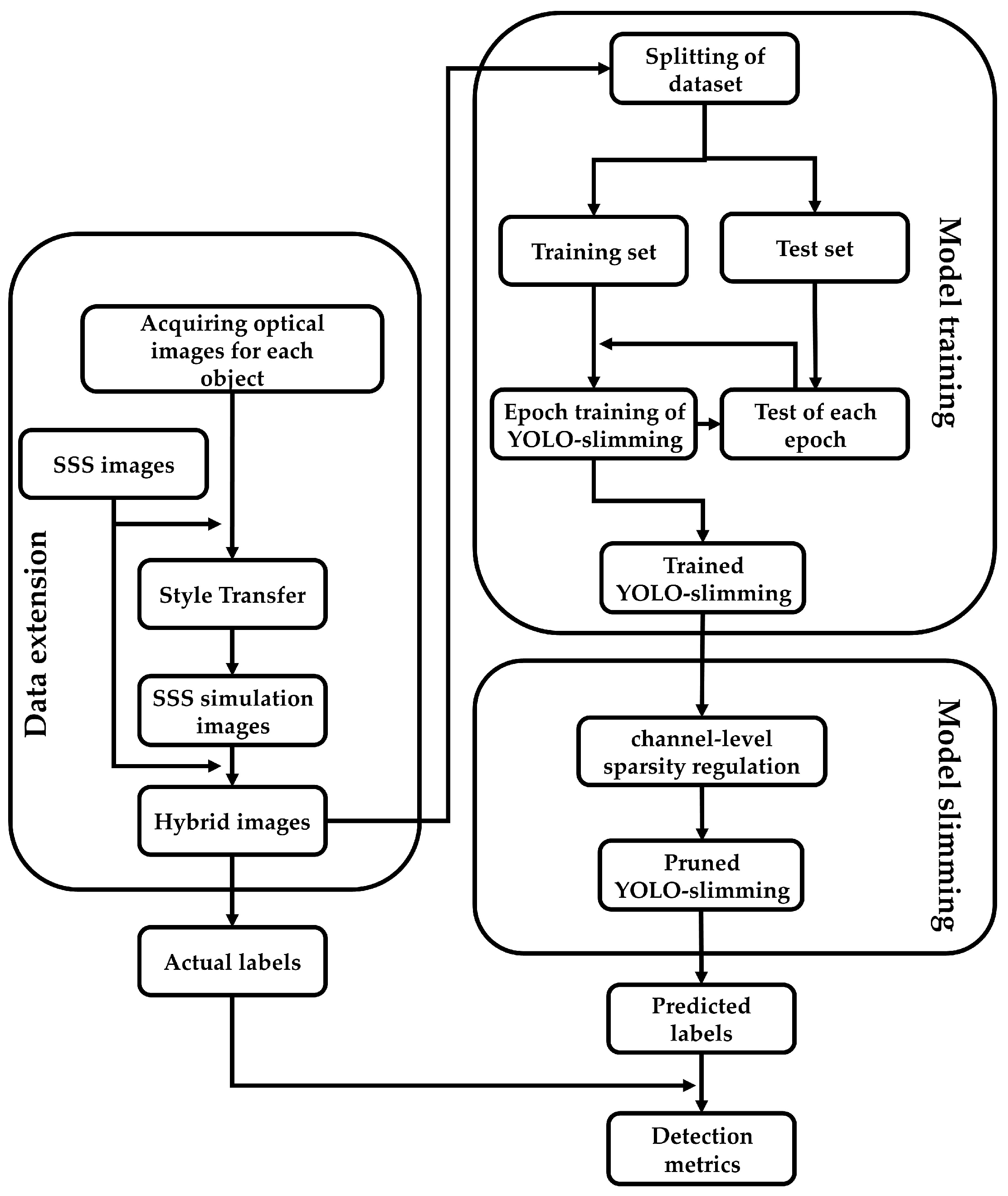
3. Methods
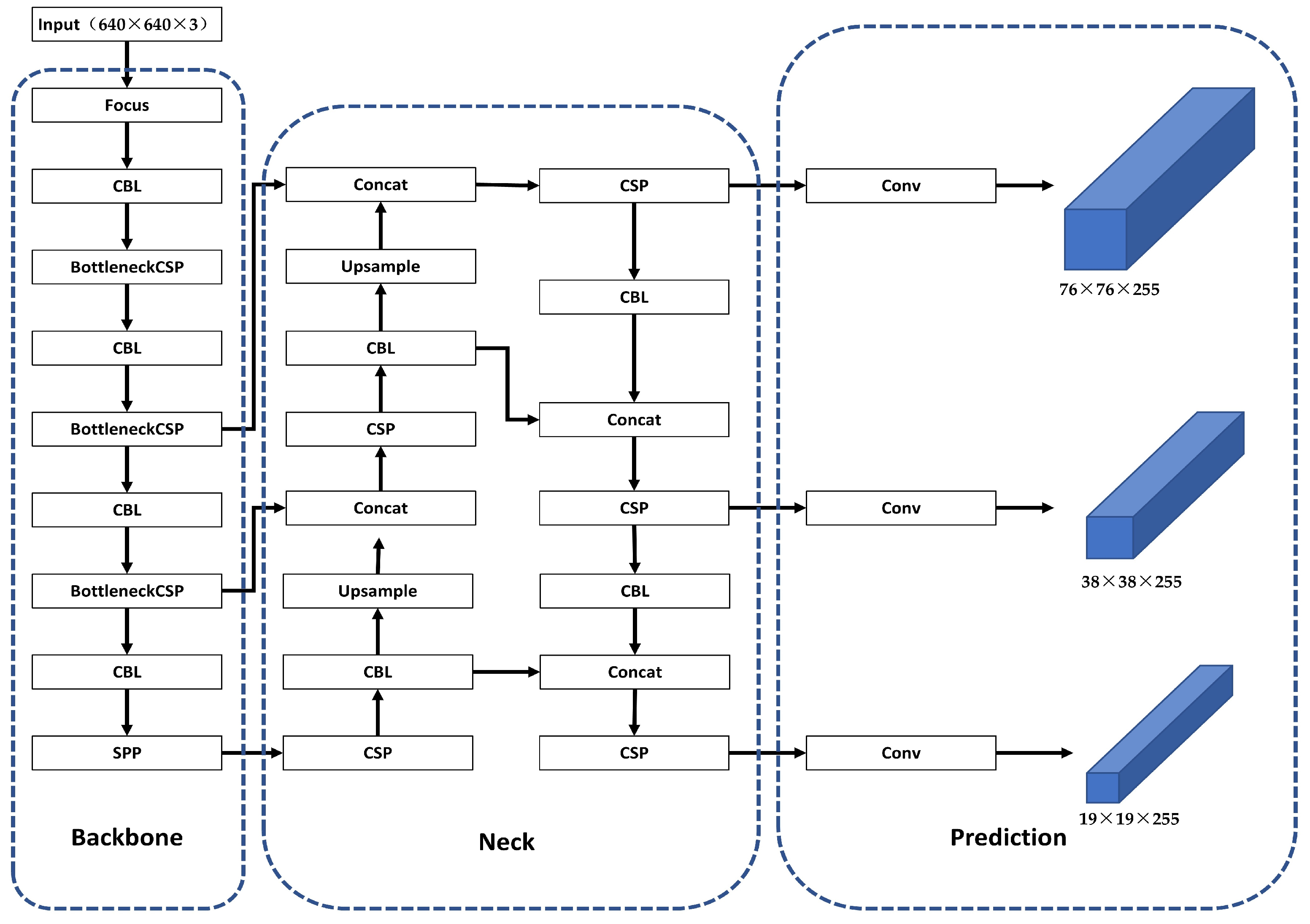
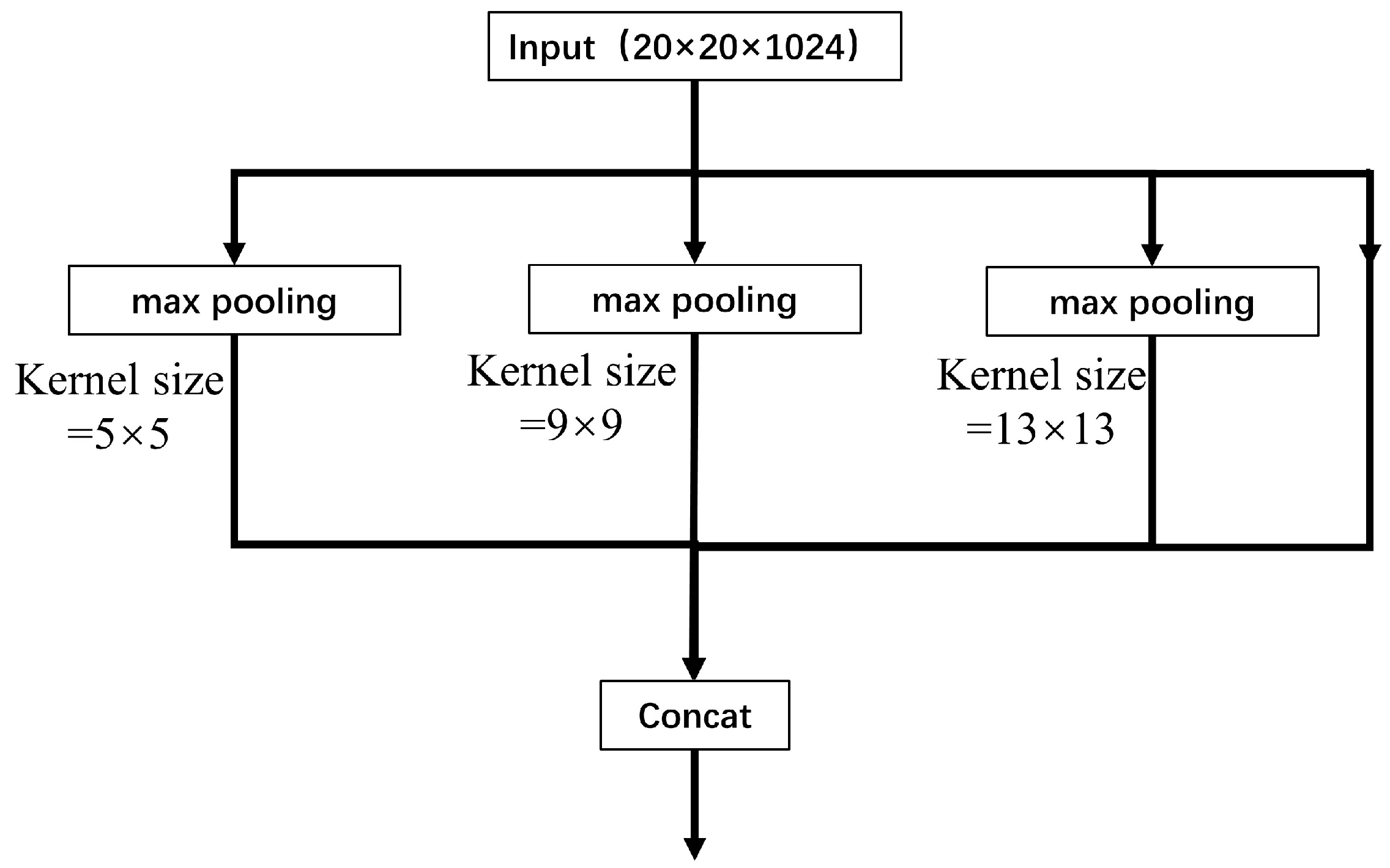
3.1. YOLOv5
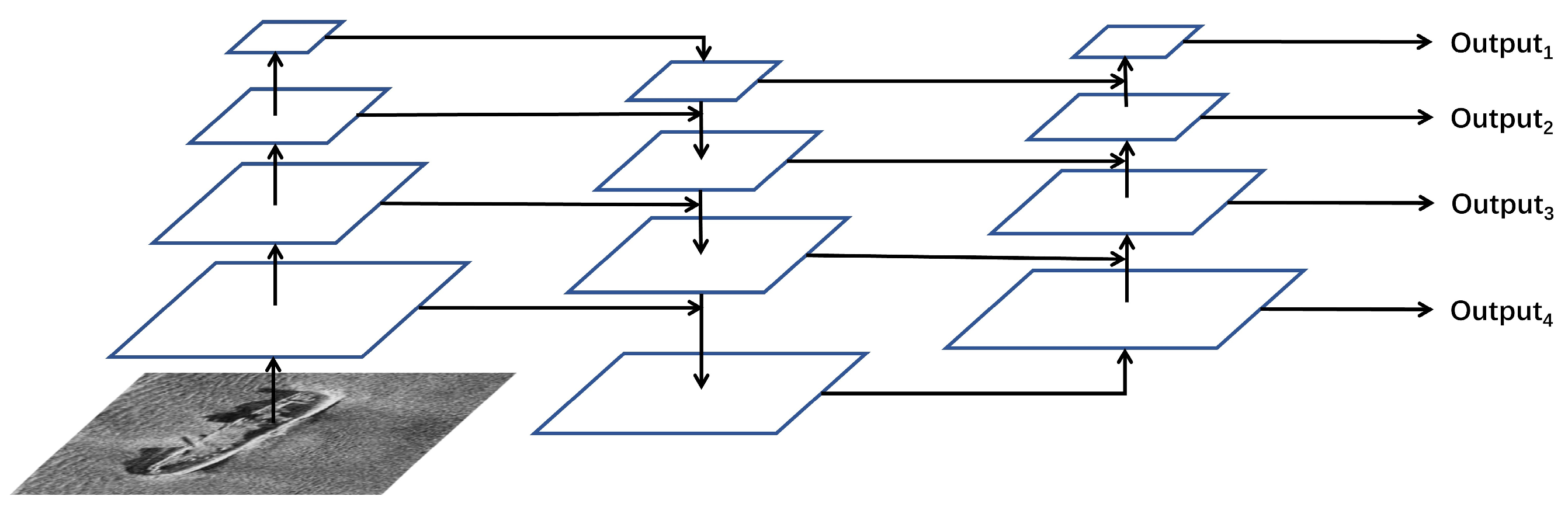
3.2. The CE Feature Encoder
3.3. Channel-Level Sparsity Regularization
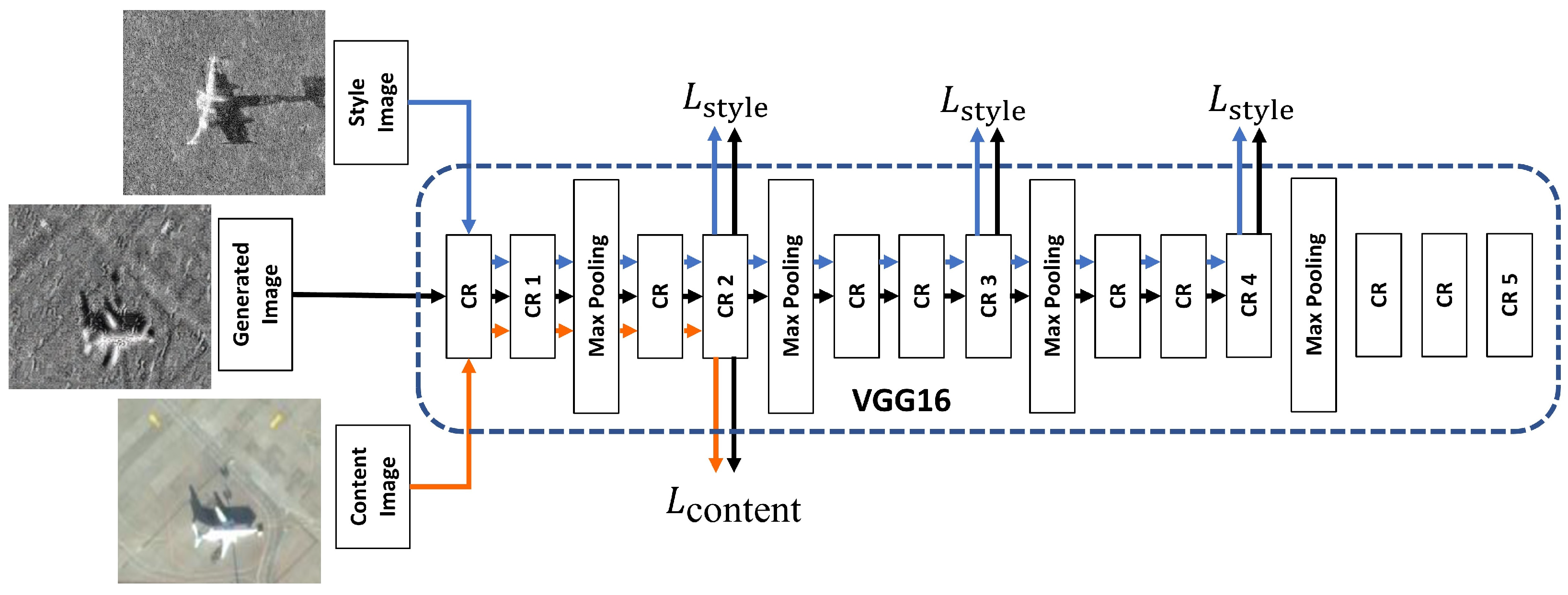
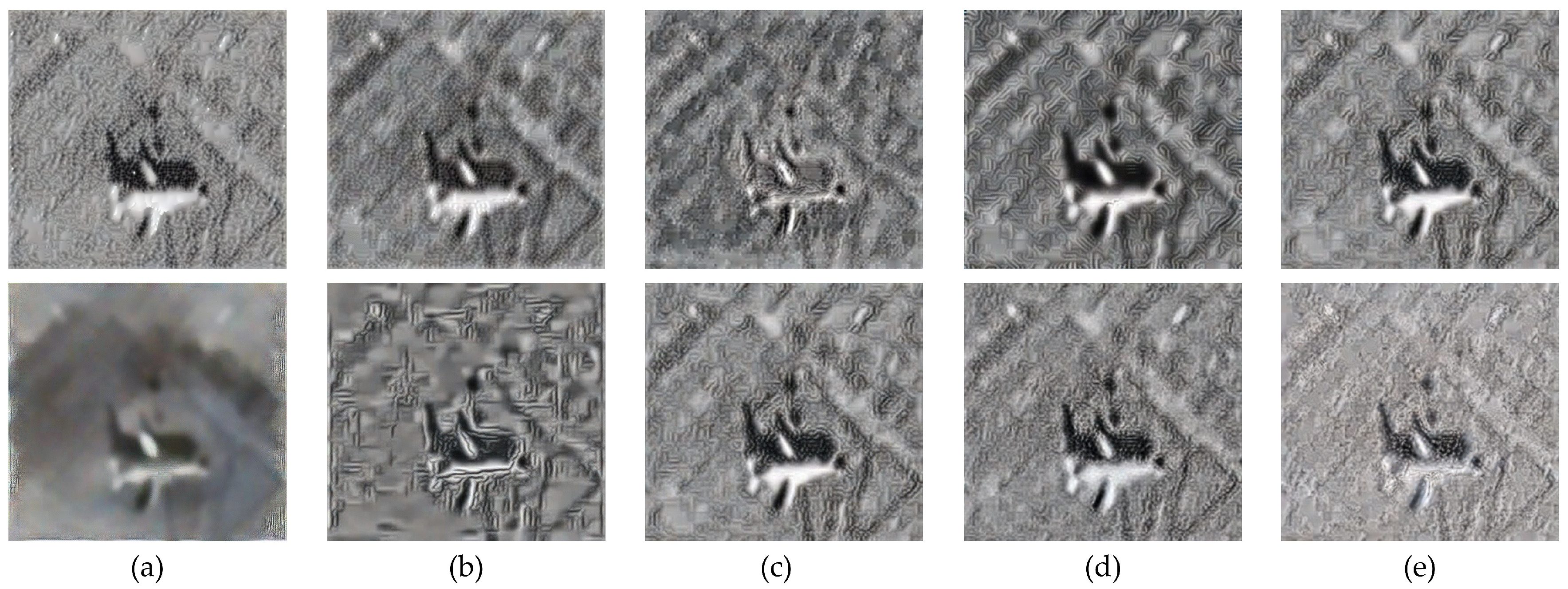
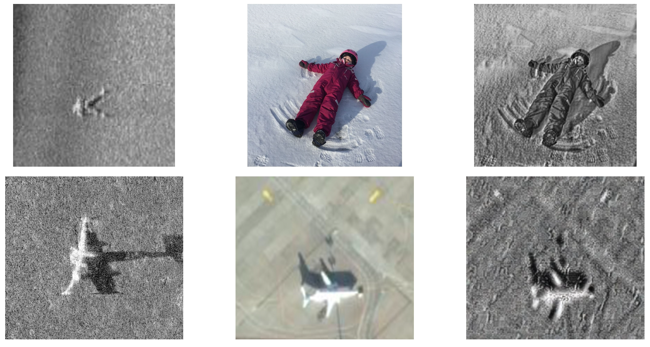
3.4. SSS Image Simulation Based on Deep Style Transfer
4. The Dataset and Training Strategy
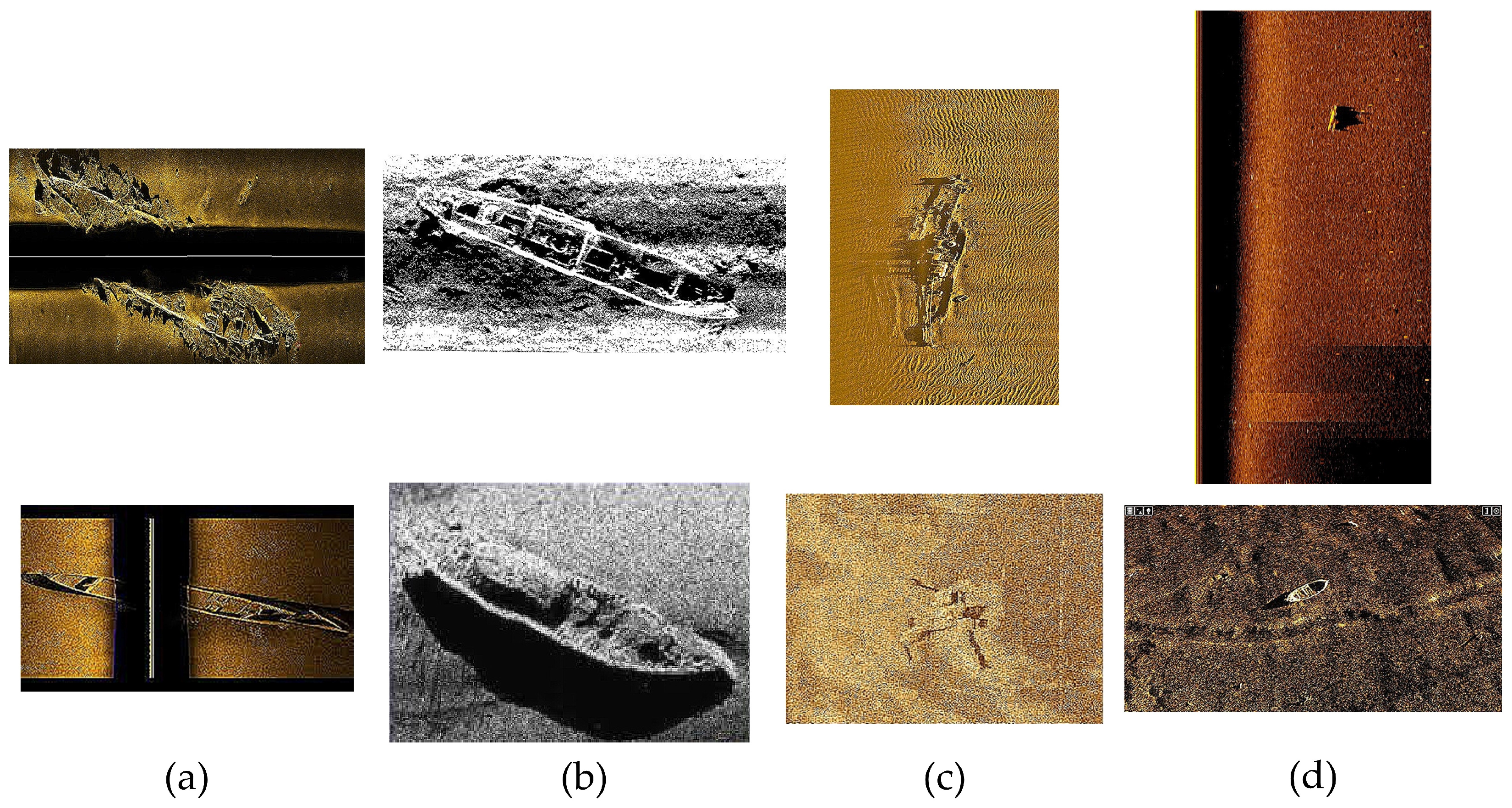
4.1. The Dataset
- SCTD has collected three types of target images, but the number of samples is unbalanced, especially since the number of images of the drowning victims is only 45.
- The detection range and imaging method of SSS are different, and interference detection such as crushing, fracture and deformation is not satisfactory.
- SCTD is collected from a variety of sources, and image size, resolution, and aspect ratio vary greatly.
4.2. Multi-Scale Images
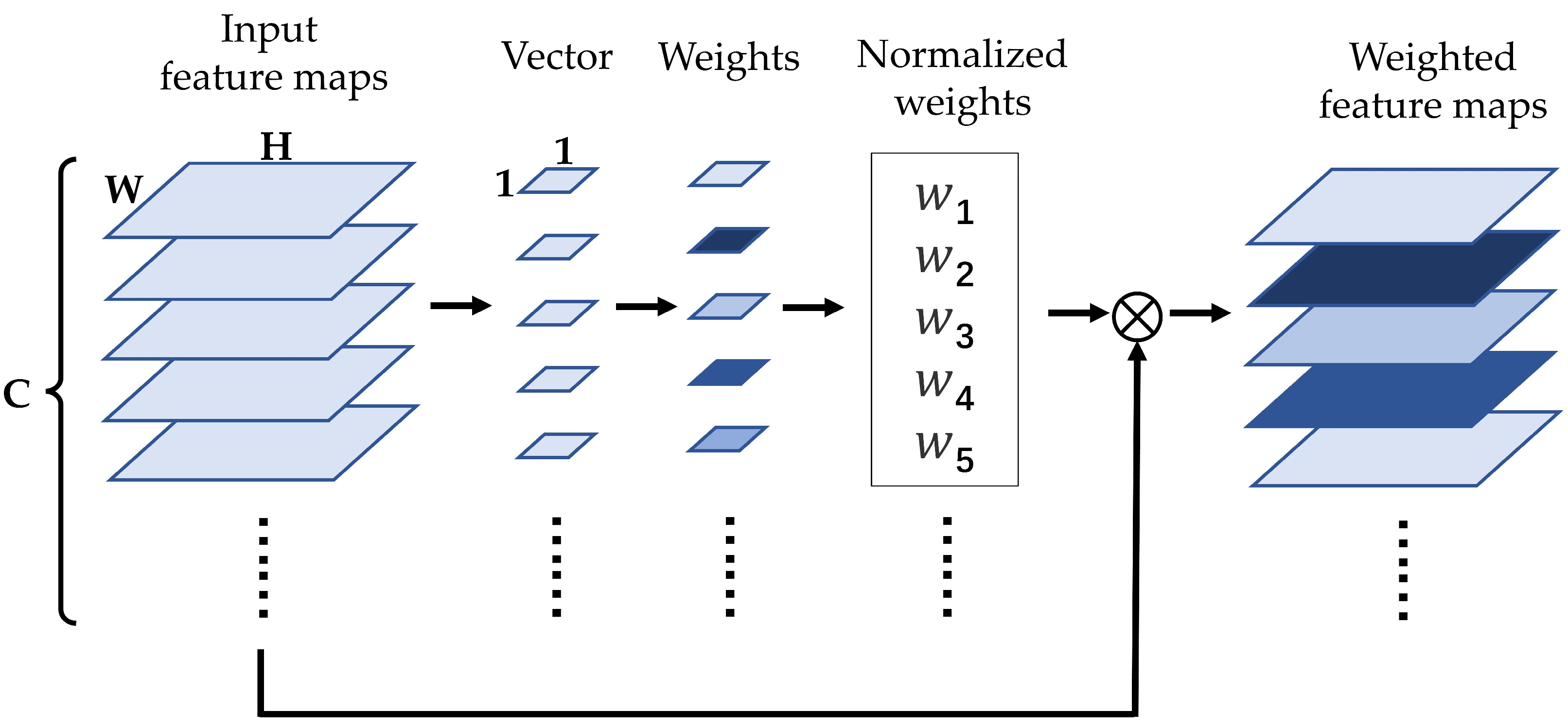
4.3. Weighted Image Selection
4.4. Mosaic Image Enhancement
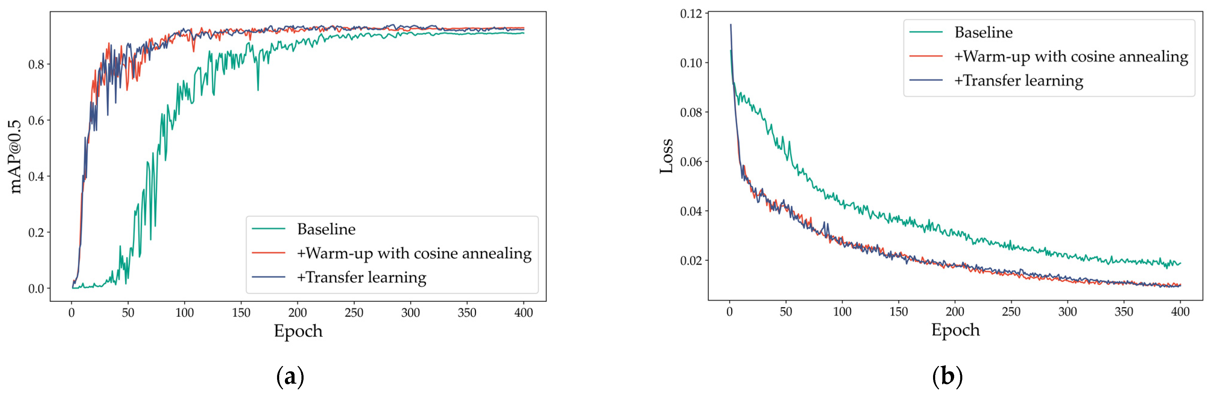
4.5. Warm-Up with Cosine Annealing
4.6. Transfer Learning
4.7. Other Training Details
5. Experiments and Analysis
5.1. Experimental Conditions
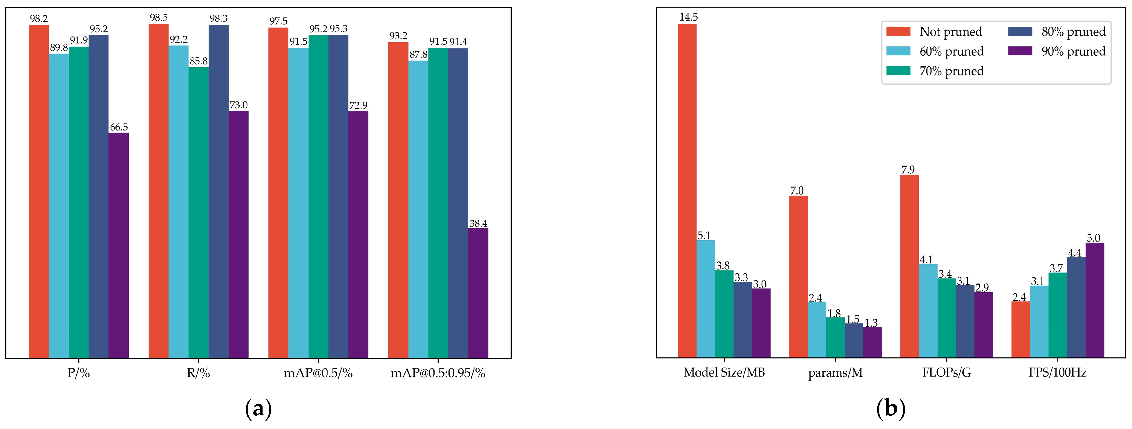
5.2. Network Accuracy Analysis
5.3. Network Complexity Analysis
5.4. Real-Time Inception
6. Conclusions
Author Contributions
Funding
Institutional Review Board Statement
Informed Consent Statement
Data Availability Statement
Acknowledgments
Conflicts of Interest
References
- Kaeser, A.J.; Litts, T.L.; Tracy, T.W. Using Low-cost Side-scan Sonar for Benthic Mapping throughout the Lower Flint River, Georgia, USA. River Res. Appl. 2013, 29, 634–644. [Google Scholar] [CrossRef]
- Kennish, M.J.; Haag, S.M.; Sakowicz, G.P.; Tidd, R.A. Side-scan sonar imaging of subtidal benthic habitats in the Mullica River Great Bay estuarine system. J. Coast. Res. 2004, 227–240. [Google Scholar] [CrossRef]
- Llorens-Escrich, S.; Tamarit, E.; Hernandis, S.; Sanchez-Carnero, N.; Rodilla, M.; Perez-Arjona, I.; Moszynski, M.; Puig-Pons, V.; Tena-Medialdea, J.; Espinosa, V. Vertical Configuration of a Side Scan Sonar for the Monitoring of Posidonia oceanica Meadows. J. Mar. Sci. Eng. 2021, 9, 1332. [Google Scholar] [CrossRef]
- Wright, R.G.; Baldauf, M. Hydrographic Survey in Remote Regions: Using Vessels of Opportunity Equipped with 3-Dimensional Forward-Looking Sonar. Mar. Geod. 2016, 39, 439–457. [Google Scholar] [CrossRef]
- LeHardy, P.K.; Moore, C. Deep Ocean Search for Malaysia Airlines Flight 370. In Proceedings of the Oceans Conference, St. John’s, NB, Canada, 14–19 September 2014. [Google Scholar]
- LeHardy, P.K.; Larsen, J. Deepwater Synthetic Aperture Sonar and the Search for MH370. In Proceedings of the OCEANS MTS/IEEE Conference, Washington, DC, USA, 19–22 October 2015. [Google Scholar]
- Pailhas, Y.; Petillot, Y.; Brown, K.; Mulgrew, B. Spatially Distributed MIMO Sonar Systems: Principles and Capabilities. IEEE J. Ocean. Eng. 2017, 42, 738–751. [Google Scholar] [CrossRef] [Green Version]
- Yu, H.P.; Li, Z.Y.; Li, D.L.; Shen, T.S. Bottom Detection Method of Side-Scan Sonar Image for AUV Missions. Complexity 2020, 2020, 9. [Google Scholar] [CrossRef]
- Grothues, T.M.; Newhall, A.E.; Lynch, J.F.; Vogel, K.S.; Gawarkiewicz, G.G. High-frequency side-scan sonar fish reconnaissance by autonomous underwater vehicles. Can. J. Fish. Aquat. Sci. 2017, 74, 240–255. [Google Scholar] [CrossRef] [Green Version]
- Batchelor, C.L.; Montelli, A.; Ottesen, D.; Evans, J.; Dowdeswell, E.K.; Christie, F.D.W.; Dowdeswell, J.A. New insights into the formation of submarine glacial landforms from high-resolution Autonomous Underwater Vehicle data. Geomorphology 2020, 370, 17. [Google Scholar] [CrossRef]
- Popli, R.; Kansal, I.; Garg, A.; Goyal, N.; Garg, K. Classification and recognition of online hand-written alphabets using machine learning methods. IOP Conf. Ser. Mater. Sci. Eng. 2021, 1022, 012111. [Google Scholar] [CrossRef]
- Singh, T.P.; Gupta, S.; Garg, M.; Gupta, D.; Alharbi, A.; Alyami, H.; Anand, D.; Ortega-Mansilla, A.; Goyal, N. Visualization of Customized Convolutional Neural Network for Natural Language Recognition. Sensors 2022, 22, 2881. [Google Scholar] [CrossRef]
- Hasija, T.; Kadyan, V.; Guleria, K.; Alharbi, A.; Alyami, H.; Goyal, N. Prosodic Feature-Based Discriminatively Trained Low Resource Speech Recognition System. Sustainability 2022, 14, 614. [Google Scholar] [CrossRef]
- Bochkovskiy, A.; Wang, C.-Y.; Liao, H.-Y.M. Yolov4: Optimal speed and accuracy of object detection. arXiv 2020, arXiv:2004.10934. [Google Scholar]
- Redmon, J.; Farhadi, A. Yolov3: An incremental improvement. arXiv 2018, arXiv:1804.02767. [Google Scholar]
- Aziz, L.; Salam, M.S.B.; Sheikh, U.U.; Ayub, S. Exploring Deep Learning-Based Architecture, Strategies, Applications and Current Trends in Generic Object Detection: A Comprehensive Review. IEEE Access 2020, 8, 170461–170495. [Google Scholar] [CrossRef]
- Wang, C.-Y.; Bochkovskiy, A.; Liao, H.-Y.M. Scaled-yolov4: Scaling cross stage partial network. In Proceedings of the IEEE/CVF Conference on Computer Vision and Pattern Recognition, Nashville, TN, USA, 20–25 June 2021; pp. 13029–13038. [Google Scholar]
- Xu, X.; Zhang, X.; Zhang, T. Lite-yolov5: A lightweight deep learning detector for on-board ship detection in large-scene sentinel-1 sar images. Remote Sens. 2022, 14, 1018. [Google Scholar] [CrossRef]
- Li, G.Q.; Zhang, M.; Zhang, J.W.; Zhang, Q.R. OGCNet: Overlapped group convolution for deep convolutional neural networks. Knowl.-Based Syst. 2022, 253, 12. [Google Scholar] [CrossRef]
- Li, G.Q.; Zhang, J.W.; Zhang, M.; Wu, R.X.; Cao, X.Y.; Liu, W.Z. Efficient depthwise separable convolution accelerator for classification and UAV object detection. Neurocomputing 2022, 490, 1–16. [Google Scholar] [CrossRef]
- Dai, X.; Zhang, P.; Wu, B.; Yin, H.; Sun, F.; Wang, Y.; Dukhan, M.; Hu, Y.; Wu, Y.; Jia, Y. Chamnet: Towards efficient network design through platform-aware model adaptation. In Proceedings of the IEEE/CVF Conference on Computer Vision and Pattern Recognition, Long Beach, CA, USA, 15–20 June 2019; pp. 11398–11407. [Google Scholar]
- Kazama, Y.; Yamamoto, T. Shallow water bathymetry correction using sea bottom classification with multispectral satellite imagery. In Proceedings of the Conference on Remote Sensing of the Ocean, Sea Ice, Coastal Waters, and Large Water Regions, Warsaw, Poland, 11–12 September 2017. [Google Scholar]
- Ruan, F.X.; Dang, L.X.; Ge, Q.; Zhang, Q.; Qiao, B.J.; Zuo, X.Y. Dual-Path Residual “Shrinkage” Network for Side-Scan Sonar Image Classification. Comput. Intell. Neurosci. 2022, 2022, 6962838. [Google Scholar] [CrossRef] [PubMed]
- Cheng, Z.; Huo, G.Y.; Li, H.S. A Multi-Domain Collaborative Transfer Learning Method with Multi-Scale Repeated Attention Mechanism for Underwater Side-Scan Sonar Image Classification. Remote Sens. 2022, 14, 355. [Google Scholar] [CrossRef]
- Song, Y.; He, B.; Liu, P. Real-Time Object Detection for AUVs Using Self-Cascaded Convolutional Neural Networks. IEEE J. Ocean. Eng. 2021, 46, 56–67. [Google Scholar] [CrossRef]
- Yulin, T.; Jin, S.; Bian, G.; Zhang, Y. Shipwreck target recognition in side-scan sonar images by improved YOLOv3 model based on transfer learning. IEEE Access 2020, 8, 173450–173460. [Google Scholar] [CrossRef]
- Aubard, M.; Madureira, A.; Madureira, L.; Pinto, J. Real-Time Automatic Wall Detection and Localization based on Side Scan Sonar Images. In Proceedings of the IEEE/OES Autonomous Underwater Vehicles Symposium (AUV), Singapore, 19–21 September 2022. [Google Scholar]
- Li, Y.; Wu, M.Y.; Guo, J.H.; Huang, Y. A Strategy of Subsea Pipeline Identification with Sidescan Sonar based on YOLOV5 Model. In Proceedings of the 21st International Conference on Control, Automation and Systems (ICCAS), Jeju, Republic of Korea, 12–15 October 2021; pp. 500–505. [Google Scholar]
- Yu, Y.C.; Zhao, J.H.; Gong, Q.H.; Huang, C.; Zheng, G.; Ma, J.Y. Real-Time Underwater Maritime Object Detection in Side-Scan Sonar Images Based on Transformer-YOLOv5. Remote Sens. 2021, 13, 3555. [Google Scholar] [CrossRef]
- Sun, Y.S.; Zheng, H.T.; Zhang, G.C.; Ren, J.F.; Xu, H.; Xu, C. DP-ViT: A Dual-Path Vision Transformer for Real-Time Sonar Target Detection. Remote Sens. 2022, 14, 5807. [Google Scholar] [CrossRef]
- Yu, F.; He, B.; Liu, J.; Wang, Q. Dual-branch framework: AUV-based target recognition method for marine survey. Eng. Appl. Artif. Intell. 2022, 115, 105291. [Google Scholar] [CrossRef]
- Yin, P.H.; Zhang, S.; Qi, Y.Y.; Xin, J. Quantization and Training of Low Bit-width Convolutional Neural Networks for Object Detection. J. Comput. Math. 2019, 37, 349–360. [Google Scholar] [CrossRef]
- Kim, Y.; Choi, O.; Hwang, W. Low bit-based convolutional neural network for one-class object detection. Electron. Lett. 2021, 57, 255–257. [Google Scholar] [CrossRef]
- Wu, J.; Zhu, J.H.; Tong, X.; Zhu, T.L.; Li, T.Y.; Wang, C.Z. Dynamic activation and enhanced image contour features for object detection. Connect. Sci. 2022. [Google Scholar] [CrossRef]
- Yu, K.; Cheng, Y.F.; Tian, Z.T.; Zhang, K.H. High Speed and Precision Underwater Biological Detection Based on the Improved YOLOV4-Tiny Algorithm. J. Mar. Sci. Eng. 2022, 10, 1821. [Google Scholar] [CrossRef]
- Li, C.; Li, L.; Jiang, H.; Weng, K.; Geng, Y.; Li, L.; Ke, Z.; Li, Q.; Cheng, M.; Nie, W. YOLOv6: A single-stage object detection framework for industrial applications. arXiv 2022, arXiv:2209.02976. [Google Scholar]
- Wang, C.-Y.; Bochkovskiy, A.; Liao, H.-Y.M. YOLOv7: Trainable bag-of-freebies sets new state-of-the-art for real-time object detectors. arXiv 2022, arXiv:2207.02696. [Google Scholar]
- Wang, C.-Y.; Liao, H.-Y.M.; Wu, Y.-H.; Chen, P.-Y.; Hsieh, J.-W.; Yeh, I.-H. CSPNet: A new backbone that can enhance learning capability of CNN. In Proceedings of the IEEE/CVF Conference on Computer Vision and Pattern Recognition Workshops, Seattle, WA, USA, 14–19 June 2020; pp. 390–391. [Google Scholar]
- He, K.; Zhang, X.; Ren, S.; Sun, J. Spatial pyramid pooling in deep convolutional networks for visual recognition. IEEE Trans. Pattern Anal. Mach. Intell. 2015, 37, 1904–1916. [Google Scholar] [CrossRef] [Green Version]
- Liu, S.; Qi, L.; Qin, H.; Shi, J.; Jia, J. Path aggregation network for instance segmentation. In Proceedings of the IEEE Conference on Computer Vision and Pattern Recognition, Salt Lake City, UT, USA, 18–23 June 2018; pp. 8759–8768. [Google Scholar]
- Zheng, Z.H.; Wang, P.; Ren, D.W.; Liu, W.; Ye, R.G.; Hu, Q.H.; Zuo, W.M. Enhancing Geometric Factors in Model Learning and Inference for Object Detection and Instance Segmentation. IEEE Trans. Cybern. 2022, 52, 8574–8586. [Google Scholar] [CrossRef]
- Wang, Q.; Wu, B.; Zhu, P.; Li, P.; Zuo, W.; Hu, Q. ECA-Net: Efficient Channel Attention for Deep Convolutional Neural Networks. In Proceedings of the 2020 IEEE/CVF Conference on Computer Vision and Pattern Recognition (CVPR), Seattle, WA, USA, 13–19 June 2020; pp. 11531–11539. [Google Scholar]
- Liu, B.; Wang, M.; Foroosh, H.; Tappen, M.; Pensky, M. Sparse convolutional neural networks. In Proceedings of the IEEE Conference on Computer Vision and Pattern Recognition, Boston, MA, USA, 7–12 June 2015; pp. 806–814. [Google Scholar]
- Denos, K.; Ravaut, M.; Fagette, A.; Lim, H.S. Deep Learning applied to Underwater Mine Warfare. In Proceedings of the Oceans Aberdeen Conference, Aberdeen, UK, 19–22 June 2017. [Google Scholar]
- Li, R.; Wu, C.-H.; Liu, S.; Wang, J.; Wang, G.; Liu, G.; Zeng, B. SDP-GAN: Saliency detail preservation generative adversarial networks for high perceptual quality style transfer. IEEE Trans. Image Process. 2020, 30, 374–385. [Google Scholar] [CrossRef]
- Omiotek, Z.; Kotyra, A. Flame image processing and classification using a pre-trained VGG16 model in combustion diagnosis. Sensors 2021, 21, 500. [Google Scholar] [CrossRef]
- He, K.; Zhang, X.; Ren, S.; Sun, J. Deep residual learning for image recognition. In Proceedings of the IEEE Conference on Computer Vision and Pattern Recognition, Las Vegas, NV, USA, 27–30 June 2016; pp. 770–778. [Google Scholar]
- Iandola, F.; Moskewicz, M.; Karayev, S.; Girshick, R.; Darrell, T.; Keutzer, K. Densenet: Implementing efficient convnet descriptor pyramids. arXiv 2014, arXiv:1404.1869. [Google Scholar]
- Zhou, Y.; Chen, S.; Wu, K.; Ning, M.; Chen, H.; Zhang, P. SCTD1. 0: Sonar common target detection dataset. Comput. Sci. 2021, 48, 334–339. [Google Scholar]
- Xia, Z.Y.; Kim, J. Mixed spatial pyramid pooling for semantic segmentation. Appl. Soft. Comput. 2020, 91, 9. [Google Scholar] [CrossRef]
- Johnson, J.M.; Khoshgoftaar, T.M. Survey on deep learning with class imbalance. J. Big Data 2019, 6, 27. [Google Scholar] [CrossRef] [Green Version]
- Xu, Y.; Wang, H.; Liu, X. An improved multi-branch residual network based on random multiplier and adaptive cosine learning rate method. J. Vis. Commun. Image Represent. 2019, 59, 363–370. [Google Scholar] [CrossRef]
- Yosinski, J.; Clune, J.; Bengio, Y.; Lipson, H. How transferable are features in deep neural networks? In Proceedings of the 28th Conference on Neural Information Processing Systems (NIPS), Montreal, QC, Canada, 8–13 December 2014. [Google Scholar]
- Arifuzzaman, M.; Arslan, E. Learning Transfers via Transfer Learning. In Proceedings of the 8th IEEE Workshop on Innovating the Network for Data-Intensive Science (INDIS), St. Louis, MO, USA, 14–19 November 2021; pp. 34–43. [Google Scholar]
- Zheng, L.; Shen, L.; Tian, L.; Wang, S.; Wang, J.; Tian, Q. Scalable Person Re-identification: A Benchmark. In Proceedings of the 2015 IEEE International Conference on Computer Vision (ICCV), Santiago, Chile, 7–13 December 2015; pp. 1116–1124. [Google Scholar]


| Wreck | Airplane | Human | |
|---|---|---|---|
| Real images | 385 | 90 | 45 |
| Simulated images | 0 | 50 | 90 |
| Hybrid images | 385 | 140 | 135 |
| Training set | 308 | 112 | 108 |
| Test set | 77 | 28 | 27 |
| Configuration | Parameters |
|---|---|
| Operating system for training | Windows 10 |
| CPU | AMD Ryzen7 5800 3.2 GHz |
| Operating system for inference | Ubuntu 20.04 |
| GPU for training | NVIDIA GeForce RTX2070 8 G |
| GPU for inference | NVIDIA Jetson Nano 4 G |
| Accelerated environment | CUDA10.2 + CUDnn7.6.5 |
| Development environment | PyCharm2021 |
| Library | PyTorch1.10.1; TensorRT7.2.2 |
| Method | P | R | mAP@0.5 | mAP@0.5:0.95 |
|---|---|---|---|---|
| Baseline | 88.2% | 89.4% | 84.9% | 71.3% |
| +HSCTD | 93.2% | 92.6% | 89.6% | 73.5% |
| +CE feature encoder | 95.1% | 93.9% | 89.4% | 76.7% |
| +Multi-scale images | 91.6% | 92.3% | 90.4% | 77.6% |
| +Weighted image selection | 92.1% | 88.1% | 85.9% | 74.7% |
| +Mosaic image enhancement | 92.9% | 86.3% | 88% | 69.5% |
| +Warm-up with cosine annealing | 90.5% | 89.7% | 88.7% | 72.9% |
| +Transfer learning | 90.4% | 90.4% | 87.8% | 74.7% |
| YOLO-slimming (80% pruned) | 98.1% | 97.2% | 95.3% | 91.4% |
| Device | Power Dissipation | CUDA Cores |
|---|---|---|
| Jetson Nano | 10 W | 128 |
| RTX 2070 | 200 W | 2304 |
| Model | P | R | mAP@0.5 | mAP@0.5:0.95 | FPS |
|---|---|---|---|---|---|
| YOLO-slimming | 98.1% | 97.2% | 95.3% | 91.4% | 45 |
| YOLOv5-s | 93.2% | 92.6% | 89.6% | 73.5% | 12 |
| YOLOv6-s | 95.1% | 93.9% | 95.4% | 90.9% | 24 |
| YOLOv7-tiny | 87.8% | 88.1% | 96.6% | 91.7% | 18 |
Disclaimer/Publisher’s Note: The statements, opinions and data contained in all publications are solely those of the individual author(s) and contributor(s) and not of MDPI and/or the editor(s). MDPI and/or the editor(s) disclaim responsibility for any injury to people or property resulting from any ideas, methods, instructions or products referred to in the content. |
© 2023 by the authors. Licensee MDPI, Basel, Switzerland. This article is an open access article distributed under the terms and conditions of the Creative Commons Attribution (CC BY) license (https://creativecommons.org/licenses/by/4.0/).
Share and Cite
Li, Z.; Chen, D.; Yip, T.L.; Zhang, J. Sparsity Regularization-Based Real-Time Target Recognition for Side Scan Sonar with Embedded GPU. J. Mar. Sci. Eng. 2023, 11, 487. https://doi.org/10.3390/jmse11030487
Li Z, Chen D, Yip TL, Zhang J. Sparsity Regularization-Based Real-Time Target Recognition for Side Scan Sonar with Embedded GPU. Journal of Marine Science and Engineering. 2023; 11(3):487. https://doi.org/10.3390/jmse11030487
Chicago/Turabian StyleLi, Zhuoyi, Deshan Chen, Tsz Leung Yip, and Jinfen Zhang. 2023. "Sparsity Regularization-Based Real-Time Target Recognition for Side Scan Sonar with Embedded GPU" Journal of Marine Science and Engineering 11, no. 3: 487. https://doi.org/10.3390/jmse11030487