CFD Simulations of the Effects of Wave and Current on Power Performance of a Horizontal Axis Tidal Stream Turbine

Abstract

To ensure the long-term reliability of tidal stream turbines, waves and currents must be considered during the design phase. In this paper, a three-bladed horizontal axis turbine with a diameter of 0.9 m was used as the baseline model. OpenFOAM, an open-source computational fluid dynamics (CFD) library platform, was used to predict the performance of a horizontal axis tidal stream turbine (HATST) under waves and currents. A mesh dependency test was carried out to select the optimal mesh to capture the flow’s features. As a validation study, the power of the turbine under only the current was predicted and was found to be consistent with the experimental results. The generated wave profile under a current was compared with the results obtained using the third-order Stokes wave theory. The performance of the HATST was predicted for various wave frequencies and heights and compared with experimental data. The effect of the wave height on the power performance was greater than the wave frequency. Vortical flow structures behind the turbine were investigated for various wave conditions. The generated tip vortices propagated upward and downward at wave crest and trough conditions, respectively.

1. Introduction

In recent years, global warming and environmental pollution resulting from the use of fossil fuels have led to a preference in the use of renewable energies [1]. Of the various kinds of renewable energies, one important source is the hydrokinetic energy coming from oceans in the form of tidal or wave energy [2]. Hydrodynamic turbines convert water’s kinetic energy into electricity. Depending on the relative direction between the turbine’s rotational axis and the incoming flow, there are two main types of tidal current turbines: the vertical axis tidal stream turbine (VATST) and horizontal axis tidal stream turbine (HATST). Compared with VATSTs, the power coefficient of HATSTs was higher [3] and also showed fewer power fluctuations [4]. Even though HATSTs are affected by the direction of the incoming flow, it has been widely used because of its high-power efficiency [3,5].

Extensive research has been conducted to assess the power performance of HATSTs. Prior to designing HATSTs, it was necessary to consider the load; however, the cost of sea testing was extremely high, and transportation was inconvenient. Therefore, small-scale experiments were required for the evaluation of the device performance during the design process. Small-scale studies have been carried out in tanks, including on the effects of cavitation [6], waves [7], turbulent flow and opposing waves [8]. However, laboratory studies were affected by scale effects and experimental results were limited by instruments. Consequently, computational fluid dynamic (CFDs) usage has dramatically increased due to the increase in computer performance and the development of numerical methods. Kinnas et al. [9] presented a design method based on the lift line model and combined it with the vortex–lattice method (VLM) to find the effect of non-uniform flow on turbine performance. Harrison et al. [10] and Lee et al. [11] studied the far wake’s effect on the turbine. Park et al. [12] investigated the effect of the yawed inflow on the power performance and flow features around a turbine, and fluid and structure interaction (FSI) to predict the influence of blade deformation. Many studies have been focused on currents for ocean environmental conditions. In recent years, some studies have described the effect of currents and waves together on HATSTs. Tian [13] used the three-dimensional transient CFD method to evaluate a hydrodynamic performance of the turbine under waves and currents. It was found that the average value and amplitude of the turbine torque both increased with the increase in wave height and decreased with the increase in submerged depth. Tatum et al. [14] found that the waves had a significant effect on the thrust and power fluctuations. Zhang et al. [15] conducted experiments to examine the relationship between the power of a turbine and the wave conditions. The effects of waves on turbine performance and predictions were mostly adverse and highly correlated with the wave energy flux.

In summary, researchers have conducted extensive work on the hydrodynamic performance of turbines under currents; however, there are few investigations on the effect of the wave and current interaction on the turbine [14]. This paper focused on the effects of wave frequency and height on the HATST performance and vortical flow around the HATST using CFD. To simulate currents, waves and vortical flows behind a turbine, the open-source CFD library platform called OpenFOAM was used. To generate the waves and currents, the Olaflow was used [16], while the snappyHexMesh utility in OpenFOAM was used for mesh generations. The power performance of a turbine under currents only, as well as currents and waves, was simulated and validated. The vortical flow structures around a turbine were studied for various wave frequencies and amplitudes.

The present paper is organized as the following. The computational methods are first described, and the model and validation follows. The simulation results are presented and discussed. Then, concluding remarks are presented.

2. Computational Methods

2.1. Governing Equations

The mass and momentum conservation equations for two incompressible, isothermal and immiscible fluids were considered to simulate the two-phase fluid flow around a turbine. The mass and momentum conservation equations for the air and water phases can be expressed, respectively, as [17]:

$$\nabla ·\overrightarrow{\mathit{u}}=0$$

(1)

$$\frac{\partial {\rho }_m\overrightarrow{\mathit{u}}}{\partial t}+\nabla ·\left({\rho }_m\overrightarrow{\mathit{u}}\right)\overrightarrow{\mathit{u}}-\nabla ·{\mu }_m\nabla \overrightarrow{\mathit{u}}=-\nabla p^{*}-\left(\overrightarrow{\mathit{g}}·\overrightarrow{\mathit{x}}\right)\nabla {\rho }_m$$

(2)

where $\overrightarrow{\mathit{u}}$ is the velocity vector, $\overrightarrow{\mathit{x}}$ is the position vector, $\overrightarrow{\mathit{g}}$ is the gravity vector, ${\rho }_m$ is the mixture density and ${\mu }_m$ is the mixture viscosity. The subscript “m” indicates the mixture phase. When the meshes were filled with sea water or air, it was defined as a “water phase” and “air phase”. The mixture density and viscosity can be expressed, respectively, as:

$${\rho }_m=\left(1-\alpha \right){\rho }_{air}+\alpha {\rho }_{water}$$

(3)

$${\mu }_m=\left(1-\alpha \right){\mu }_{air}+\alpha {\mu }_{water}$$

(4)

where $\alpha$ is the volume fraction of the water phase. The subscripts “air” and “water” indicate air and water phases, respectively. ${\rho }_{air}$ is 1.0 $\mathrm{kg}/{\mathrm{m}}^3$ and ${\rho }_{water}$ is 1025.9 $\mathrm{kg}/{\mathrm{m}}^3$. ${\mu }_{air}$ is $1.45\times {10}^{-5}$ ${\mathrm{m}}^2/\mathrm{s}$ and ${\mu }_{water}$ is $1.22\times {10}^{-6}$ $\mathrm{kg}/{\mathrm{m}}^3$. $p^{*}$ is the static pressure. The static pressure can be defined as:

$$p^{*}=p-{\rho }_m\overrightarrow{\mathit{g}}·\overrightarrow{\mathit{x}}$$

(5)

where $p$ is the total pressure. To capture the free surface, the volume of the fluid (VOF) method was applied. A transport equation for the volume fraction is given by:

$$\frac{\partial \alpha }{\partial t}+\nabla ·\overrightarrow{\mathit{u}}\alpha -\nabla ·\left(\alpha \left(1-\alpha \right)\overrightarrow{{\mathit{u}}_{\gamma }}\right)=0$$

(6)

Here, $\overrightarrow{{\mathit{u}}_{\gamma }}$ is the compressive velocity. The last term on the left-hand side was added to prevent the smearing of the free surface, which has a negligible effect on the accuracy of the solution [18].

2.2. Wave and Current Theory

Wave and current models considered that the waves were propagating with a steady uniform current. Due to the wave and current interactions, currents could change the wave speed, frequency and amplitude. To consider the interaction of waves and currents, the third-order Stokes wave theory was selected. The third-order Stokes wave theory was verified by the particle image velocimetry (PIV) measurements. From the measurements, the wave height with the current was 13–17% higher than the wave alone for the same wave–paddle motion [19]. It was clear that the original wave pattern was varied due to the interaction of waves and currents.

2.3. Numerical Methods

A pressure-based iterative finite volume method (FVM) was selected for computations of the incompressible viscous flow. The pressure, as a primary variable, was adopted to find solution variables. The second-order accurate Crank-Nicolson implicit scheme ($\theta =0.9$) was used for the time derivative terms [20]. The convection and diffusion terms were discretized by the total variation diminishing (TVD) scheme with a vanLeer limiter and central differencing scheme, respectively. To close the Reynolds stress term, the k-ω SST turbulence model was adopted [21], and a near-wall treatment for the turbulent kinetic energy (k) and rate of dissipation (ω) was applied to wall boundaries [21,22]. To generate the wave and current at the inlet boundary and absorb the wave reflection at the outlet boundary, the Olaflow based on the OpenFOAM platform was used [16]. To accelerate the matrix solving, a geometric algebraic multi-grid (GAMG) solver with Gauss-Seidel smoother was used. For the convergence criteria, the normalized residuals for the solutions with six orders of magnitude were used.

2.4. Boundary Conditions

An arbitrary mesh interface (AMI) method was selected for the turbine blade rotation, where the sliding interfaces between the turbine inner and outer mesh blocks were employed. The diameter of the AMI region was 1.2D, where D represents the turbine’s diameter. The inlet boundary was set to the waveVelocity entry, which generated the waves by reading constant/waveProperties files [16]. The outlet boundary used the waveAbsorption2DVelocity outlet, which absorbed waves at the boundaries. The bottom, side, and top boundaries were set as the free slip condition. For the turbine blades, the rotating wall velocity was applied. The volume fractions of the air and water phases were set to 0 and 1, respectively. The hydrostatic pressure was defined in the domain. The computational domain had a length of 2.5λ (=9D), a width of 2D and a height of 3D, where λ represents the wavelength. Figure 1 shows the boundary conditions and the computational domain extent.

All computations in this paper adopted the Cartesian coordinate system. The streamwise direction was the x-axis, and the vertically upward direction was the positive z-axis. The transverse direction was the y-axis. The origin of the selected coordinate system was located at the center of the turbine hub with the turbine rotating on the x-axis.

The power coefficient ($C_p$) represented the ability of the HATST to convert the kinetic energy of the tidal current into mechanical energy. The inflow direction load and the roll moment were affecting the turbine platform motion. The inflow direction load was expressed as the tip speed ratio (TSR) and the power coefficient was expressed by the roll moment and the inflow direction load coefficient, where they were expressed as:

$$C_p=\frac{P}{\frac{1}{2}{\rho }_{m}S{U}_{\infty }^3}=\frac{Q\omega }{\frac{1}{2}{\rho }_m\pi R^3{U}_{\infty }^2}\times \mathrm{TSR}$$

(7)

$$\mathrm{TSR}=\frac{\omega R}{U_{\infty }}$$

(8)

where $S=\pi R^2$ is the cross-section area of the turbine blade, $R$ is the radius of the turbine and $Q$ is the turbine’s torque. $U_{\infty }$ is the freestream flow and ω is the rotational speed.

3. Model and Validation

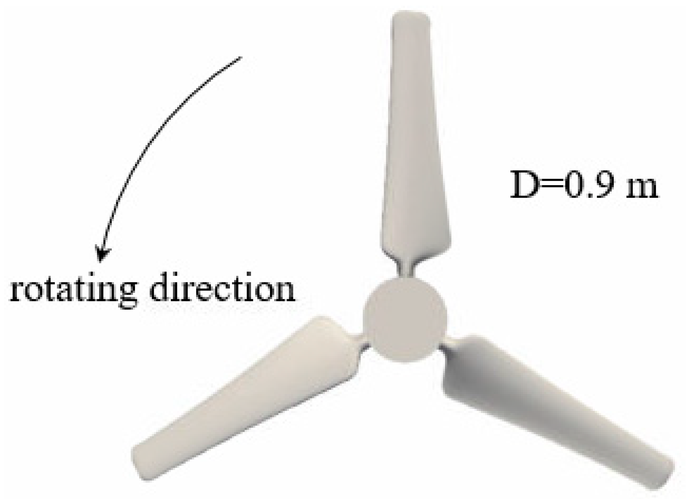
3.1. Baseline Model and Mesh Dependency Test

The baseline model of HATST [23] is as shown in Figure 2 and has a three-bladed HATST of a selected diameter of 0.9 m. The blades rotated counterclockwise. The NACA 63–418 hydrofoil section was used for the turbine blade. To maintain a uniform lift force generation in the spanwise direction, various twist angles of the hydrofoil section were applied in various spanwise positions [24].

The twist axis of each hydrofoil section was 1/4$C$ away from the leading edge. Here, $C$ is the chord length. No twist angle was applied at the hub fitting part. The TSR was set 3 to 8, and the designed freestream flow was 0.68 m/s. The Reynolds number based on the freestream flow was ranged from $6.6\times {10}^5$ to $2\times {10}^6$. The TSR was varied by changing the rotational speed of the turbine in the present study. To set different TSRs, the inflow velocity was changed.

Since the mesh density substantially affected the accuracy of CFD simulations, there were strict requirements for mesh quality and count inside the AMI zone where the speed of flow was high. In addition, to accurately capture the wave elevation, the mesh around the free surface needed to be refined. A relatively sparse mesh was used in other regions to improve the computational efficiency.

The mesh dependency verification was performed to determine the optimal mesh count to predict the power performance and capture the flow features around the turbine. Three mesh types, Mesh-1, Mesh-2 and Mesh-3, were selected to demonstrate the mesh dependence attributed to different mesh densities, as shown in Figure 3. In the mesh dependency test, the present study was focused on the power coefficient. The meshes around the free surface were the same for all three meshes. The time step was also an important factor affecting the results. Therefore, the computations were performed at the time step of 0.0001 s, and the Courant numbers were not exceeded one during the simulations.

The test condition with TSR = 4.5, $U_{\infty }$ = 0.68 m/s, wave frequency $f$ = 0.7 Hz and amplitude $A$ = 80 mm was selected. The power coefficients for three unstructured meshes are listed in

Table 1. Mesh dependency test results.

	Mesh Count	${\mathit{C}}_{\mathit{p}}$	$\mathbf{Difference} \mathbf{of} {\mathit{C}}_{\mathit{p}}$
Mesh-1 ($N_1$)	856,223	0.290938	29.09%
Mesh-2 ($N_2$)	1,662,963	0.408875	0.69%
Mesh-3 ($N_3$)	2,502,535	0.411691

. The used mesh count of Mesh-1 ($N_1$), Mesh-2 ($N_2$) and Mesh-3 ($N_3$) were 856,223, 1,662,963 and 2,502,535, respectively. The difference of the power coefficient for Mesh-1 ($N_1$) was calculated by $\frac{N_2-N_1}{N_1}\times 100 \left(\%\right)$. The power coefficients on the target blade obtained from two simulations with Mesh-2 and Mesh-3 were very close, indicating that increasing the number of meshes had little effect on the computational convergence once the number of meshes reached a certain density. Therefore, considering the computational efficiency, Mesh-2 was chosen for the present simulations.

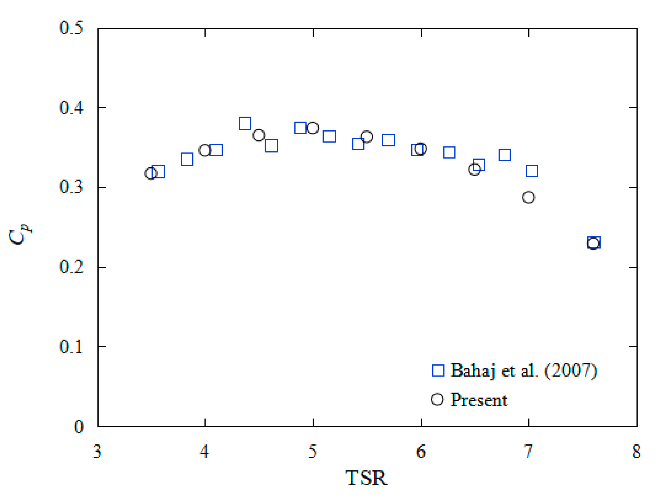
3.2. Power with Current-Only Case

To verify the numerical methods, the test condition for the HATST with the current only was selected [6]. The free surface was not considered. A three-bladed turbine with a 0.8 m diameter was used in the experiment. The blade shape was designed with 17 hydrofoil sections in the spanwise direction. The experiments were carried out in a 2.4 m × 1.2 m cavitation tunnel. The dimensions of the turbine and incoming velocity of 1.54 m/s were similar for both the experiments [6] and the present simulations. The power coefficients were obtained by changing the inflow velocities. The comparison of the present and experimental results for various TSRs is shown in Figure 4. The power coefficient for various TSRs of the present CFD results showed a similar trend as the experimental data [6].

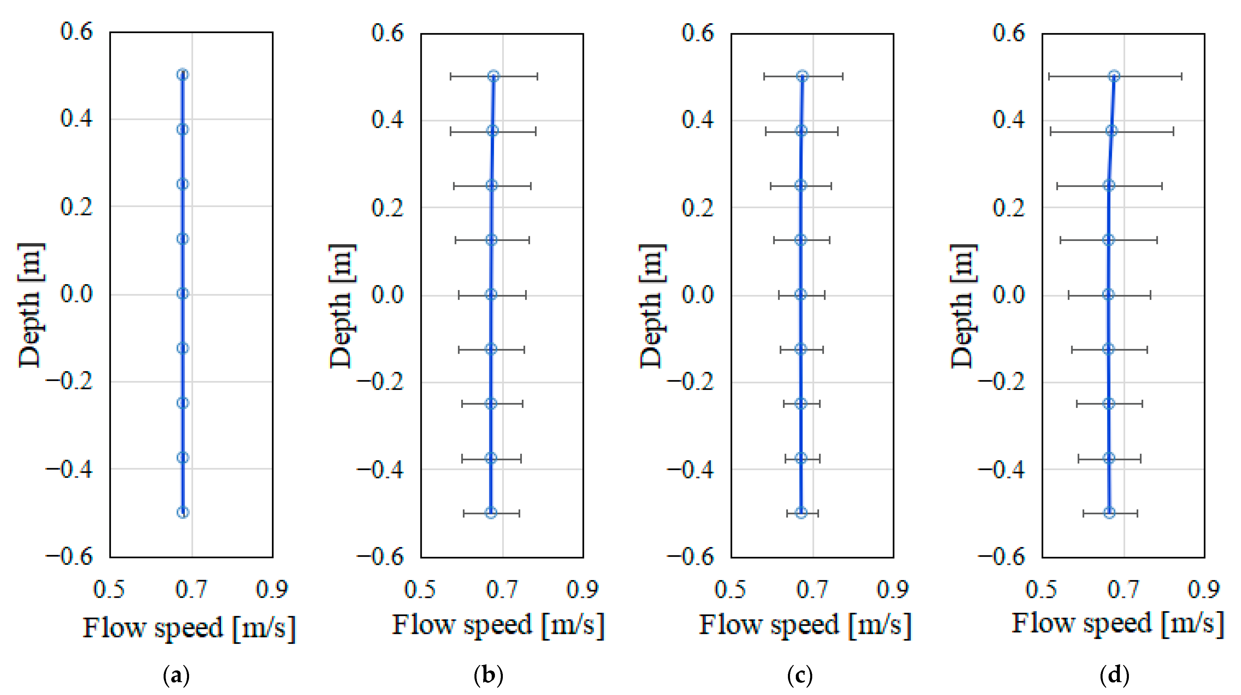
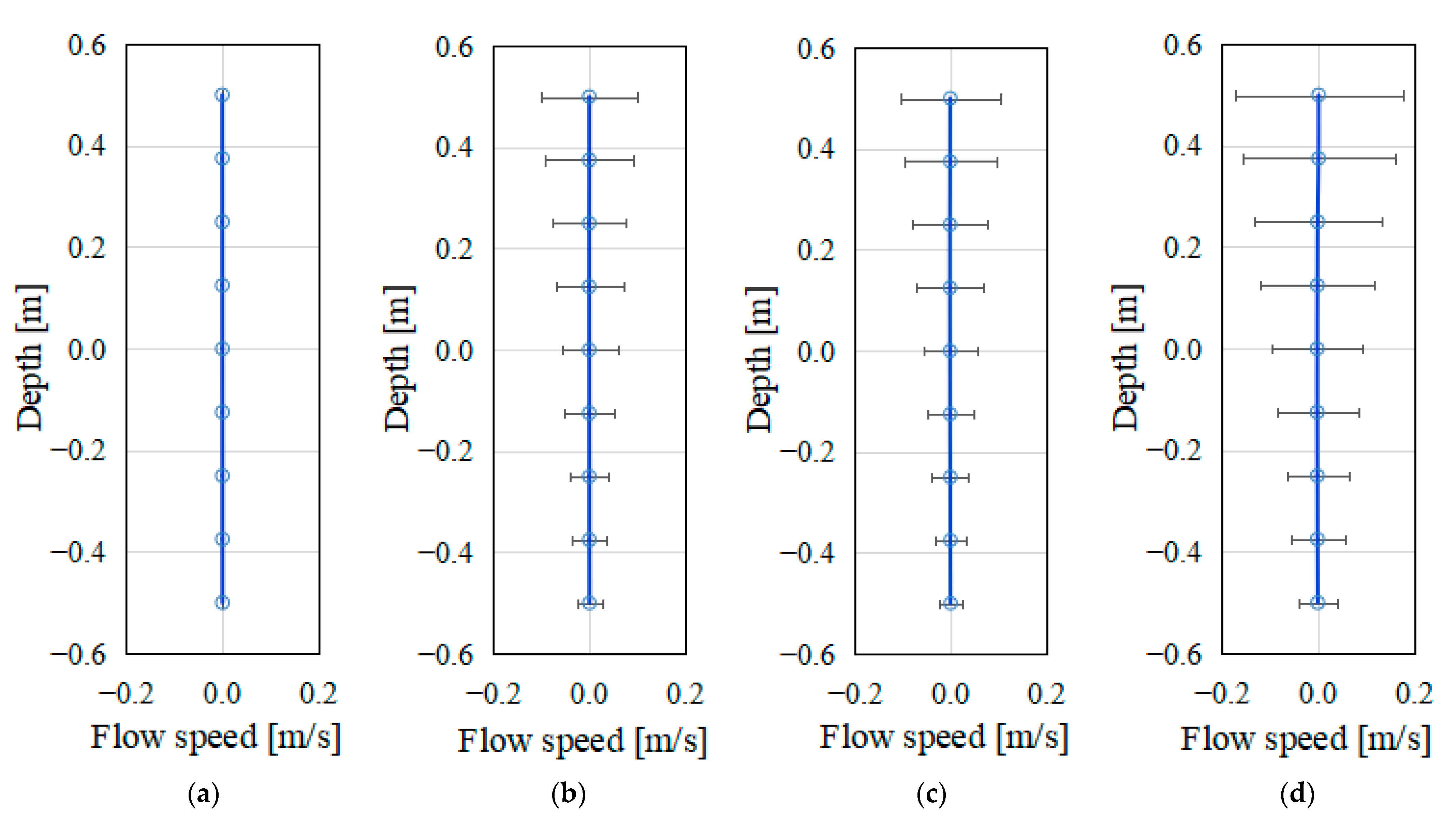
3.3. Wave Generation in Current

The wave and current without the turbine were considered. To generate the waves and currents, a third-order Stokes theory was used, which was more consistent with the actual wave. The current of $U_{\infty }$= 0.68 m/s and the wave of $f$ = 0.7 Hz and $A$ = 80 mm were considered at the inlet boundary. The profile of the generated wave was compared with that of the third-order Stokes wave theory. The computational domain size was same for the turbine simulation cases. The converged wave profile was obtained after two wavelengths. The comparison between the present and the theory is shown in Figure 5. The wave profile was captured above the turbine center at different times. After the numerical stabilization of the waves, the root mean square error (RMSE) between the theoretical data and present results was 0.0071. The present results were similar to the theoretical results, which verified the accuracy and feasibility of the simulations of the wave and current [25]. The present results demonstrated a satisfactory agreement with the theoretical results, indicating that the feasibility and accuracy of the wave and current simulations were verified.

4. Results and Discussion

To study the wave effects on the incoming flow speed to the turbine, the axial and vertical velocities around the turbine were investigated. The wave and current conditions considered are listed in

Table 2. Test conditions for wave and current interactions.

	Current (m/s)	Wave Frequency (Hz)	Wave Amplitude (m)
Case 1	0.68	-	-
Case 2	0.68	0.5	0.08
Case 3	0.68	0.7	0.08
Case 4	0.68	0.7	0.14

. To study the effect of the wave frequency, Cases 2 and 3 were selected. Cases 3 and 4 were considered for the wave amplitude effect.

Figure 6 and Figure 7 showed the averaged axial and vertical velocities at the turbine’s location. The hub of the turbine was located at z = 0. The axial mean velocity decreased slightly due to the waves. The vertical mean velocity was virtually unaffected by the waves. The closer to the free surface, the greater the range of variation of the axial and vertical velocities. The effect of the wave amplitude was more pronounced, while different wave frequencies had less effect on the axial and vertical velocities. Increasing the wave frequency resulted in a larger fluctuation away from the free surface.

The turbine’s performance under the waves and currents was studied. The power coefficients obtained from the current of $U_{\infty }$ = 0.68 m/s and the wave of $f$ = 0.7 Hz and $A$ = 80 mm were compared with the experimental data [23] (Figure 8). The power coefficients for various TSRs are shown in Figure 4. The power coefficients used were the mean value due to the wave. The present CFD results were consistent with the experimental data, confirming that the selected numerical methods could predict the performance of the turbine quite accurately. The maximum power coefficient was observed at TSR = 4.5 under the waves and currents.

The effect of the waves on the turbine was studied because the axial component of the incoming flow was varied due to the waves. As shown in Figure 9, it was investigated for the wave crest (①), down-crossing (②), trough (③), and up-crossing (④) according to the wave profile located on the turbine.

Figure 10 shows the axial velocity contours with different wave phases around the turbine. The axial velocity was nondimensionalized by the incoming current velocity. The current of $U_{\infty }$= 0.68 m/s with TSR = 4.5 and the wave of $f$ = 0.7 Hz and $A$ = 80 mm were considered. The power coefficient had the maximum value at TSR = 4.5. When the wave crest passed through the turbine, a high velocity was observed; however, when the wave trough passed, a low velocity was observed. At the wave up-crossing and down-crossing, the velocities were almost the same and were in range of the velocities at the wave crest and trough.

Table 3. Power coefficients for various wave elevations.

Wave	Crest (①)	Down-Crossing (②)	Trough (③)	Up-Crossing (④)
Cp	0.545	0.397	0.264	0.401

lists the power coefficients for various wave elevations on the turbine. The power coefficients were varied with the wave elevation. Figure 11 shows the vortical flow with the iso-surface of Q-criterion = 0.1 behind the turbine. The Q-criterion indicated the areas where the magnitude of vorticity was larger than the magnitude of the strain rate. The Q-criterion is usually used to visualize the vortices. The vortices were colored based on the axial velocity. A vortical flow separation was observed at the tip of the blades and strong vortices were shedding at the wave crest. The vortices gradually appeared outward along the center of the turbine due to a fast flow velocity. The vortical flows generated at the tip were diffused in different directions. The tip vortices propagated upward at the wave crest and downward at the wave trough. The vortical flows with the same radius were observed at the wave down-crossing and up-crossing. The strength of the vortices was proportional to the wave height. Small vortices around the trailing edge were observed.

The effect of various wave frequencies and heights was studied. Figure 12 shows the nondimensionalized axial velocity contours around the turbine at x = 0 at the wave crest. The flow around the turbine was accelerated due to the wave crests. The effect of the wave amplitudes was significant, while the effect of the wave frequency was insignificant. It was observed that velocities around the free surface were higher than elsewhere.

Table 4. Maximum power coefficients for various wave conditions.

	Case 1	Case 2	Case 3	Case 4
$C_p$	0.437	0.608	0.549	0.655

lists the maximum power coefficients at the wave crest. The maximum power coefficients at the wave crest were larger than that without the waves. The wave height had a great impact on the power coefficient. Figure 13 shows the vortical flow with the iso-surface of Q-criterion = 0.1 behind the turbine at the wave crest. The large wave height created a strong vortical flow. Moreover, the increased wave amplitude changed the shape of the vortical flow structure, while the increased wave frequency only affected the velocity magnitude. The difference in wave height had a significant effect on the axial velocity and strong vortices.

Figure 14 shows the nondimensionalized axial velocity contours around the turbine at the wave trough. The flow around the turbine was decelerated due to the wave troughs. The effect of the wave heights was significant, whereas the effect of the wave frequency was insignificant.

Table 5. Minimum power coefficients for various wave conditions.

	Case 1	Case 2	Case 3	Case 4
$C_p$	0.437	0.214	0.261	0.156

lists the minimum power coefficients at the wave trough. The minimum power coefficients at the wave trough were smaller than that without the waves. Due to the large wave trough, Case 4 showed the minimum power coefficient. Figure 15 shows the vortical flow with the iso-surfaces of Q-criterion = 0.1 behind the turbine at the wave trough. The low wave trough created a weak vortical flow. The changing wave height had significant effects on the incoming velocity to the turbine. Varying the wave elevation affected the incoming velocity and vortical flow strength, indicating that there could be a resultant fatigue on the turbine blade.

For the current of $U_{\infty }$ = 0.68 m/s and the wave of $f$ = 0.7 Hz and $A$ = 80 mm, the relation between the wave elevation and power coefficient is shown in Figure 16. The power coefficient was varied according to the wave elevation. The power of HATST had the maximum and minimum values at the wave crest and trough, respectively.

5. Concluding Remarks

CFD simulations were applied to predict the power performance and flow characteristics of the HATST, taking into account the interaction of waves and currents. To simulate the two-phase fluid flow, OpenFOAM, which is an open source CFD library platform, was used. Mesh dependency tests were performed and the converged results with the medium and fine meshes were obtained. To improve the computational efficiency, the medium mesh was selected for the present studies. The prediction considered the power performance of the turbine under only the current. The power coefficient under only the current showed a similar tendency as the experimental data [6]. To accurately predict the waves and currents, Olaflow [16] based on the OpenFOAM platform was used. The generated wave with the current was compared with the Stokes third-wave theory. It was confirmed that the selected mesh could simulate the wave and current together well.

To study the effect of waves on the turbine performance, different wave frequencies and amplitudes were considered. The power coefficient varied with the wave elevation under waves and currents. The power coefficient reached its maximum and minimum values at the wave crest and trough, respectively. The vortical flow was generated at the blade tip of the turbine. The wave crest caused a strong vortical flow, while the wave trough caused a weak vortical flow. The wave elevation could affect the radius of the vortical flow. The radius of the vortical flow behind the turbine was increased at the wave crest and decreased at the wave trough. At the wave up-crossing and down-crossing, the radius of the vortical flow was kept constant. It was confirmed that the wave elevation could affect the radius of the vortical flow. The effect of the wave amplitude on the turbine’s performance was larger than that of the wave frequency. Because the periodic power change due to the varying wave amplitude can cause the vibration and fatigue failure of turbines in the long term, an in-depth research is required.

In summary, it is necessary to consider the effect of waves and currents in the design of HATSTs. The proposed numerical methods could provide a reference for the design of HATSTs under the waves and currents. Blade deformation due to varying wave elevation will be studied in future works.

References

1. Alipour, R.; Alipour, R.; Fardian, F.; Tahan, M.H. Optimum performance of a horizontal axis tidal current turbine A numerical parametric study and experimental validation. Energy Convers. Manag. 2022, 258, 115533. [Google Scholar] [CrossRef]
2. Afgan, I.; McNaughton, J.; Rolfo, S.; Apsley, D.D.; Stallard, T.; Stansby, P. Turbulent flow and loading on a tidal stream turbine by LES and RANS. Int. J. Heat Fluid Flow 2013, 43, 96–108. [Google Scholar] [CrossRef]
3. Tian, W.; Mao, Z.; Ding, H. Design, test and numerical simulation of a low-speed horizontal axis hydrokinetic turbine. Int. J. Nav. Archit. Ocean Eng. 2018, 10, 782–793. [Google Scholar] [CrossRef]
4. Marsh, P.; Ranmuthugala, D.; Penesis, I.; Thomas, G. Three-dimensional numerical simulations of straight-bladed vertical axis tidal turbines investigating power output, torque ripple and mounting forces. Renew. Energy 2015, 83, 67–77. [Google Scholar] [CrossRef] [Green Version]
5. Ng, K.W.; Lam, W.H.; Ng, K.C. 2002–2012: 10 Years of Research Progress in Horizontal-Axis Marine Current Turbines. Energies 2013, 6, 1479–1526. [Google Scholar] [CrossRef] [Green Version]
6. Bahaj, A.S.; Molland, A.F.; Chaplin, J.R.; Batten, W.M.J. Power and thrust measurements of marine current turbines under various hydrodynamic flow conditions in a cavitation tunnel and a towing tank. Renew. Energy 2007, 32, 407–426. [Google Scholar] [CrossRef]
7. Barltrop, N.; Varyani, K.S.; Grant, A.; Clelland, D.; Pham, X.P. Investigation into wave-current interactions in marine current turbines. SAGE J. 2006, 221, 233–242. [Google Scholar] [CrossRef]
8. Fernandez-Rodriguez, E.; Stallard, T.J.; Stansby, P.K. Experimental study of extreme thrust on a tidal stream rotor due to turbulent flow and with opposing waves. J. Fluids Struct. 2014, 51, 354–361. [Google Scholar] [CrossRef]
9. Kinnas, S.A.; Xu, W.; Yu, Y.H.; He, L. Computational methods for the design and prediction of performance of tidal turbines. J. Offshore Mech. Arct. Eng. 2012, 134, 11101. [Google Scholar] [CrossRef]
10. Harrison, M.E.; Batten, W.M.J.; Myers, L.E.; Bahaj, A.S. Comparison between CFD simulations and experiments for predicting the far wake of horizontal axis tidal turbines. IET Renew. Power Gener. 2010, 4, 613–627. [Google Scholar] [CrossRef]
11. Lee, S.H.; Lee, S.H.; Jang, K.; Lee, J.; Hur, N. A numerical study for the optimal arrangement of ocean current turbine generators in the ocean current power parks. Curr. Appl. Phys. 2010, 10, 137–141. [Google Scholar] [CrossRef]
12. Park, S.; Park, S.; Rhee, S.H. Influence of blade deformation and yawed inflow on performance of a horizontal axis tidal stream turbine. Renew. Energy 2016, 92, 321–332. [Google Scholar] [CrossRef]
13. Tian, W.; Ni, X.; Mao, Z.; Zhang, T. Influence of surface waves on the hydrodynamic performance of a horizontal axis ocean current turbine. Renew. Energy 2020, 158, 37–48. [Google Scholar] [CrossRef]
14. Tatum, S.C.; Frost, C.H.; Allmark, M.; Doherty, D.M.O.; Mason-Jones, A.; Prickett, P.W.; Grosvenor, R.I. Wave-current interaction effects on tidal stream turbine performance and loading characteristics. Int. J. Mar. Energy 2016, 14, 161–179. [Google Scholar] [CrossRef] [Green Version]
15. Zhang, Z.; Zhang, Y.Q.; Zheng, Y.; Zhang, J.S.; Emmanuel, F.R.; Zang, W.; Ji, R.W. Power fluctuation and wake characteristics of tidal stream turbine subjected to wave and current interaction. Energy 2023, 264, 126185. [Google Scholar] [CrossRef]
16. Higuera, P. Enhancing active wave absorption in RANS models. Appl. Ocean Res. 2020, 94, 102000. [Google Scholar] [CrossRef]
17. Frank, M.W. Viscous Fluid Flow, 3rd ed.; McGraw-Hill Education: New York, NY, USA, 2006. [Google Scholar]
18. Damián, M. An Extended Mixture Model for the Simultaneous Treatment of Short and Long Scale Interfaces. Ph.D. Thesis, Universidad Nacional del Litoral, Santa Fe, Argentina, 2013. [Google Scholar]
19. Umeyama, M. Coupled PIV and PTV Measurements of Particle Velocities and Trajectories for Surface Waves Following a Steady Current. J. Waterw. Port Coast. Ocean Eng. 2011, 137, 85–94. [Google Scholar] [CrossRef]
20. Crank, J.; Nicolson, P. A practical method for numerical evaluation of solutions of partial differential equations of the heat-conduction type. Adv. Comput. Math. 1996, 6, 207–226. [Google Scholar] [CrossRef]
21. Menter, F.R. Two-equation eddy-viscosity turbulence models for engineering applications. AIAA J. 1994, 32, 1598–1605. [Google Scholar] [CrossRef] [Green Version]
22. Park, S.; Park, S.; Rhee, S.H.; Lee, S.B.; Choi, J.E.; Kang, S.H. Investigation on the wall function implementation for the prediction of ship resistance. Int. J. Nav. Archit. Ocean Eng. 2013, 5, 33–46. [Google Scholar] [CrossRef]
23. Gaurier, B.; Davies, P.; Deuff, A.; Germain, G. Flume tank characterization of marine current turbine blade behaviour under current and wave loading. Renew. Energy 2013, 59, 1–12. [Google Scholar] [CrossRef] [Green Version]
24. Gaurier, B.; Germain, G.; Facq, J.; Bacchetti, T. Three tidal turbines in interaction: An experimental study of turbulence intensity effects on wakes and turbine performance. Renew. Energy 2020, 148, 1150–1164. [Google Scholar] [CrossRef]
25. Wang, S.; Li, C.; Zhang, Y.; Zhang, T. Influence of pitching motion on the hydrodynamic performance of a horizontal axis tidal turbine considering the surface wave. Renew. Energy 2022, 189, 1020–1032. [Google Scholar] [CrossRef]
Figure 1. Boundary conditions and computational domain extent: (a) Schematic; (b) simulation.
Jmse 11 00425 g001
Figure 2. Three-bladed baseline turbine model with rotating direction.
Jmse 11 00425 g002
Figure 3. Three typical meshes: (a) Mesh-1; (b) Mesh-2; (c) Mesh-3.
Jmse 11 00425 g003
Figure 4. Power coefficient under current [6].
Jmse 11 00425 g004
Figure 5. Comparison of wave elevation for present and theory.
Jmse 11 00425 g005
Figure 6. Axial averaged and variation range under waves and currents: (a) Case 1; (b) Case 2; (c) Case 3; (d) Case 4.
Jmse 11 00425 g006
Figure 7. Vertical averaged and variation range under waves and currents: (a) Case 1; (b) Case 2; (c) Case 3; (d) Case 4.
Jmse 11 00425 g007
Figure 8. Power coefficient under waves and currents [23].
Jmse 11 00425 g008
Figure 9. Different wave phases on the turbine.
Jmse 11 00425 g009
Figure 10. Axial velocity contours around the turbine for various wave elevations: (a) crest; (b) down-crossing; (c) trough; (d) up-crossing.
Jmse 11 00425 g010
Figure 11. Vortical flow with iso-surfaces of Q = 0.1 for various wave elevations: (a) crest; (b) down-crossing; (c) trough; (d) up-crossing.
Jmse 11 00425 g011
Figure 12. Axial velocity contours around the turbine at wave crest of different wave conditions: (a) Case 1; (b) Case 2; (c) Case 3; (d) Case 4.
Jmse 11 00425 g012
Figure 13. Vortical flow with iso-surfaces of Q = 0.1 at wave crest of different wave conditions: (a) Case 1; (b) Case 2; (c) Case 3; (d) Case 4.
Jmse 11 00425 g013
Figure 14. Axial velocity contours around the turbine at wave trough of different wave conditions: (a) Case 1; (b) Case 2; (c) Case 3; (d) Case 4.
Jmse 11 00425 g014
Figure 15. Vortical flow with iso-surfaces of Q = 0.1 at wave trough of different wave conditions: (a) Case 1; (b) Case 2; (c) Case 3; (d) Case 4.
Jmse 11 00425 g015
Figure 16. Relation of wave elevation and power coefficient.
Jmse 11 00425 g016