Sensitivity Analysis of Ship Manoeuvring Mathematical Models

Abstract

Sensitivity analysis is applied to ship manoeuvring mathematical models as a means of dealing with model uncertainties, and often leads to model simplifications. A rather standard 3DOF manoeuvring model was tuned with the available results of full-scale trials of a naval combatant and was further used as the reference model for sensitivity analysis. The present research was based on multiple perturbed simulations of the turning, zigzag and spiral manoeuvres. A salient feature of the present study is that the perturbations were applied to the total hydrodynamic forces and moments as well as separately to their characteristic parts, i.e., to the linear and nonlinear single-variable and coupled components. Another special feature is that the deviations of the perturbated responses were estimated not only considering the standard manoeuvring performance indices, but also through application of the Euclidean metric directly to the time histories and to the spiral curve. The performed analysis permitted the sensitivity of the model to be traced to various parameters and groups thereof. It was established that the highest sensitivity of the model was to linear and some nonlinear multivariable parameters, and the Euclidean metric permitted a more detailed analysis than that based only on standard discrete manoeuvring indices. The obtained results are expected to be useful in the application of system identification methods to typical inherently stable fast surface-displacement ships.

1. Introduction

Ship manoeuvring mathematical models are an important part of all existing bridge and desktop manoeuvring simulators. As these simulators must provide high simulation speeds in real or accelerated time and must also guarantee good realism of simulations, the models used must represent a compromise between complexity and effectiveness [1,2]. This requirement precludes the use of in-the-loop CFD computations to simulate the manoeuvring forces. Instead, much faster holistic or modular models based on ordinary differential equations depending on a limited number of parameters are applied. The values of these parameters must be specified to assure acceptable adequacy of the simulation [3,4]. However, there is always uncertainty associated with these manoeuvring models, both arising from external factors and inherent to the mathematical model. This jeopardises the accuracy of the simulated responses and trajectories based on such models [5]. The uncertainty associated with the initial conditions of the ship was addressed in [6], but it is also important to analyse the effect of the uncertainty of the manoeuvring model and its coefficients.

To reduce the uncertainty of a model, offline CFD computations [7] or physical captive-model tests [8] can be used, but the obtained values of the parameters of the model must typically be adjusted or tuned, either manually or using system identification often based on full-scale trials. In any case, the uncertainty of the model depends on its sensitivity to variations in its parameters [9,10]. These facts triggered the interest in performing the present sensitivity studies.

This work contributes to the general effort developed by the ISSC-ITTC Joint Committee on Uncertainty Modelling, which is promoting the further development of methods of uncertainty modelling of waves [11,12] and ship responses [13,14].

The sensitivity analysis studies on manoeuvring may have started with Hwang [15,16], who performed a sensitivity analysis within the process of system identification of a 3DOF mathematical model modelling the OSAKA super tanker, applying the so-called indirect method to zigzag and turning circle manoeuvres.

In the indirect method, one runs the reference model and saves the results $y_i\left({\theta }_0\right)$, then changes one model parameter by a certain amount $\Delta {\theta }_j$, reruns the mathematical model and saves the corresponding results $y_i\left({\theta }_j+\Delta {\theta }_j\right)$. The goal of calculating the sensitivity of model parameters is to determine the ratio between the relative changes of the model parameters and the model output [17,18], as shown in

$$S_i^j=\frac{\partial y_i}{\partial {\theta }_j}\approx \frac{y_i\left({\theta }_j+\Delta {\theta }_j\right)-y_i\left({\theta }_j\right)}{\Delta {\theta }_j}$$

(1)

where $S_i^j$ is a measure of sensitivity, $y_i$ is the $i\mathrm{th}$ motion parameter and ${\theta }_j$ is the $j\mathrm{th}$ mathematical model coefficient. The measure of sensitivity is based on the maximum distance between the values of the reference output parameters and those obtained by a 20% perturbation of the input parameters. It has been found that the linear coefficients are always important, and the inertia terms and the nonlinear coefficients play a more important role in tight manoeuvres. The yaw force and moment due to the rudder angle become more influential when the manoeuvre is tighter. The yaw moments due to sway and yaw velocities exchange relevance from moderate to tight manoeuvres.

Kose and Misiag [19,20] studied the sensitivity of a modular mathematical model belonging to the so-called MMG family to variations in its parameters. They aimed to find the parameters that most affected the estimation of the manoeuvring performance, namely the hull added mass coefficients, the linear manoeuvring derivatives and some interaction parameters for the rudder and propeller. Using the indirect method, they studied the effects of variation of these parameters on zigzag and turning manoeuvres. The disturbed parameters were treated as Gaussian random numbers, having the mean as a reference value and six levels of standard deviation, from 1 to 25 percent of the reference value. This study showed that the most influencing parameters were the linear manoeuvring derivatives and the least influencing were the added mass coefficients.

Ishiguro et al. [21], using the indirect method, performed a sensitivity analysis on the simulation parameters of an MMG mathematical model applied to different hull forms. The authors were looking for the parameters that should be considered at the early design stage for more accurate results on the prediction of a ship’s manoeuvrability. Therefore, they performed a sensitivity study wherein the simulation parameters were categorised into linear hydrodynamic derivatives, nonlinear hydrodynamic derivatives, interaction coefficients and inertial coefficients. The manoeuvres used for the study were the turning circle and zigzag. Sensitivity was measured as “relative sensitivity”: the ratio of change in the results when each parameter is individually increased by 10%. This value is 1.0 when the output parameter increases by 10% as a result of a 10% increase in an input parameter. They concluded that almost every linear hydrodynamic derivative significantly affected the predicted results. These sensitivities became higher when the degree of directional stability was reduced.

Rhee and Kim [22] performed a sensitivity analysis on an MMG mathematical model of the Esso Osaka. The sensitivity analysis was performed to clarify the effect of each input parameter on the system before performing system identification. It was argued that if there is no effect of a coefficient on the system, it is nearly impossible to estimate it; mutatis mutandis, if a coefficient has a significant effect on the system, it is more identifiable. Using zigzag and turning manoeuvres, they concluded that linear coefficients had the highest influence on the model’s behaviour and that their influence diminished with tighter manoeuvres. The model showed lower sensitivity to nonlinear coefficients, but their influence increased with the steepness of the manoeuvre. It was also concluded that the higher the sensitivity, the higher the identification efficiency.

While the authors reviewed so far have made use of the indirect method of sensitivity analysis, Yeo and Rhee [17] proposed to use a direct method arguing that the indirect method implies that the number of required simulations increases together with the number of input parameters thus making generalization of the sensitivity analysis impossible. The direct method is more computationally demanding since it requires the differentiation of mathematical models with respect to the model coefficients. However, it shows the sensitivity history of the dynamic system during the manoeuvring simulation. Zigzag and turning circle manoeuvres were simulated and it was concluded that different hull geometries differently affected the sensitivity of the hydrodynamic coefficients, and the sensitivity was dependent on the type of manoeuvre.

Wang et al. [18] performed a sensitivity analysis using the direct method proposed by Yeo and Rhee [17], using a 4DOF mathematical model for a container ship. The aim was to reduce the number of hydrodynamic coefficients to be determined by employing system identification. The chosen performance parameters were the surge and sway velocities, rate of yaw and rate of roll. For the sensitivity calculation, they simulated one spiral manoeuvre. To decide which coefficients to keep in the mathematical model, minimum threshold values were defined for the total sensitivity value. The validity of the simplified model was verified by simulating a zigzag manoeuvre using the original and the simplified mathematical models.

Wang et al. [18] performed a sensitivity analysis using the indirect method on the 4DOF mathematical model developed by Pérez and Blank [23]. They argued that the direct method, while providing the sensitivity history in one run, is computationally very demanding, while the indirect method requires more runs but the computational effort and memory storage in each run are small. For the sensitivity calculation, they simulated an “S-type” manoeuvre. A sensitivity analysis was then performed by perturbing the reference parameters by 10% to 50%. The decision of which coefficients to keep in the mathematical model was based on minimum threshold values defined for the sensitivity indices, which varied from 0.045% to 0.145%. The validity of the simplified model was verified for simulating zigzag and turning manoeuvres using the original and the simplified mathematical models.

From this review, it can be seen that sensitivity analysis as a means of improving the efficiency of system identification or simplifying mathematical models while keeping the response as close as possible to real ship behaviour has been in practice in the manoeuvring research community since at least 1969 [15].

There are two approaches for implementing sensitivity analysis in manoeuvring: the direct method [17,24] and the indirect method [16,18,19,20,21]. Both methods yield similar trends in the sense that the “linear” derivatives have more influence than the “nonlinear” derivatives and the added mass coefficients, although the level of sensitivity changes depending on the manoeuvre and the hull configuration. The tighter the manoeuvre, the more sensitive the mathematical model is to the nonlinear coefficients. The direct method demands much more computational effort than the indirect method.

There is no standard metric and method for sensitivity analysis. However, any metric and method considered must account for the output parameters which are of interest and soundly show the sensitivity of these output parameters to the input parameters per type of manoeuvre.

Significant scientific research has been done to find reliable yet simplified mathematical models of manoeuvring using sensitivity analysis tools. However, there is still no provision for a common methodological ground for carrying out a sensitivity analysis or how to define a threshold to keep the relevant parameters and discard the remaining ones.

In most previous studies on the sensitivity of manoeuvring models, traditional manoeuvring indices, e.g., tactical diameter, advance and peak overshoots, were used to measure changes in the model’s response. Others inspected and analysed the plots of outputs directly [4]. In this study, the focus was on the application of the Euclidean metric directly to the time histories of selected kinematic parameters in three standard definitive manoeuvres. This approach represents some novelty in the field of manoeuvring studies, and it is possible that this measure of the variation of the output is more consistent, as the closeness of kinematic responses in the Euclidean sense infers closeness of traditional manoeuvrability measures while the opposite is not necessarily true.

The analysis was performed on a 3DOF frigate mathematical model. Besides the metric used in this investigation, it is believed from the review that the method used to perform the sensitivity analysis in this work is also new, with four output parameters and three manoeuvres in six variations: the turning manoeuvre with 10/20/30 deg helms, the zigzag manoeuvre at 10–10 and 20–20 deg and the spiral manoeuvre. The work provides evidence not only of the relevant hydrodynamic input parameters, but also of the relevance of each manoeuvre and its tightness. The study was performed in a pattern of deepening detail, simulating 420 manoeuvring runs, starting with total perturbations induced to the hydrodynamic forces in surge, sway and yaw, followed by partial and semipartial perturbations applied first to the linear regressors and then to the nonlinear uncoupled and coupled (mixed) regressors.

Section 2 of the present article includes a description of the methods used for the sensitivity analysis (Subsection 2.1), a detailed description of the reference ship mathematical model (Subsection 2.2) and an outline of all specifics related to the application of the sensitivity analysis to the ship mathematical model under consideration (Section 2.3, Section 2.4 and Section 2.5). The obtained numerical results and their discussion are located in Section 3. The final section of the article contains the conclusions.

2. Materials and Methods

2.1. Method of Sensitivity Analysis

This work intended to analyse the responses of the mathematical model to rather large (±50%) perturbations of its parameters. This level of perturbation is believed to be significant for an inherently directionally stable ship and is within the range referred to by Pérez and Blank [23] and Wang et al. [18]. The sensitivity analysis used the indirect method, which relies on running a reference simulation with unperturbed parameters followed by simulations with perturbed models. The SA did not explicitly include the level of uncertainty of the input parameters and its propagation to the output parameters in a global SA sense, as was performed by Silva and Guedes Soares [6], in whose study the mathematical model parameters were modelled as uncertain throughout the ship’s operational life due to the inherent stochastic variation of ship trim, draft and displacement.

The model’s behaviour was studied in deepening detail. First, the total perturbation of the external forces was performed, part of which, total perturbation without combinations, was previously developed and discussed by Silva et al. [25]. They concluded that the relevant forces in the turning manoeuvre and zigzag manoeuvre are the quasi-steady sway force and the yaw moment. The relevant forces in the outputs of the spiral manoeuvre are the sway force and, less clearly, the yaw moment.

This study further investigated the total perturbation with combinations and partial perturbation. Partial perturbation was applied first to the linear coefficients, then to the nonlinear single-variable coefficients and finally to the nonlinear multivariable coefficients. This approach itself is novel, to the best of our knowledge.

Several $k$ vectors of the output parameters ${\mathit{y}}_k$, ($k$ corresponding to the number of perturbed input parameters $\mathit{\theta }$) were considered. Each vector $\mathit{y}$ of length $N=T/\Delta t$, where $T$ is the time of simulation and $\Delta t$ is the timestep. Consider also that $n_M=6$ manoeuvres: $n_t=3$, $10°/20°/30°$ turning, $n_z=2$, $10°/20°$ zigzag and $n_s=1$, spiral. One possible sensitivity measure is the distance between two vector responses, i.e., the perturbed $\overline{\mathit{y}}={\left({\overline{y}}_1,\dots ,{\overline{y}}_N\right)}^T$ and the reference $\mathit{y}={\left(y_1,\dots ,y_N\right)}^T$ of equal dimension $N$, defined as follows:

$$\rho \left(\mathit{y},\overline{\mathit{y}}\right)={\sum }_{i=1}^N\rho \left(y_i,{\overline{y}}_i\right)$$

(2)

where $\rho \left(y_i,{\overline{y}}_i\right)$ is the metric for scalar responses. There are several options for choosing this metric in the functional space. Sutulo and Guedes Soares [26] tested the following metrics: the $L_1$ metric or absolute-value metric, the Euclidean or $L_2$ metric and the Hausdorff metric. The latter was demonstrated to be superior in the case of noisy responses. However, when the noise was absent, none of the tested metrics showed any tangible superiority. As no noise was present in this research, the most common Euclidean metric ${\rho }_E$ was preferred. It is defined as follows:

$${\rho }_E\left(y,\overline{y}\right)={\left[\underset{0}{\overset{T}{\int }}{\left(y\left(t\right)-\overline{y}\left(t\right)\right)}^{2}dt\right]}^{1/2}$$

(3)

where $t\in \left[0,T\right], T$ is the total duration of the simulation.

For the sensitivity analysis, an averaged $L_2$ metric over time was used as a “sensitivity index” $S$ to compare the effects of the $k\mathrm{th}$ perturbations. The discretised analogue to (3) was assumed in the following form:

$$\widetilde{L_2}={\left[\frac{{\sum }_{i=1}^N{\left(y\left(t_i\right)-\overline{y}\left(t_i\right)\right)}^2}{N}\right]}^{1/2}$$

(4)

It can be easily noticed that (4) is not quite equivalent to (3), as the latter is not multiplied by the duration time $T$; however, this is neither essential nor desirable for comparative studies where the $L_2$ metric of the $i\mathrm{th}$ kinematic parameter relative to the $j\mathrm{th}$ coefficient would be affected by the simulation duration, as is the case for the Z-manoeuvre. At the same time, dependence on the number of samples is removed.

2.2. Manoeuvring Mathematical Model

For the present work, a 3DOF nonlinear model was used, namely the standard Euler system of equations for a ship considered as a rigid body moving in the horizontal plane, in the following form:

$$\left(m+{\mu }_{11}\right)\dot{u}-mvr-m{x}_g{r}^2=X_q+X_p,$$

$$\left(m+{\mu }_{22}\right)\dot{v}+\left(m{x}_g+{\mu }_{26}\right)\dot{r}+mur=Y_q,$$

(5)

$$\left(m{x}_g+{\mu }_{62}\right)\dot{v}+\left(I_{zz}+{\mu }_{66}\right)\dot{r}+m{x}_{g}ur=N_q,$$

where $u$ is the surge velocity, $v$ is the sway velocity and $r$ is the yaw rate; the dotted variables are the corresponding accelerations, $m$ is the ship mass and ${\mu }_{ij}$ are the added mass coefficients. The forces on the hull due to the rudder are grouped as quasi-steady hydrodynamic forces (subscript q) on the hull and rudder in surge, sway and yaw, respectively. $X_p$ is the surge force exerted by the propeller (effective thrust). The forces may be represented as follows:

$$X_q={X^{\prime }}_q\left(u^{\prime },v^{\prime },{\delta }_R\right)\frac{\rho V^2}{2}LT,$$

$$Y_q={Y^{\prime }}_q\left(u^{\prime },v^{\prime },{\delta }_R\right)\frac{\rho V^2}{2}LT,$$

(6)

$$N_q=N{\prime }_q\left(u^{\prime },v^{\prime },{\delta }_R\right)\frac{\rho V^2}{2}{L}^{2}T,$$

where $X{\prime }_q$, $Y{\prime }_q$ and $N{\prime }_q$ are the dimensionless force or moment coefficients, $\rho$ is the water density, $V^2=u^2+v^2$ is the squared instantaneous ship speed, $L$ is the length of the ship and $T$ is the draught amidships.

The quasi-steady forces on Equations (5) and (6) are modelled as multivariate third-order regression polynomials depending on the nondimensional velocity components and rudder angle, with some terms dropped as insignificant.

$$\begin{array}{ll}X{\prime }_q=& X{\prime }_{uu}{u}^{\prime 2}+X{\prime }_{vr}{v}^{\prime }{r}^{\prime }+X{\prime }_{\delta \delta }{\delta }_R^2\\ Y{\prime }_q=& Y{\prime }_v{v}^{\prime }+Y{\prime }_{r}r\prime +Y{\prime }_{vvv}v{\prime }^3+Y{\prime }_{vvr}v{\prime }^2{r}^{\prime }+Y{\prime }_{\delta }{\delta }_R^{}+Y{\prime }_{\delta vv}v{\prime }^2{\delta }_R^{}+Y{\prime }_{\delta \delta v}v\prime {\delta }_R^2+\\ & Y{\prime }_{\delta \delta \delta }{\delta }_R^3\\ N{\prime }_q=& N{\prime }_v{v}^{\prime }+N{\prime }_{r}r+N{\prime }_{vvv}v{\prime }^3+N{\prime }_{vvr}v{\prime }^2{r}^{\prime }+N{\prime }_{\delta }{\delta }_R^{}+N{\prime }_{\delta vv}v{\prime }^2{\delta }_R^{}+\\ & N{\prime }_{\delta \delta v}{v}^{\prime }{\delta }_R^2+N{\prime }_{\delta \delta \delta }{\delta }_R^3\end{array}$$

(7)

where $X{\prime }_{uu}$ … $N{\prime }_{\delta \delta \delta }$ are the regression coefficients and ${\delta }_{\mathrm{R}}^{}$ is the rudder angle; $u^{\prime }$, $v^{\prime }$ and $r^{\prime }$ are the nondimensional velocity components, defined as

$$u^{\prime }=\frac{u}{V}; v^{\prime }=\frac{v}{V}; r^{\prime }=\frac{rL}{V}.$$

(8)

A first-order nonlinear model was used for the steering gear in the form proposed by Sutulo and Guedes Soares [27]. The coefficients in the model, the constant parameters and the propeller force model were as defined in [26]. The propulsion model for the propeller surge force was based on that described by the four-quadrant model proposed by Oltmann and Sharma [28] but adjusted using the procedure described in [29].

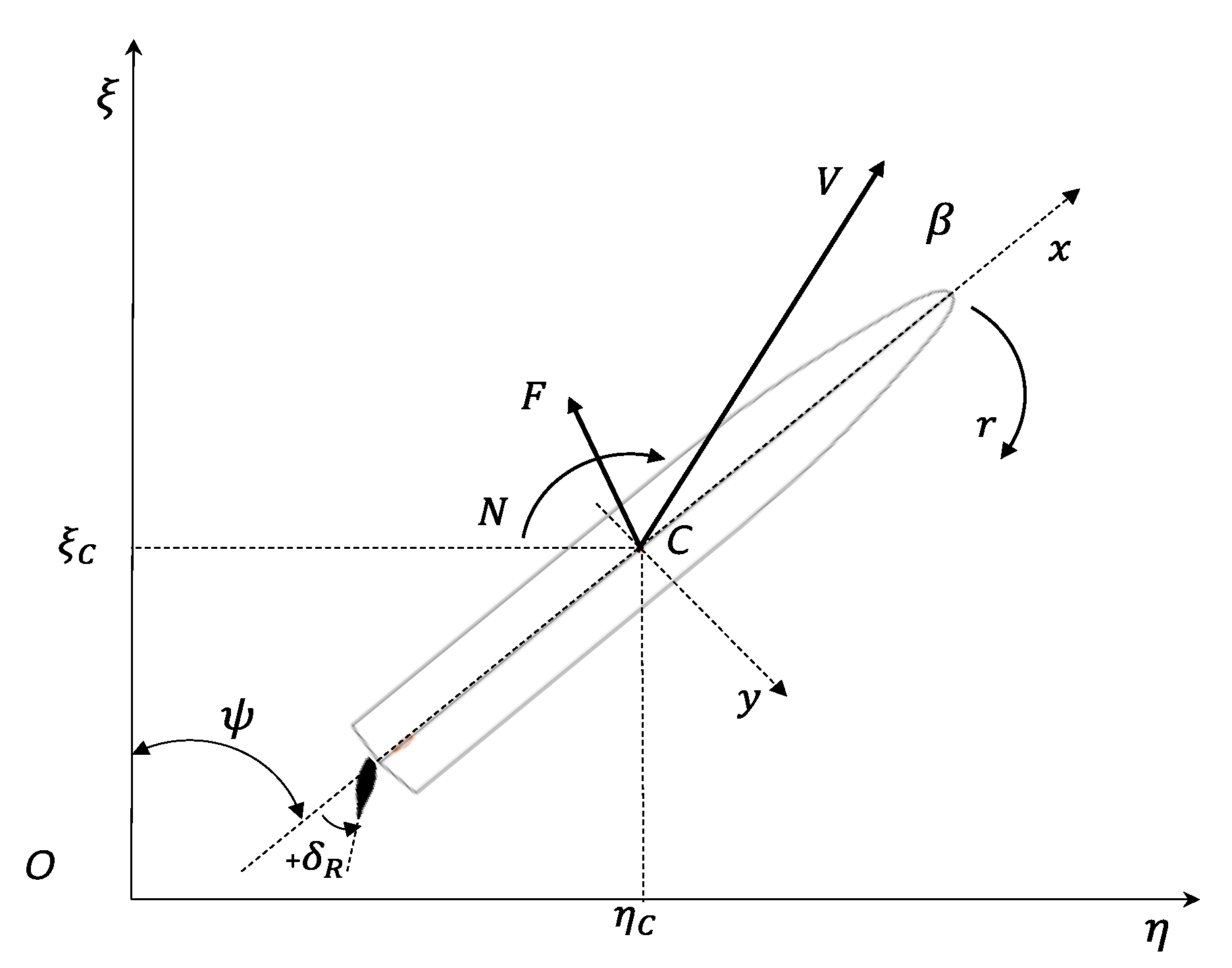
In general, this mathematical model can be viewed as half-modular, i.e., holistic for the hull–rudder system but with a separate submodel for the propeller. The model expressed in Equation (5) was extended with the kinematic equations needed for the transformation of the velocity components from the ship coordinate frame to the earth coordinate frame, given as

$$\begin{gathered} \dot{\xi }=u \cos \psi -v \sin \psi , \\ \dot{\eta }=u \sin \psi +v \cos \psi \end{gathered}$$

(9)

with the positive senses as presented in Figure 1.

The ship used as a case study to demonstrate the application of the method has a length between perpendiculars of 110m, a maximum beam of 13.8m, a draught of 4.1m and a mass of 3200 tonnes. The block coefficient is 0.505. The properties of mass/inertia are as follows: $I_{zz}=2.475\times {10}^9 \mathrm{kg}{m}^2, {\mu }_{11}=6.407\times {10}^4 \mathrm{kg}$, ${\mu }_{22}=1.896\times {10}^6$ kg, ${\mu }_{26}={\mu }_{62 }=-7.30\times {10}^6\mathrm{kg}{m}^2$, ${\mu }_{66}=1.199\times {10}^9 \mathrm{kg}{m}^2$. The nominal approach speed is $V_0=7.97$ m/s. Unfortunately, because of confidentiality issues, it is not possible to provide the body plan of the ship, but the hull shape is qualitatively typical of a frigate or destroyer-class surface-displacement ship. It has a transom stern and a large aft cut-off with a streamlined stabilising skeg. The propulsion-and-steering arrangement is also classic and includes two open screw propellers with a single rudder between them.

Table 1. Manoeuvring model coefficients for the ship under analysis.

Force/Moment DOF	Coefficient Value
$X$	$X{\prime }_{uu}$	$X{\prime }_{vr}$	$X{\prime }_{\delta \delta }$
	$-0.0091$	$-0.483$	$-0.0142$
$Y$	$Y{\prime }_v$	$Y{\prime }_r$	$Y{\prime }_{\delta }$	$Y{\prime }_{vvv}$	$Y{\prime }_{\delta \delta \delta }$	$Y{\prime }_{vvr}$	$Y{\prime }_{\delta vv}$	$Y{\prime }_{\delta \delta v}$
	$-0.2580$	$0.0716$	$-0.0417$	$-1.702$	$0.0069$	$3.23$	$-0.1778$	$-0.000569$
$N$	$N{\prime }_v$	$N{\prime }_r$	$N{\prime }_{\delta }$	$N{\prime }_{vvv}$	$N{\prime }_{\delta \delta \delta }$	$N{\prime }_{vvr}$	$N{\prime }_{\delta vv}$	$N{\prime }_{\delta \delta v}$
	$-0.0552$	$-0.0410$	$0.0208$	$0.3450$	$-0.0034$	$-1.158$	$-0.0734$	$0.0019$

presents the reference parameters for the mathematical model—Equation (7). The primary values were taken as those for the Mariner ship as presented by Crane et al. [30], then adjusted according to Sutulo and Guedes Soares [26] such that the resulting model matched the full-scale data available for the ship under study.

The sensitivity analysis presumed that all these coefficients were to be perturbed (individually or in groups). The coefficients related to resistance and propulsion were not perturbed as they are not directly related to manoeuvring and typically can be predicted rather reliably. Similarly, the sensitivity analysis did not involve the added mass coefficients present in Equation (5). First, weak sensitivity to variations of these parameters was previously established by Kose and Misiag [19] and Ishiguro et al. [21]. Second, it is clear from Equation (5) that variations in the added masses can be compensated by variations of the right-hand side of the equations and it is usually more reasonable to fix their values, e.g., in identification studies.

2.3. Sensitivity Analysis of the Manoeuvring Mathematical Model

Some authors use as output parameters such numerical measures as the zigzag overshoot angles and the advance, transfer and tactical diameter in the turning manoeuvre [20,25], while others [16,24] use such kinematic parameters as $u, v, r a, \psi$ viewed as time responses.

The parameters used in the present study were the time histories for the dimensionless kinematic variables: the dimensionless yaw rate $r\prime$, the heading $\psi$, the velocity ratio $V^{\prime }=V\left(t\right)/V_0$ and the drift angle $\beta$. The heading is related to the yaw rate and is most relevant in the zigzag manoeuvre; the velocity ratio shows the speed drop that occurs especially in turning and spiral manoeuvres. The drift angle is the least observable parameter.

The following output parameters were used, as they were considered the ones that best evinced the kinematics of each manoeuvre:

• Turning manoeuvre: $r\prime$, drift angle, $\beta$, velocity ratio $V\left(t\right)/V_0$;
• Zigzag manoeuvre: heading, $\psi$, $r\prime$, $\beta$;
• Spiral manoeuvre: $V\left(t\right)/V_0$, $r\prime$, $\beta$.

A special remark must be made concerning the computation of the Euclidean distance for the spiral manoeuvre. As the result of this manoeuvre is represented as a static dependence of the steady kinematic parameter on the rudder angle, $\delta$, the latter could be considered instead of the time in the metric’s definition, leading to a spiral sensitivity index of the following kind:

$$S={\left[\frac{{\sum }_{i=1}^N{\left(y\left({\delta }_i\right)-\overline{y}\left({\delta }_i\right)\right)}^2}{N}\right]}^{1/2}$$

(10)

However, as the spiral curve was obtained through extraction of the settled steady data from the specific time-domain simulation, both definitions of the metric in the spiral manoeuvre were coherent while complication of the code was avoided using the same Equation (4). The sensitivity of these output parameters to perturbations in the mathematical model was studied in deepening detail. First, a total perturbation of the external forces was performed, and then a partial perturbation of the coefficients was performed. The partial perturbation was performed first for the linear coefficients (e.g., $Y{\prime }_v, N{\prime }_r$), then for the nonlinear single variable coefficients (e.g., $X{\prime }_{\delta \delta }$, $Y{\prime }_{vvv}$) and finally for the nonlinear multivariable coefficients (e.g., $X{\prime }_{vr}$, $Y{\prime }_{vvr}$).

The decision of which coefficients were more relevant to the mathematical model in each group of simulations was based on values of the sensitivity value, identified in the remaining text as $L_2$, for the different performance parameters that were within 75–100% of the maximum $L_2$ value.

2.4. Total Perturbation of the Force and Moment Components

The force and moment coefficients in Equation (7) can only be predicted with some degree of uncertainty. These coefficients can be represented as

$$\begin{gathered} {X^{\prime }}_q={X^{\prime }}_0+\Delta X\prime ={X^{\prime }}_0\left(1+C_X\right), \\ {Y^{\prime }}_q={Y^{\prime }}_0+\Delta Y^{\prime }={Y^{\prime }}_0\left(1+C_Y\right), \\ N{\prime }_q={N^{\prime }}_0+\Delta N^{\prime }={N^{\prime }}_0\left(1+C_N\right), \end{gathered}$$

(11)

where ${X^{\prime }}_0,{Y^{\prime }}_0,{N^{\prime }}_0$ are the reference dimensionless force values, $\Delta X\prime$, $\Delta Y\prime$, $\Delta N\prime$ are the perturbation terms and $C_X$, $C_Y$, $C_N$ are the corresponding perturbation coefficients, of which the typical values, as mentioned before, range from $\pm 0.1$ to $\pm 0.5$. In the present study, we used only $\pm 0.5$ and all the combinations of these coefficients’ values are presented in

Table 2. Perturbation coefficients.

Perturbation Coefficient	Value
$C_X$	$-0.5, 0,+0.5$
$C_Y$	$-0.5, 0,+0.5$
$C_N$	$-0.5, 0,+0.5$

.

When all the coefficients take the value 0, the results are those of the reference model. The choice of these 50% perturbations was driven firstly by the desire to obtain a rather tangible reaction of the responses, and secondly because such variations are typically used in identification studies (see Sutulo and Guedes Soares) [4,26]. It must be noted that in the cases of highly directionally unstable ships [31], some variations of the parameters can lead to unacceptable degrees of instability resulting in divergent responses; this did not happen in this case as the base ship model was highly stable.

As a starting point, we studied the effect of perturbating the forces in the DOFs $X$, $Y$ and $N$ on the relevant output parameters. To perform the sensitivity analysis for these perturbations, Equation (7) was expressed in the perturbed form of Equation (11) as follows:

$$\begin{array}{c}X{\prime }_q=X{\prime }_{uu}{u}^{\prime 2}+X{\prime }_{vr}{v}^{\prime }{r}^{\prime }+X{\prime }_{\delta \delta }{\delta }_R^2+\Delta X^{\prime }, \hfill \\ Y{\prime }_q=Y{\prime }_v{v}^{\prime }+Y{\prime }_r{r}^{\prime }+{Y^{\prime }}_{vvv}{v^{\prime }}^3+{Y^{\prime }}_{vvr}{v^{\prime }}^2{r}^{\prime }+{Y^{\prime }}_{\delta }{\delta }_R^{}+{Y^{\prime }}_{\delta vv}{v^{\prime }}^2{\delta }_R^{}+{Y^{\prime }}_{\delta \delta v}{v}^{\prime }{\delta }_R^2+Y{\prime }_{\delta \delta \delta }{\delta }_R^3+\Delta Y\prime ,\hfill \\ N{\prime }_q=\left(N{\prime }_v{v}^{\prime }+N{\prime }_{r}r+N{\prime }_{vvv}v{\prime }^3+N{\prime }_{vvr}v{\prime }^2{r}^{\prime }+N{\prime }_{\delta }{\delta }_R^{}+N{\prime }_{\delta vv}v{\prime }^2{\delta }_R^{}+N{\prime }_{\delta \delta v}{v}^{\prime }{\delta }_R^2+N{\prime }_{\delta \delta \delta }{\delta }_R^3\right)+\Delta N\prime .\hfill \end{array}$$

(12)

As $u^{\prime 2}=1-v^{\prime 2}$, and assuming that the straight run resistance coefficient is not subject to perturbations, the equations (12) can be re-written as:

$$\begin{array}{c}X{\prime }_q=X{\prime }_{uu}+\left(-X{\prime }_{uu}{v}^{\prime 2}+X{\prime }_{vr}{v}^{\prime }{r}^{\prime }+X{\prime }_{\delta \delta }{\delta }_R^2\right) \left(1+C_X\prime \right), \hfill \\ Y{\prime }_q=\left(Y{\prime }_v{v}^{\prime }+Y{\prime }_r{r}^{\prime }+{Y^{\prime }}_{vvv}{v^{\prime }}^3+{Y^{\prime }}_{vvr}{v^{\prime }}^2{r}^{\prime }+{Y^{\prime }}_{\delta }{\delta }_R^{}+{Y^{\prime }}_{\delta vv}{v^{\prime }}^2{\delta }_R^{}+{Y^{\prime }}_{\delta \delta v}{v}^{\prime }{\delta }_R^2+Y{\prime }_{\delta \delta \delta }{\delta }_R^3\right) \left(1+C_Y\prime \right),\hfill \\ N{\prime }_q=\left(N{\prime }_v{v}^{\prime }+N{\prime }_{r}r+N{\prime }_{vvv}v{\prime }^3+N{\prime }_{vvr}v{\prime }^2{r}^{\prime }+N{\prime }_{\delta }{\delta }_R^{}+N{\prime }_{\delta vv}v{\prime }^2{\delta }_R^{}+N{\prime }_{\delta \delta v}{v}^{\prime }{\delta }_R^2+N{\prime }_{\delta \delta \delta }{\delta }_R^3\right) \left(1+C_N\prime \right).\hfill \end{array}$$

(13)

The sensitivity analysis started with a total force perturbation without combinations, which gave a total of 6 simulations (variants) per manoeuvre and respective rudder angles, for a total of 36 simulations. These simulations and the reference motion (variant #0) are identified as the variants in

Table 3. Total perturbation of force/moment components without combinations.

Variant #	$\mathbf{\Delta }\mathit{X}{}^{\prime }/{\mathit{X}}_{\mathit{q}}{}^{\prime }$	$\mathbf{\Delta }\mathit{Y}{}^{\prime }/{\mathit{Y}}_{\mathit{q}}{}^{\prime }$	$\mathbf{\Delta }\mathit{N}{}^{\prime }/{\mathit{N}}_{\mathit{q}}{}^{\prime }$
$0$	$0$	$0$	$0$
$1$	$-0.5$	$0$	$0$
$2$	$0$	$-0.5$	$0$
$3$	$0$	$0$	$-0.5$
$4$	$0$	$0$	$+0.5$
$5$	$0$	$+{0.5}^{}$	$0$
$6$	$+0.5$	0	$0$

.

This first set of simulations was followed by a set of the total combinations of the total perturbation forces/moments, giving a total of 27 combinations and 162 simulations as presented in

Table 4. Total perturbation of force/moment components with combinations.

Variant #	$\mathbf{\Delta }\mathit{X}{}^{\prime }/{\mathit{X}}_{\mathit{q}}{}^{\prime }$	$\mathbf{\Delta }\mathit{Y}{}^{\prime }/{\mathit{Y}}_{\mathit{q}}{}^{\prime }$	$\mathbf{\Delta }\mathit{N}{}^{\prime }/{\mathit{N}}_{\mathit{q}}{}^{\prime }$
0	0	0	0
1	−0.5	−0.5	−0.5
2	−0.5	−0.5	0
3	−0.5	−0.5	+0.5
4	−0.5	0	−0.5
5	−0.5	0	0
6	−0.5	0	+0.5
7	−0.5	+0.5	−0.5
8	−0.5	+0.5	0
9	−0.5	+0.5	+0.5
10	0	−0.5	−0.5
11	0	−0.5	0
12	0	−0.5	+0.5
13	0	0	−0.5
14	0	0	+0.5
15	0	+0.5	−0.5
16	0	+0.5	0
17	0	+0.5	+0.5
18	$+0.5$	$-0.5$	$-0.5$
19	$+0.5$	$-0.5$	$0$
20	$+0.5$	$-0.5$	$+0.5$
21	$+0.5$	$0$	$-0.5$
22	$+0.5$	$0$	$0$
23	$+0.5$	$0$	$+0.5$
24	$+0.5$	$+0.5$	$-0.5$
25	$+0.5$	$+0.5$	$0$
26	$+0.5$	$+0.5$	$+0.5$

.

2.5. Partial Perturbations of the Parameters

It was assumed that the perturbations would be relatively small, depending on the parameters $v^{\prime }, r^{\prime }$ and ${\delta }_R$. Considering the symmetry conditions, the perturbations $\Delta X\prime$, $\Delta Y\prime$ or $\Delta N\prime$ in Equation (11) can be written and the total perturbation force/moment in Equation (11) can be decomposed into partial perturbation coefficients as follows:

$$\begin{array}{ll}\Delta X^{\prime }=& C_X^{vv}{X^{\prime }}_{uu}{v}^{\prime 2}+C_X^{vr}{X^{\prime }}_{vr}{v}^{\prime }{r}^{\prime }+C_X^{\delta \delta }{X^{\prime }}_{\delta \delta }{\delta }_R^2,\\ \Delta Y^{\prime }=& C_Y^v{Y^{\prime }}_v{v}^{\prime }+C_Y^r{Y^{\prime }}_r{r}^{\prime }+C_Y^{\delta }{Y^{\prime }}_{\delta }{\delta }_R^{}+C_Y^{vvv}{Y^{\prime }}_{vvv}{v^{\prime }}^3+C_Y^{vvr}{Y^{\prime }}_{vvr}{v^{\prime }}^2{r}^{\prime }+C_Y^{\delta vv}{Y^{\prime }}_{\delta vv}{v^{\prime }}^2{\delta }_R^{}+\\ & C_Y^{\delta \delta v}{Y^{\prime }}_{\delta \delta v}{v}^{\prime }{\delta }_R^2+C_Y^{\delta \delta \delta }{Y^{\prime }}_{\delta \delta \delta }{\delta }_R^3,\\ \Delta N^{\prime }=& C_N^v{N^{\prime }}_v{v}^{\prime }+C_N^r{N^{\prime }}_{r}r+C_N^{\delta }{N^{\prime }}_{\delta }{\delta }_R^{}+C_N^{vvv}{N^{\prime }}_{vvv}{v^{\prime }}^3+C_N^{vvr}{N^{\prime }}_{vvr}{v^{\prime }}^2{r}^{\prime }+C_N^{\delta vv}{N^{\prime }}_{\delta vv}{v^{\prime }}^2{\delta }_R^{}+\\ & C_N^{\delta \delta v}{N^{\prime }}_{\delta \delta v}{v}^{\prime }{\delta }_R^2+C_N^{\delta \delta \delta }{N^{\prime }}_{\delta \delta \delta }{\delta }_R^3.\end{array}$$

(14)

It is, however, clear that this is equivalent to perturbing the regression coefficients (“manoeuvring derivatives”). The coefficients like $C_X^{vv}, C_N^{\delta \delta \delta }$ can take the same values as $C_X$, $C_Y$ and $C_N$ in Table 2 for a 50% perturbation.

The equation of the total perturbed nondimensional forces (13) can then be transformed into an equation of partially perturbed forces by the means of the perturbation coefficients in Equation (14), written as follows:

$$\begin{array}{c}X{\prime }_q=X{\prime }_{uu}+\left(-X{\prime }_{uu}{v}^{\prime 2}+X{\prime }_{vr}{v}^{\prime }{r}^{\prime }+X{\prime }_{\delta \delta }{\delta }_R^2\right)+\Delta X^{\prime }, \hfill \\ Y{\prime }_q=\left(Y{\prime }_v{v}^{\prime }+Y{\prime }_r{r}^{\prime }+{Y^{\prime }}_{vvv}{v^{\prime }}^3+{Y^{\prime }}_{vvr}{v^{\prime }}^2{r}^{\prime }+{Y^{\prime }}_{\delta }{\delta }_R^{}+{Y^{\prime }}_{\delta vv}{v^{\prime }}^2{\delta }_R^{}+{Y^{\prime }}_{\delta \delta v}{v}^{\prime }{\delta }_R^2+Y{\prime }_{\delta \delta \delta }{\delta }_R^3\right)+\Delta Y^{\prime },\hfill \\ N{\prime }_q=\left(N{\prime }_v{v}^{\prime }+N{\prime }_{r}r+N{\prime }_{vvv}v{\prime }^3+N{\prime }_{vvr}v{\prime }^2{r}^{\prime }+N{\prime }_{\delta }{\delta }_R^{}+N{\prime }_{\delta vv}v{\prime }^2{\delta }_R^{}+N{\prime }_{\delta \delta v}{v}^{\prime }{\delta }_R^2+N{\prime }_{\delta \delta \delta }{\delta }_R^3\right)+\Delta N^{\prime }.\hfill \end{array}$$

(15)

2.5.1. Perturbation of the Linear Coefficients

The sensitivity analysis gave a total of 13 simulations per manoeuvre and the respective rudder angles, which was a total of 78 simulations/runs. These simulations and the reference motions are identified in the captions as the variants in

Table 5. Variant identification for partial perturbation of linear coefficients.

Variant #	${\mathit{C}}_{\mathit{Y}}^{\mathit{v}}$	${\mathit{C}}_{\mathit{Y}}^{\mathit{r}}$	${\mathit{C}}_{\mathit{Y}}^{\mathit{\delta }}$	${\mathit{C}}_{\mathit{N}}^{\mathit{v}}$	${\mathit{C}}_{\mathit{N}}^{\mathit{r}}$	${\mathit{C}}_{\mathit{N}}^{\mathit{\delta }}$
0	$0$	$0$	$0$	0	0	0
1	$-0.5$	$0$	$0$	0	0	0
2	$+0$.5	$0$	$0$	0	0	0
3	$0$	$-0.5$	$0$	0	0	0
4	$0$	$+0.5$	$0$	0	0	0
5	$0$	$0$	$-0.5$	0	0	0
6	$0$	$0$	$+0.5$	0	0	0
7	$0$	$0$	$0$	$-0.5$	0	0
8	0	0	$0$	$+0.5$	0	0
9	0	0	$0$	$0$	$-0.5$	$0$
10	$0$	$0$	$0$	$0$	$0.5$	$0$
11	$0$	$0$	$0$	$0$	$0$	$-0.5$
12	$0$	$0$	$0$	$0$	$0$	$+0.5$

.

2.5.2. Perturbation of the Nonlinear Single-Variable Coefficients

The perturbations for the sensitivity analysis of nonlinear single-variable coefficients (NLS) were performed as explained for linear coefficients, using Equations (14) and (15). However, the simulations were performed such that only one nonlinear single-variable perturbation coefficient was changed in each run, as follows:

Run 1: $C_X^{vv}\ne 0$, $C_X^{\delta \delta }=0,C_Y^{vvv}=0$, $C_Y^{\delta \delta \delta }=0,$ $C_N^{vvv}=0,$ $C_N^{\delta \delta \delta }=0$

Run 2:$C_X^{vv}=0$, $C_X^{\delta \delta }\ne 0,C_Y^{vvv}=0$, $C_Y^{\delta \delta \delta }=0,$ $C_N^{vvv}=0,$ $C_N^{\delta \delta \delta }=0$

…

Run n:$C_X^{vv}=0$, $C_X^{\delta \delta }=0,C_Y^{vvv}=0$, $C_Y^{\delta \delta \delta }=0,$ $C_N^{vvv}=0,$ $C_N^{\delta \delta \delta }\ne 0$

which gave a total of 13 simulations per manoeuvre and the respective rudder angles, i.e., a total of 78 simulations/runs. Those simulations and the reference motion are identified in the captions as the variants in

Table 6. Variant identification for partial perturbation of nonlinear single-variable coefficients (NLS perturbation).

Variant #	${\mathit{C}}_{\mathit{X}}^{\mathit{u}\mathit{u}}$	${\mathit{C}}_{\mathit{X}}^{\mathit{\delta }\mathit{\delta }}$	${\mathit{C}}_{\mathit{Y}}^{\mathit{v}\mathit{v}\mathit{v}}$	${\mathit{C}}_{\mathit{Y}}^{\mathit{\delta }\mathit{\delta }\mathit{\delta }}$	${\mathit{C}}_{\mathit{N}}^{\mathit{v}\mathit{v}\mathit{v}}$	${\mathit{C}}_{\mathit{N}}^{\mathit{\delta }\mathit{\delta }\mathit{\delta }}$
0	$0$	$0$	$0$	0	0	0
1	$-0.5$	$0$	$0$	0	0	0
2	$+0$.5	$0$	$0$	0	0	0
3	$0$	$-0.5$	$0$	0	0	0
4	$0$	$+0.5$	$0$	0	0	0
5	$0$	$0$	$-0.5$	0	0	0
6	$0$	$0$	$+0.5$	0	0	0
7	$0$	$0$	$0$	$-0.5$	0	0
8	0	0	$0$	$+0.5$	0	0
9	0	0	$0$	$0$	$-0.5$	$0$
10	$0$	$0$	$0$	$0$	$0.5$	$0$
11	$0$	$0$	$0$	$0$	$0$	$-0.5$
12	$0$	$0$	$0$	$0$	$0$	$+0.5$

.

2.5.3. Perturbation of the Nonlinear Multivariable Coefficients

The perturbations for the sensitivity analysis of the nonlinear multivariable coefficients (NLM) were performed as explained for linear coefficients, using Equations (14) and (15), but the simulations were performed as for NLS perturbations, as follows:

Run 1:$C_X^{vr}\ne 0$, $C_Y^{vvr}=$ $C_Y^{\delta vv}=C_Y^{\delta \delta v}=C_N^{vvr}=C_N^{\delta vv}=C_N^{\delta \delta v}=0$

Run 2:$C_X^{vr}=0$, $C_Y^{vvr}\ne 0,$ $C_Y^{\delta vv}=C_Y^{\delta \delta v}=C_N^{vvr}=C_N^{\delta vv}=C_N^{\delta \delta v}=0$

…

Run n:$C_X^{vr}=$ $C_Y^{vvr}=$ $C_Y^{\delta vv}=C_Y^{\delta \delta v}=C_N^{vvr}=C_N^{\delta vv}=0, C_N^{\delta \delta v}\ne 0$

which gave a total of 15 simulations per manoeuvre and the respective rudder angles, for a total of 90 simulations. These simulations and the reference motion are identified in the legends as the variants in

Table 7. Variant identification for partial perturbation of nonlinear multivariable coefficients (NLM perturbation).

Variant #	${\mathit{C}}_{\mathit{X}}^{\mathit{v}\mathit{r}}$	${\mathit{C}}_{\mathit{Y}}^{\mathit{v}\mathit{v}\mathit{r}}$	${\mathit{C}}_{\mathit{Y}}^{\mathit{\delta }\mathit{v}\mathit{v}}$	${\mathit{C}}_{\mathit{Y}}^{\mathit{\delta }\mathit{\delta }\mathit{v}}$	${\mathit{C}}_{\mathit{N}}^{\mathit{v}\mathit{v}\mathit{r}}$	${\mathit{C}}_{\mathit{N}}^{\mathit{\delta }\mathit{v}\mathit{v}}$	${\mathit{C}}_{\mathit{N}}^{\mathit{\delta }\mathit{\delta }\mathit{v}}$
0	$0$	$0$	$0$	0	0	0	0
1	$-0.5$	$0$	$0$	0	0	0	0
2	$0$.5	$0$	$0$	0	0	0	0
3	$0$	$-0.5$	$0$	0	0	0	0
4	$0$	$0.5$	$0$	0	0	0	0
5	$0$	$0$	$-0.5$	0	0	0	0
6	$0$	$0$	$0.5$	0	0	0	0
7	$0$	$0$	$0$	$-0.5$	0	0	0
8	0	0	$0$	$0.5$	0	0	0
9	0	0	$0$	$0$	$-0.5$	$0$	$0$
10	$0$	$0$	$0$	$0$	$0.5$	$0$	$0$
11	$0$	$0$	$0$	$0$	$0$	$-0.5$	$0$
12	$0$	$0$	$0$	$0$	$0$	$0.5$	$0$
13	$0$	$0$	$0$	$0$	$0$	$0$	$-0.5$
14	$0$	$0$	$0$	$0$	$0$	$0$	$0.5$

.

3. Results

In this section, results from sensitivity analysis are presented and interpreted. The sequence of presentation is as follows: results of simulations of manoeuvres for total perturbation, results of simulations of the manoeuvres for perturbation of the linear coefficients, results of simulations of the manoeuvres for nonlinear single-variable (NLS) perturbation and results of simulations of the manoeuvres for nonlinear multivariable (NLM) perturbation. The 10 and 20 degree zigzag manoeuvres are sometimes identified as ZZ10 and ZZ20.

3.1. Sensitivity Analysis of the Manoeuvres for Total Perturbation

For the studied manoeuvres and total perturbation without combinations, Figure 2 presents the $L_2$-sensitivity value for the most influenced output parameters vs. variant (perturbation in Table 3).

Table 8. Most influential perturbation variants in all manoeuvres: total perturbation without combinations.

Turning
Rudder order	Most influential variants
Output parameters	Yaw rate  $r\prime$	Drift angle  $\beta$	Velocity ratio  $V\prime$
$10°$	3, 5	2, 5	2, 5
$20°$	2, 3	2, 5	2, 5
$30°$	2, 3	2, 5	1, 6
Zigzag
Rudder order	Most influential variants
Output parameters	Yaw rate  $r\prime$	Heading  $\psi$	Drift angle  $\beta$
$10°$	2, 3,	2, 3	2, 3
$20°$	2, 3	2, 3	2, 3
Spiral
Rudder order	Most influential variants
Output parameters	Yaw rate  $r\prime$	Drift angle  $\beta$	Velocity ratio  $V\left(t\right)/V_0$
	2, 3	2, 5	2, 1, 6, 5

presents all the output parameters and lists the most relevant variants.

In turning, $Y{\prime }_q$ and $N{\prime }_q$ influenced the output parameters $r\prime \mathrm{and}$ $\beta$. In the zigzag manoeuvre, $Y{\prime }_q$ and $N{\prime }_q$ influenced all output parameters, $\psi$, $r\prime$ and $\beta$. In the spiral manoeuvre, the parameters $\beta$ and $r\prime$ showed the highest sensitivity values, essentially from the influence of both $Y{\prime }_q$ and $N{\prime }_q$. $V\prime$ showed a complex diffuse sensitivity behaviour in turning and spiral manoeuvres, but it can be said that it was mostly influenced by $Y{\prime }_q$ at lower rudder angles and by $X{\prime }_q$ as the rudder angle increased.

From results with and without combinations of the perturbations, it was observed that when the input parameters were perturbed in all possible combinations of the three degrees of freedom, the maxima values’ sensitivities were a complex combination of summation and cancellation effects of the most relevant variants, as occurs in real motion. As such, no clearer sensitivity insight can be taken from the perturbations with combinations than the simpler and less time-consuming approach of the perturbations without combinations (see Figure 3). More interesting are the results from the partial perturbation sensitivity analyses.

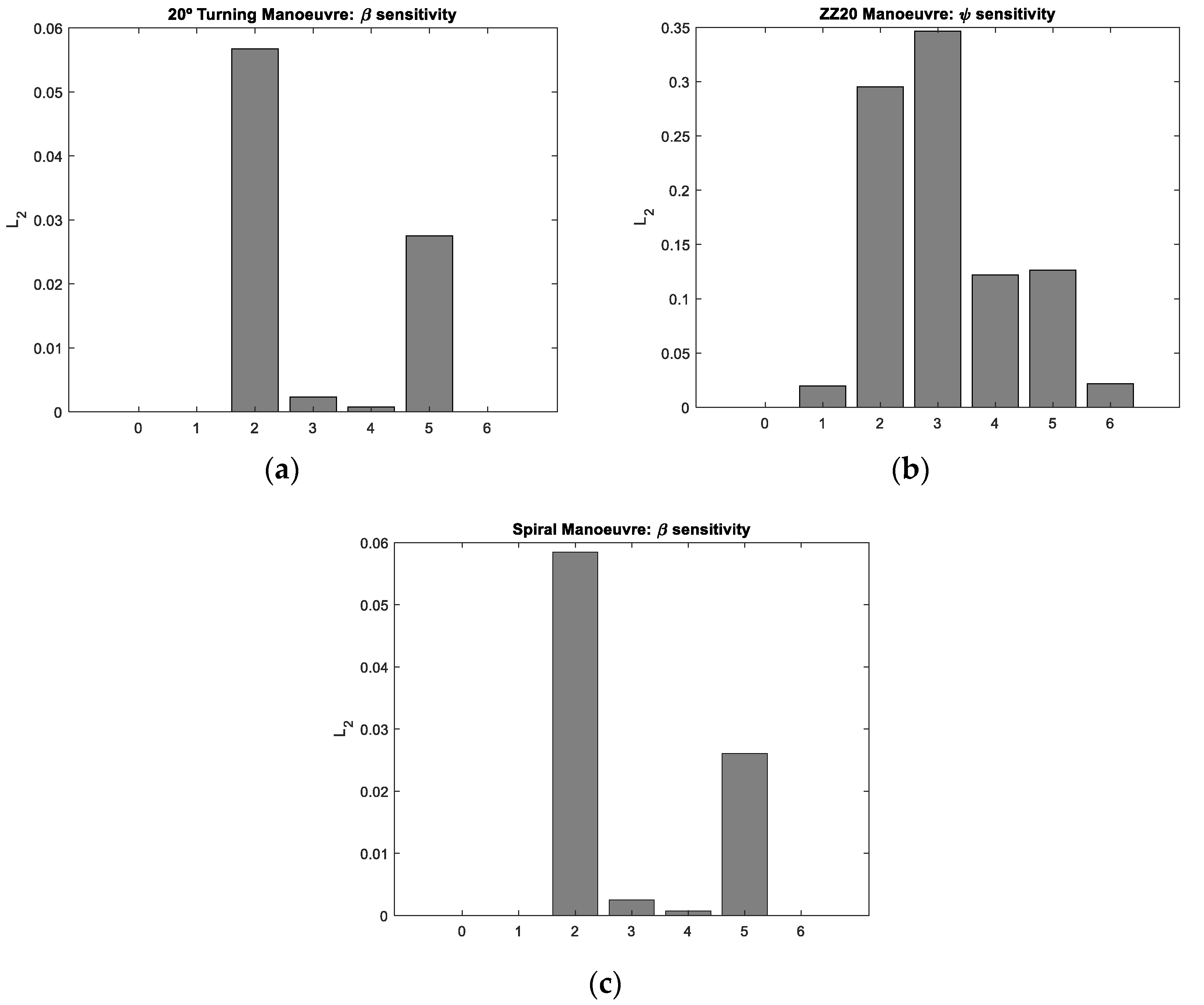
3.2. Sensitivity Analysis of the Manoeuvres for Perturbation of the Linear Coefficients

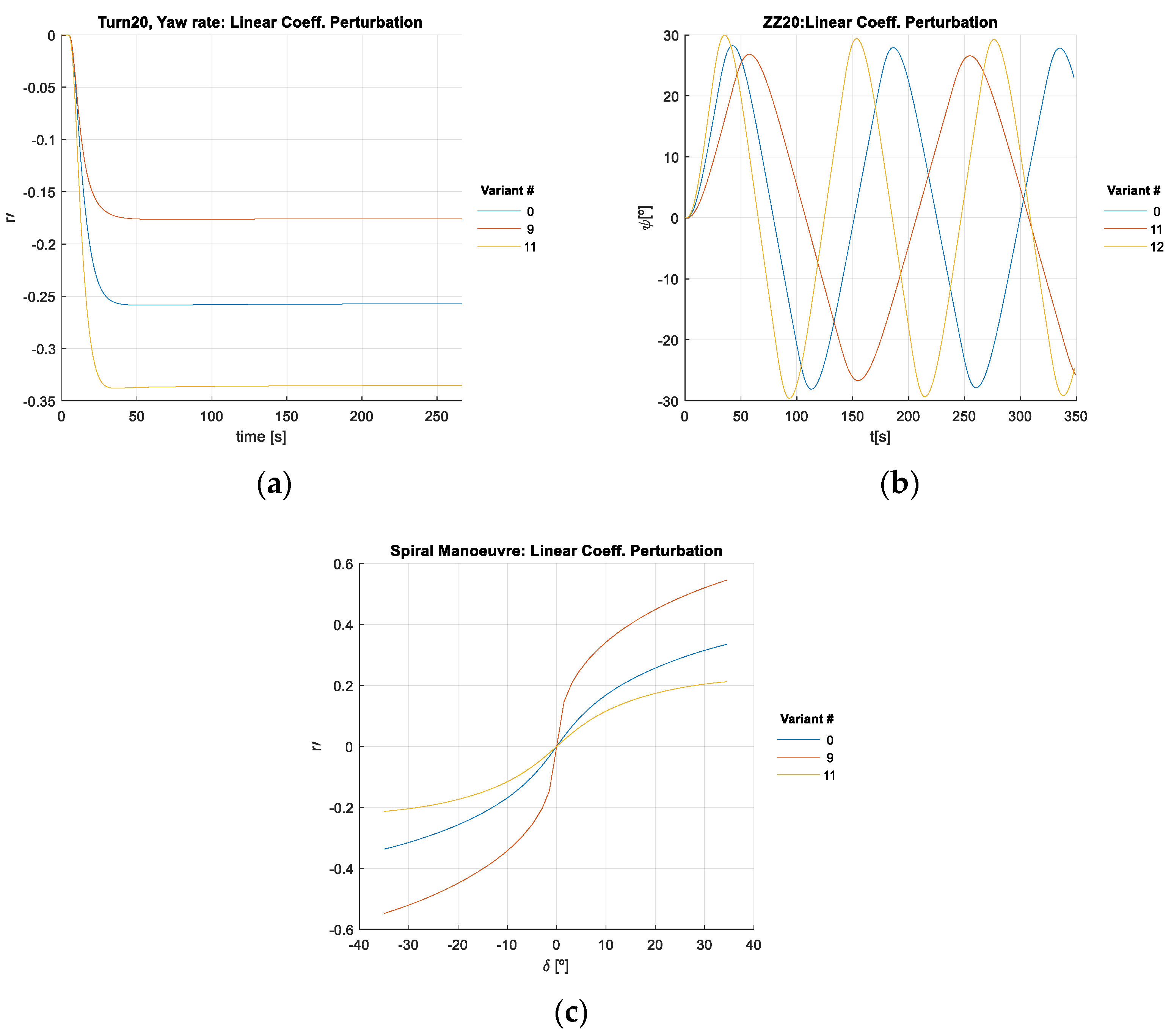
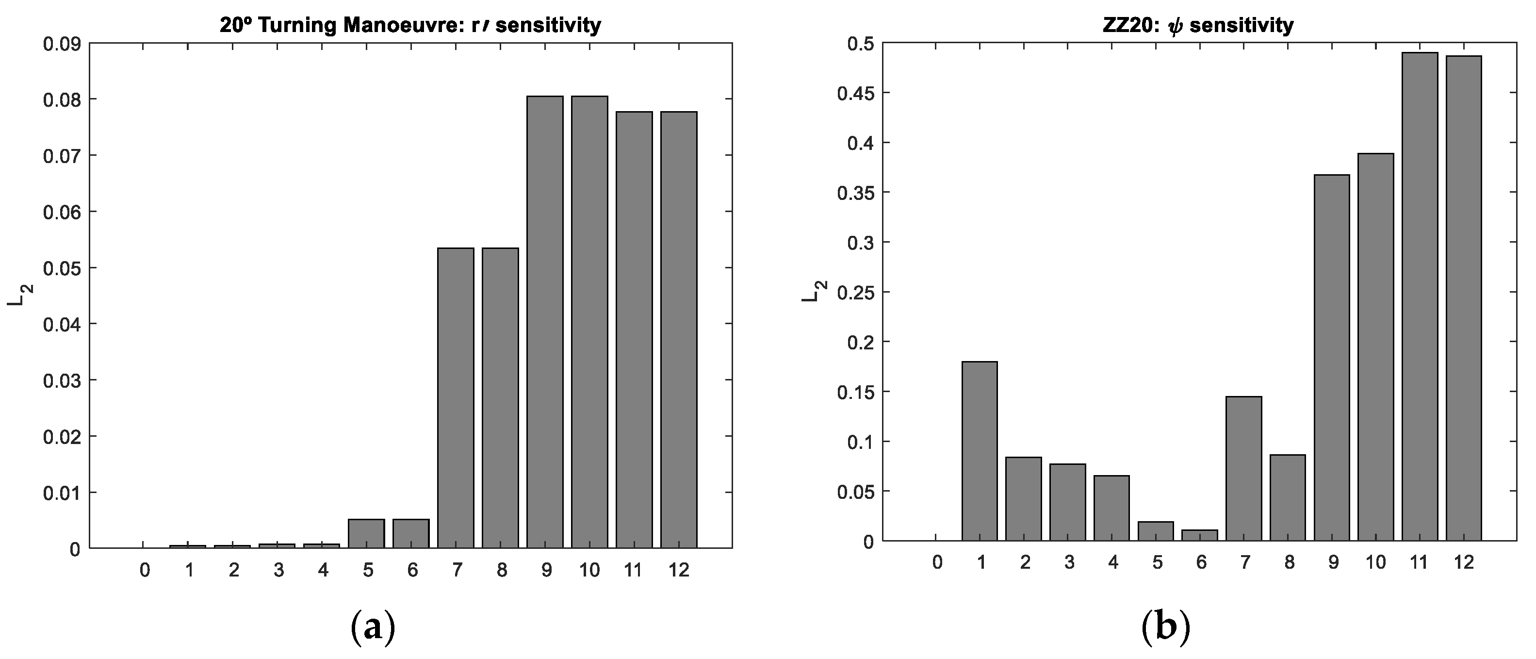
Figure 4 presents the reference run (variant #0) and the variants causing the maximum output parameter variation (maximum $L_2$) in some simulated manoeuvres when partial perturbation of the linear coefficients was performed.

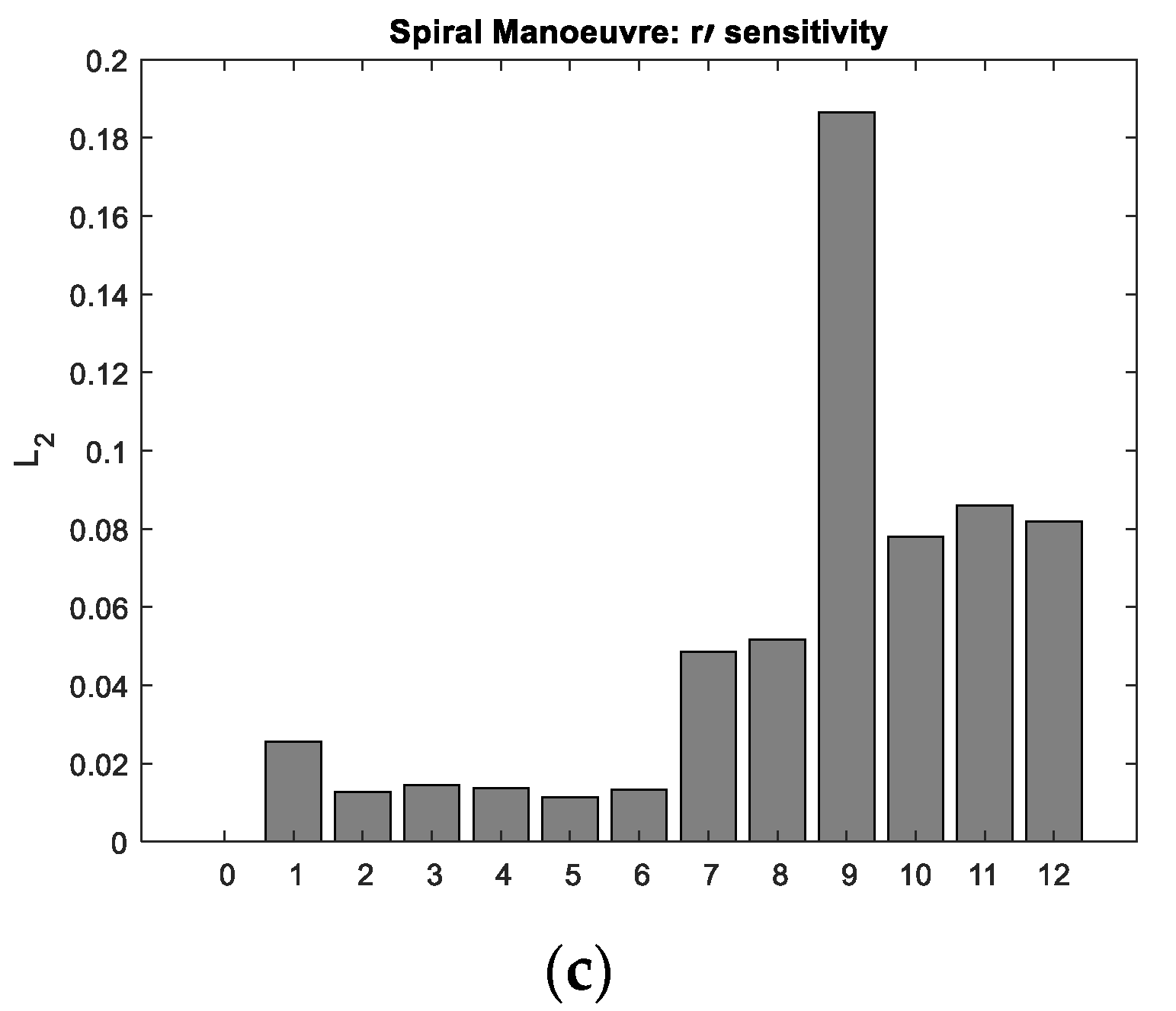
Figure 5 presents the $L_2$ values for the most influenced output parameters vs. variants in different manoeuvres.

Table 9. Most influential perturbation variants in all manoeuvres: linear coefficient perturbation.

Turning
Rudder order	Most influential variants
Output parameters	Yaw rate  $r\prime$	Drift angle  $\beta$	Velocity ratio  $V\prime$
$10°$	9, 10 11, 12 7, 8	3, 4 1, 2	9, 10 11, 12 7,8
$20°$	9, 10 11, 12	3, 4 1, 2	9, 10 11, 12
$30°$	11, 12 9, 10	3, 4 1, 2 5, 6	11, 12 9, 10
Zigzag
Rudder order	Most influential variants
Output parameters	Yaw rate  $r\prime$	Heading  $\psi$	Drift angle  $\beta$
$10°$	12, 11 10, 9 1,2	12, 11 10, 9 1,2	12, 11 10, 9 1,2
$20°$	12, 11 9, 10 1,2	11, 12 10, 9 1,2	11, 12 10, 9 1,2
Spiral
Rudder order	Most influential variants
Output parameters	Yaw rate  $r\prime$	Drift angle  $\beta$	Velocity ratio  $V\left(t\right)/V_0$
	9, 10 11, 12 7, 8	1, 2 3, 4 5, 6	9, 10 11 12 7, 8

presents the most influential perturbation variants in turning, zigzag and spiral manoeuvres for perturbation of the linear coefficients (LC), grouped as variants of similar sensitivity within 75–100% of the maximum $L_2$ value for each output variable.

Table 10. Synthesis of performance parameters’ $L_2$ results for the different manoeuvres: linear coefficient perturbation.

	$$\mathbf{Average} {\mathit{L}}_2$$
	Turn	Zigzag	Spiral
Yaw rate $r\prime$	$0.084$	$0.26$	$0.13$
Drift angle $\beta$	$0.022$	$0.081$	$0.026$
Velocity ratio $V\prime$	$0.024$	--	$0.044$
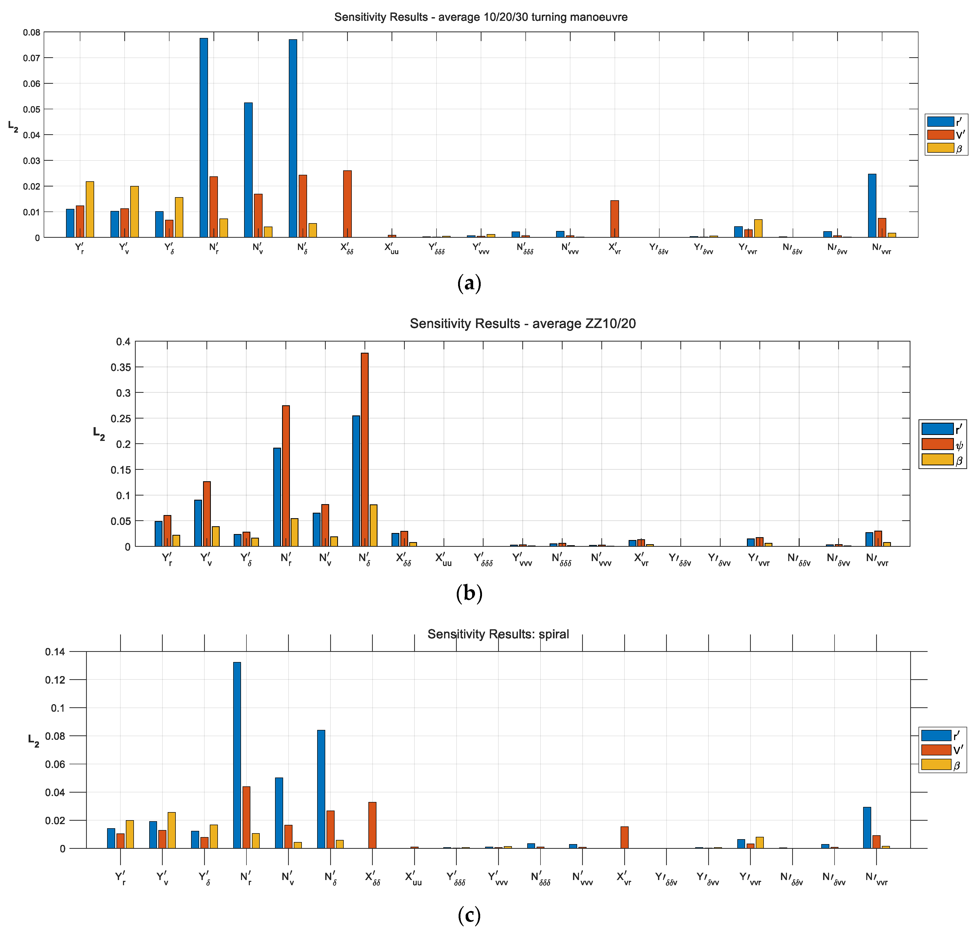
Heading $\psi$	--	$0.38$	--

presents a synthesis of $L_2$ results for the different performance parameters and the different manoeuvres. The values are an average of the maximum $L_2$ value of each kinematic variable, $y$, from the 10/20/30 turning manoeuvres—Equation (16)—and 10/20 Z-manoeuvres—Equation (17). For the spiral manoeuvre, as only one manoeuvre was performed, Table 10 presents the maximum $L_2$ value of the corresponding kinematic variable. Table 10,

Table 11. Most influential perturbation variants in all manoeuvres: NLS perturbation.

Turning
Rudder order	Most influential variants
Output parameters	Yaw rate  $r\prime$	Drift angle  $\beta$	Velocity ratio  $V\prime$
$10°$	9, 10	5, 6	3, 4
$20°$	9, 10 11, 12	5, 6	3, 4
$30°$	11, 12 9, 10	5, 6 7, 8	3, 4
Zigzag
Rudder order	Most influential variants
Output parameters	Yaw rate  $r\prime$	Heading  $\psi$	Drift angle  $\beta$
$10°$	3, 4	3, 4	3, 4
$20°$	3, 4	3, 4	3, 4
Spiral
Rudder order	Most influential variants
Output parameters	Yaw rate  $r\prime$	Drift angle  $\beta$	Velocity ratio  $V\left(t\right)/V_0$
	11, 12 9, 10	5, 6 7, 8	3, 4

,

Table 12. Synthesis of performance parameters’ $L_2$ results for the different manoeuvres: nonlinear single-variable coefficient (NLS) perturbation.

	$$\mathbf{Average} {\mathit{L}}_2$$
	Turn	Zigzag	Spiral
Yaw rate $r\prime$	$0.027$	$0.025$	$0.0034$
Drift angle $\beta$	$0.0013$	$0.0075$	$0.0013$
Velocity ratio $V\prime$	$0.027$	--	$0.0328$
Heading $\psi$	--	$0.029$	--

,

Table 13. Most influential perturbation variants in all manoeuvres: NLM perturbation.

Turning
Rudder order	Most influential variants
Output parameters	Yaw rate  $r\prime$	Drift angle  $\beta$	Velocity ratio  $V\prime$
$10°$	9, 10	3, 4 9, 10	2, 1 9, 10
$20°$	9, 10	3, 4 9, 10	2, 1 9, 10
$30°$	9, 10	3, 4	2, 1 9, 10
Zigzag
Rudder order	Most influential variants
Output parameters	Yaw rate  $r\prime$	Heading  $\psi$	Drift angle  $\beta$
$10°$	4, 3 9, 10 2, 1	4, 3 9, 10 2, 1	3, 4 9, 10 2, 1
$20°$	10, 9 3, 4 1, 2	10, 9 3, 4 1, 2	10, 9 3, 4 1, 2
Spiral
Rudder order	Most influential variants
Output parameters	Yaw rate  $r\prime$	Drift angle  $\beta$	Velocity ratio  $V\left(t\right)/V_0$
	9, 10	3, 4	2, 1 9, 10

and

Table 14. Synthesis of performance parameters’ $L_2$ results for the different manoeuvres: nonlinear multiple variable coefficient (NLM) perturbation.

	$$\mathbf{Average} {\mathit{L}}_2$$
	Turn	Zigzag	Spiral
Yaw rate $r\prime$	$0.028$	$0.059$	$0.029$
Drift angle $\beta$	$0.0078$	$0.02$	$0.008$
Velocity ratio $V\prime$	$0.0015$	--	$0.016$
Heading $\psi$	--	$0.069$	--

present the same information for nonlinear coefficients. This allows the highest-sensitivity performance parameters to be connected with the corresponding perturbation coefficient(s) for each manoeuvre.

$$L_{2y}^{avg}=\frac{L_2^{t10}+L_2^{t20}+L_2^{t30}}{n_t}$$

(16)

where $n_t$ is the number of turning manoeuvres,

$$L_{2y}^{avg}=\frac{L_2^{z10}+L_2^{z20}}{n_z}$$

(17)

From Table 10, it can be seen that the most sensitive output parameter was the yaw rate $r\prime$, followed by the velocity ratio $V\prime$, and the least sensitive was the drift angle $\beta$ in the average of the three turning manoeuvres. The output parameters $r\prime$ and $V\prime$ were most sensitive to perturbations of $N{\prime }_r$ and, with increasing rudder angles, $N{\prime }_{\delta }$. The output parameter $\beta$ was most sensitive to perturbations of $Y{\prime }_r$ and $Y{\prime }_v$; with increasing rudder angles, high sensitivity to $Y{\prime }_{\delta }$ also appeared.

The sensitivity results of the zigzag manoeuvre showed that the output parameters $\psi , r\prime$ and $\beta$ had the highest sensitivity to perturbation in $N{\prime }_{\delta }$, closely followed by $N{\prime }_r$. The highest sensitivities were those of the output parameters $\psi$ and $r\prime$. The drift angle $\beta$ was the least sensitive output parameter, with about 23% of the sensitivity of $\psi$.

The output parameter most sensitive to the spiral manoeuvre was the yaw rate, $r\prime$. This variable was most sensitive to $N{\prime }_r$, but $N{\prime }_{\delta }$ also exerted a significant degree of influence. $V\prime$ was sensitive to the same coefficients as $r\prime$ but had much less sensitivity (about 34% of the sensitivity of $r\prime$). $\beta$ was the least sensitive output variable (about 17% of the sensitivity of $r\prime$).

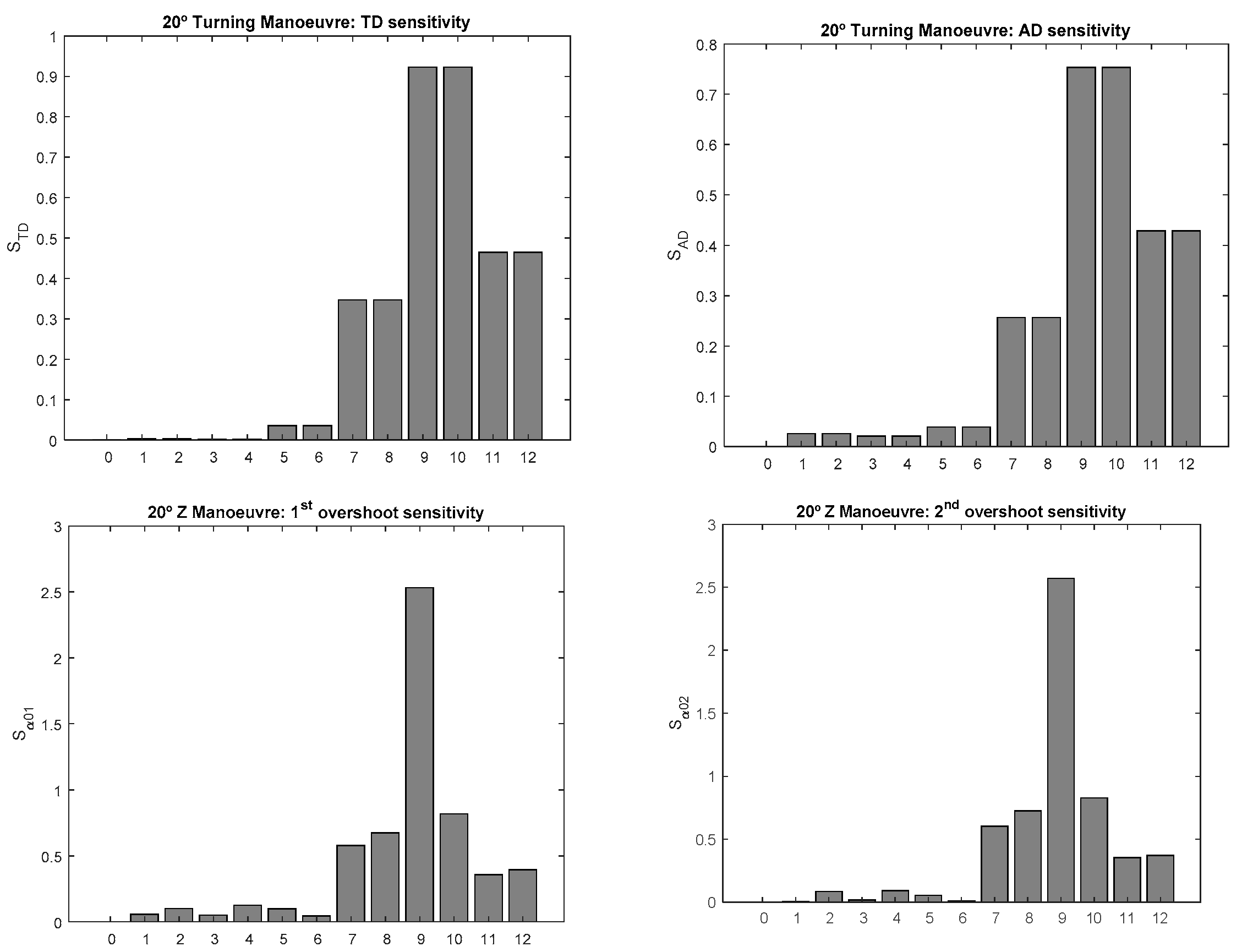
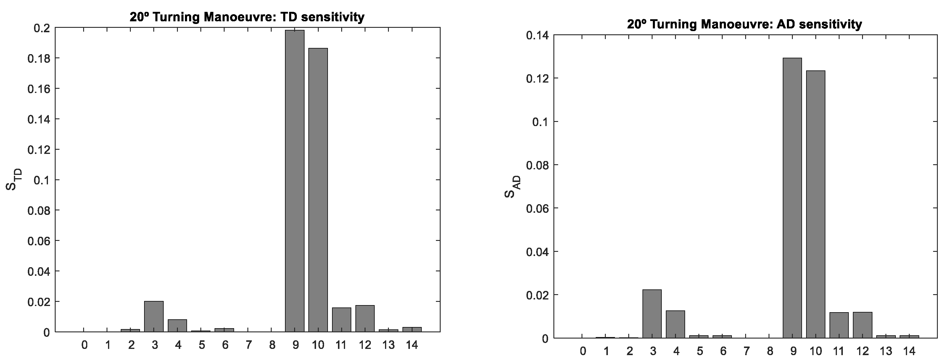
In papers dedicated to this subject, the authors make use of two performance parameter types: the kinematic variables used here, or the classical IMO manoeuvring performance criteria variables. To show how the sensitivity of each group of the performance parameters behaves, a comparison study was made here of these sensitivity results with those calculated using classic performance criteria, such as the tactical diameter (TD), advance (AD) and peak overshoots (${\alpha }_{01}$, ${\alpha }_{02}$) as prescribed by the IMO Standards for Ship Manoeuvrability [32] and reported by Ishiguro et al. [21]. As in [21], the sensitivity index $S_k$ represents the ratio of change in the estimated results when each parameter is changed by 50%. It becomes 1.0 when the estimated relevant index increases 50% upon the 50% increase of a given parameter. Absolute values of variation were chosen, and graphical results are presented in Figure 6.

The results show that for the turning manoeuvre, the most influential coefficients were the same as those obtained using the kinematic variables $r\prime$ and $V\prime$: $N{\prime }_r$, $N{\prime }_{\delta }$ and $N{\prime }_v$. These results are in line with those obtained by Ishiguro et al. [21] for $N{\prime }_r$ and $N{\prime }_{\beta }$, since $N{\prime }_{\delta }$ was not part of their model. $N{\prime }_r$ also appears as one of the most influential LCs (closely after $N{\prime }_{\beta }$) in the work by Kose and Misiag [19,20] that used the peak overshoots, tactical diameter, advance and transfer as performance variables.

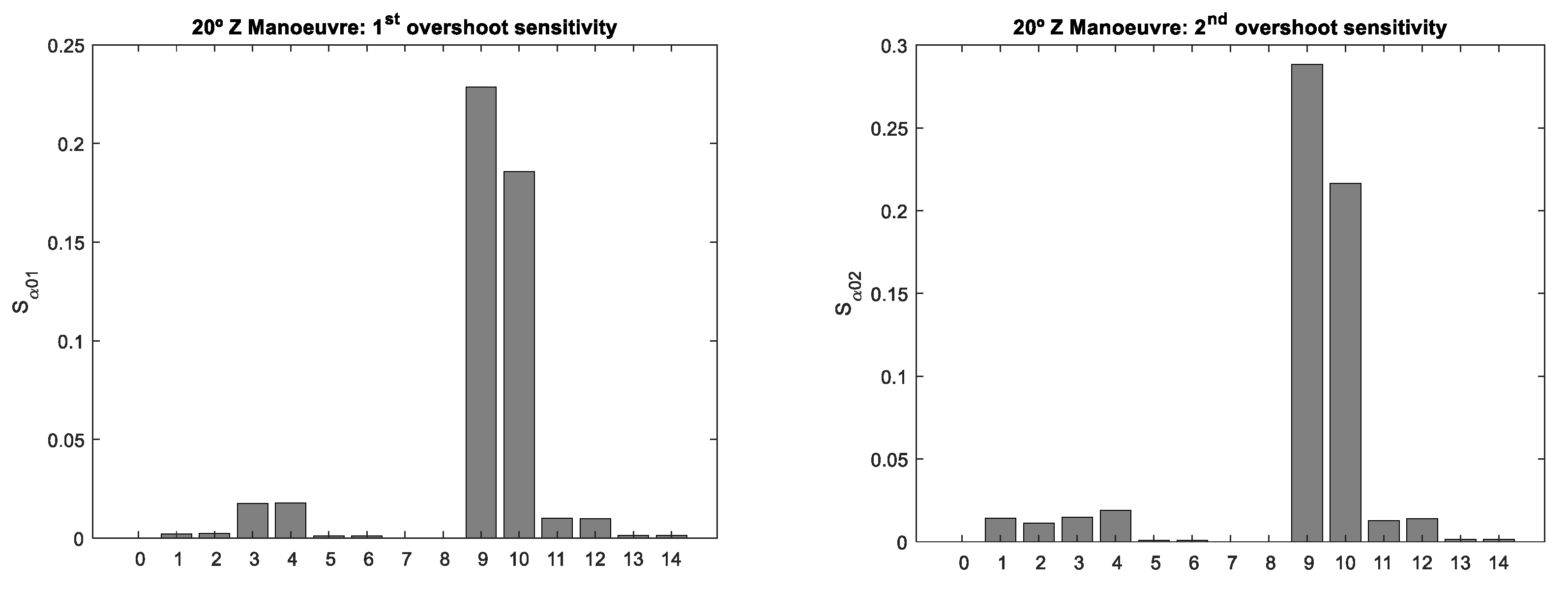
For the zigzag manoeuvre, both overshoots were most sensitive to $N{\prime }_r$. Sensitivity to $N{\prime }_v$ and $N{\prime }_{\delta }$ also existed, but was less evident than when using the kinematic variables. Sensitivity to $Y{\prime }_v$ did not appear to show any relevance. Interestingly the sensitivity results when using kinematic variables were closer to those reported by Ishiguro et al. [21], while the sensitivity results from the use of overshoots differed from those in [21] in terms of sensitivity to $Y{\prime }_v$.

$N{\prime }_v$ and $Y{\prime }_v$ do not appear as clearly as the most influential linear coefficients in the referenced works. It is believed this is because this research was conducted on a naval combatant hull mathematical model, with a different underwater hull shape. As shown, the sensitivity analysis using some of the same performance parameters as were used by Ishiguro et al. [21] and Kose and Misiag [19,20] confirmed the results of the sensitivity analysis performed in this work, which used the kinematic variables as the performance parameters. In addition, in the present model, the linear coefficient $N{\prime }_{\delta }$ was shown to be influential, although it was not part of the MMG models used by the referenced authors.

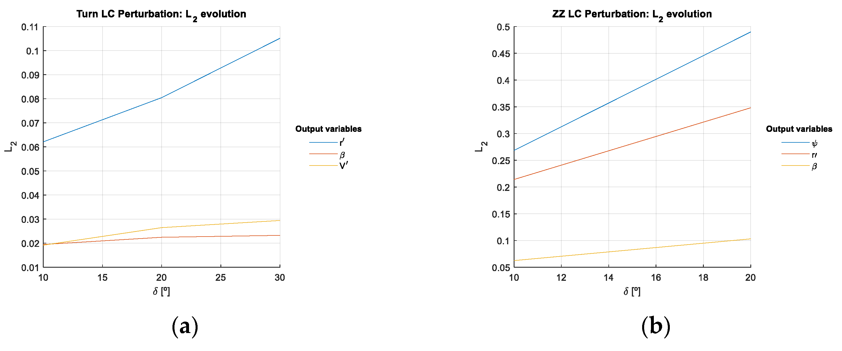
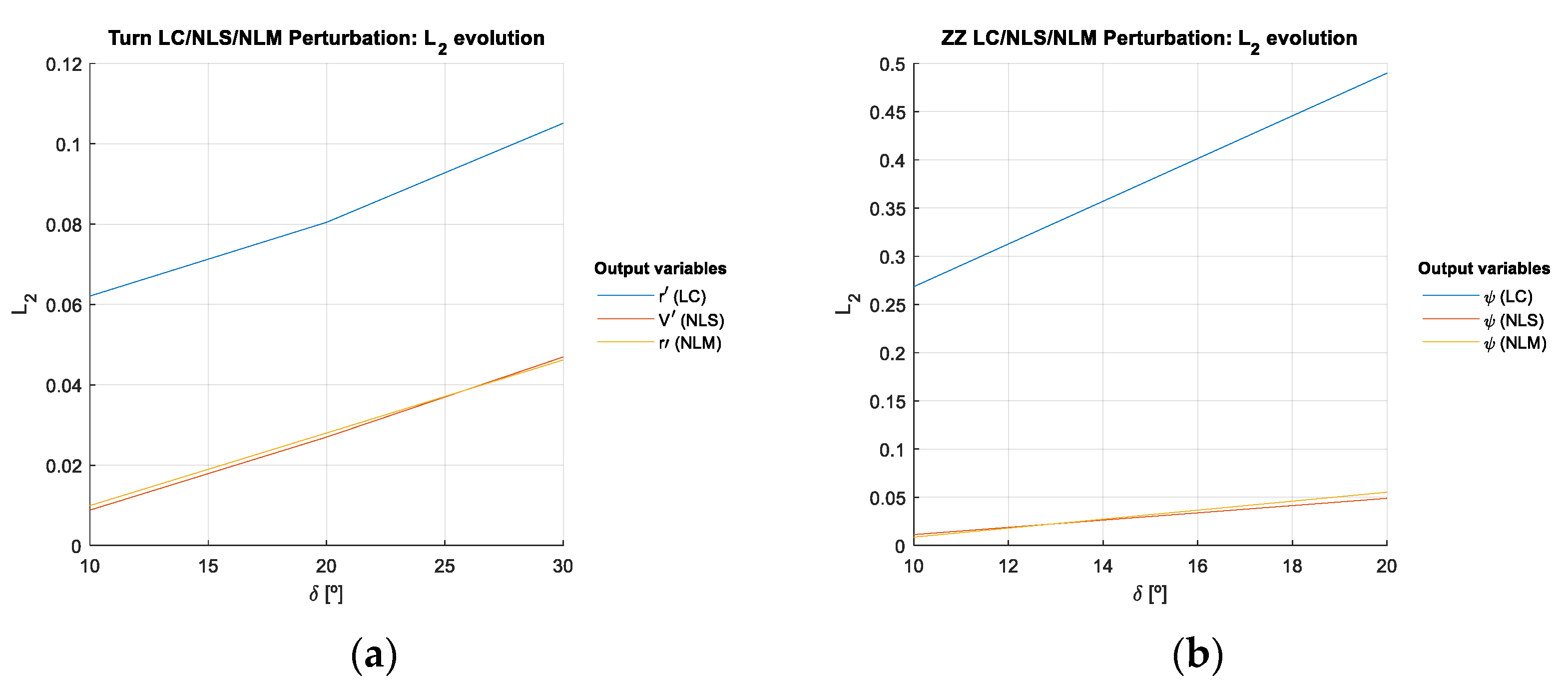
The sensitivity increased with increasing rudder angle but with different behaviours from each output parameter, as can be observed in Figure 7. This effect was indirectly visible in previous works regarding Z-manoeuvres, but not in works regarding the turning manoeuvre, because usually only one 35° turning manoeuvre is studied, e.g., Kose and Misiag, [19], Ishiguro et al., [21] and Rhee and Kim [22].

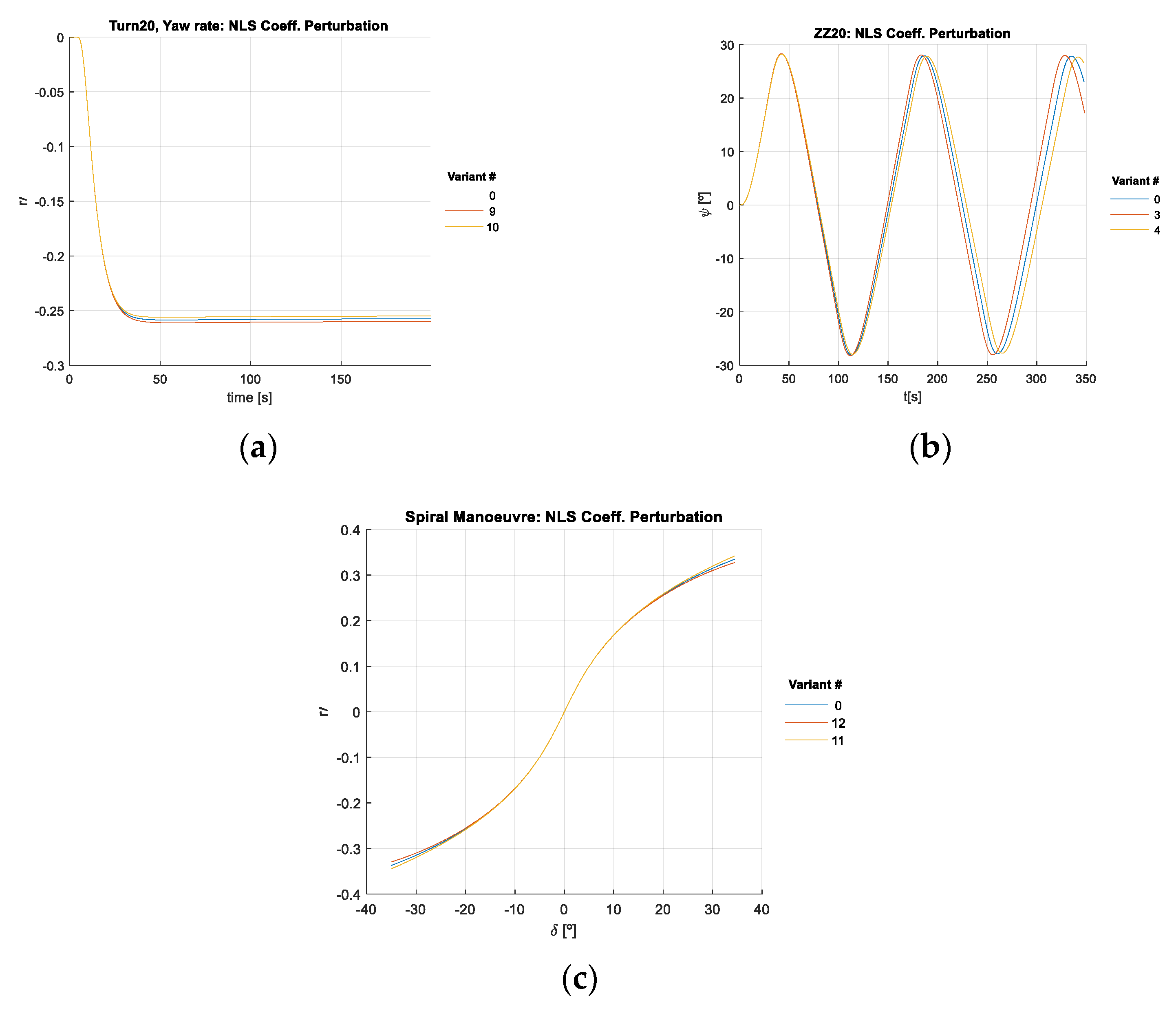
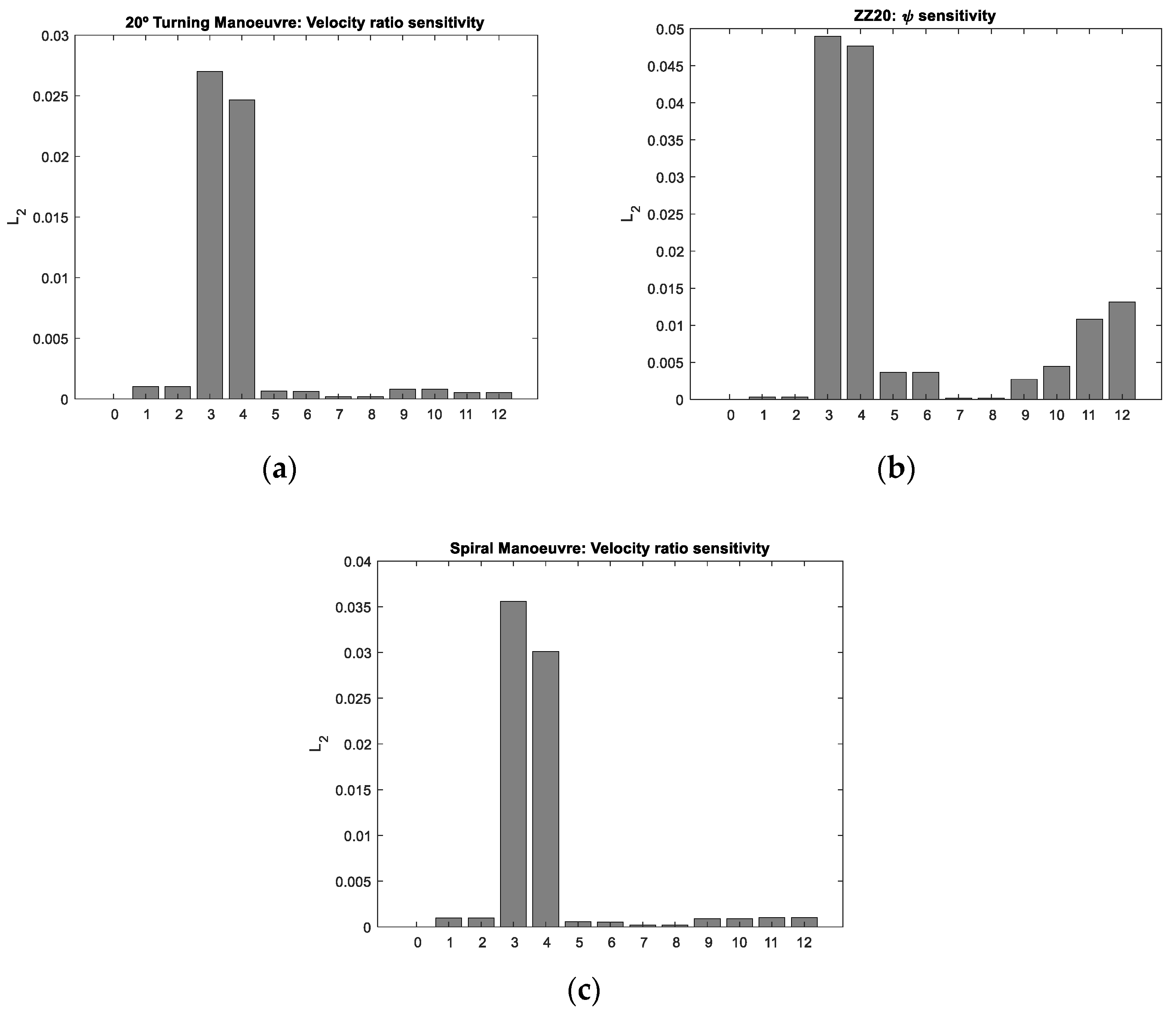
3.3. Sensitivity Analysis of the Manoeuvres for Perturbation of the Nonlinear Single-Variable Coefficients

Figure 8 presents the reference run (variant #0) and the variants causing the maximum output parameter variation in some of the simulated manoeuvres when a partial perturbation of the nonlinear single variable coefficients was performed.

Figure 9 presents the $L_2$-metric graphs of the sensitivity analysis for the most influenced output parameters vs. variant for NLS perturbation.

Table 11 presents the most relevant perturbation variants in the studied manoeuvres for NLS perturbation.

Table 12 presents a synthesis of performance parameters’ $L_2$ results for the different manoeuvres resulting from NLS perturbation.

Depending on the manoeuvre, the output parameters most sensitive to NLS perturbation were: the velocity ratio, $V\prime$ (turning and spiral), and $\psi \mathrm{and} r\prime$ (zigzag), which were essentially sensitive to $X{\prime }_{\delta \delta }$. Comparing the levels of sensitivity of nonlinear single-variable coefficients with those of linear coefficients, the first was on average about 2% of the latter. Therefore, the mathematical model was less sensitive to the nonlinear single-variable parameters, which in this model were of the second and third order, the latter with a diffuse physical meaning, while the former was the hull and rudder nonlinear drag: $X{\prime }_{uu} \mathrm{and} X{\prime }_{\delta \delta },$ respectively.

The most sensitive output parameter observed for the perturbation of the nonlinear single-variable coefficients (NLSs) was $V\prime$ in spiral and turning manoeuvres and $\psi$ and $r\prime$ in Z manoeuvres. The most relevant NLS coefficient, $X{\prime }_{\delta \delta }$, was the rudder nonlinear drag for all manoeuvres.

Wang et al. [24] present a sensitivity analysis using the direct method and Wang et al. [18] present a sensitivity analysis using the indirect method, both using the same 4DOF mathematical model of a container ship, with 18 hydrodynamic coefficients in the surge equation and 28 in each of the sway equation and yaw equation. Bearing in mind the different hull types in this study and those referenced, and also the different metrics, it is interesting to note that the results obtained by Wang et al. [18] for the surge motion using the indirect method also showed a high sensitivity of the model to $X{\prime }_{\delta \delta }$. $X{\prime }_{uu}$ appeared as the fourth most influential coefficient in surge motion, while in the present paper it was almost negligible.

The results were very different when using the direct method, wherein $X{\prime }_{uu}$ was the third most influential coefficient and $X{\prime }_{\delta \delta }$ was almost negligible. These results may indicate that further studies could be done on the nature and adequacy of the direct method vs. the indirect method, and the indirect method may work well and be more informative if using kinematic variables as output parameters instead of IMO criteria/classical output parameters of the turning and Z-manoeuvres.

From what has been discussed so far, it is clear that the sensitivity analysis using kinematic variables and various rudder orders (in turning and Z manoeuvres) introduces complexity to the analysis, but shows some kinematic variables at a consistently higher level of sensitivity, as was the case for $r\prime$ in all manoeuvres and heading $\psi$ in Z-manoeuvres, and shows that the influence of the model coefficients, or, in other words, the sensitivity to the kinematic variables, evolves with the rudder angle.

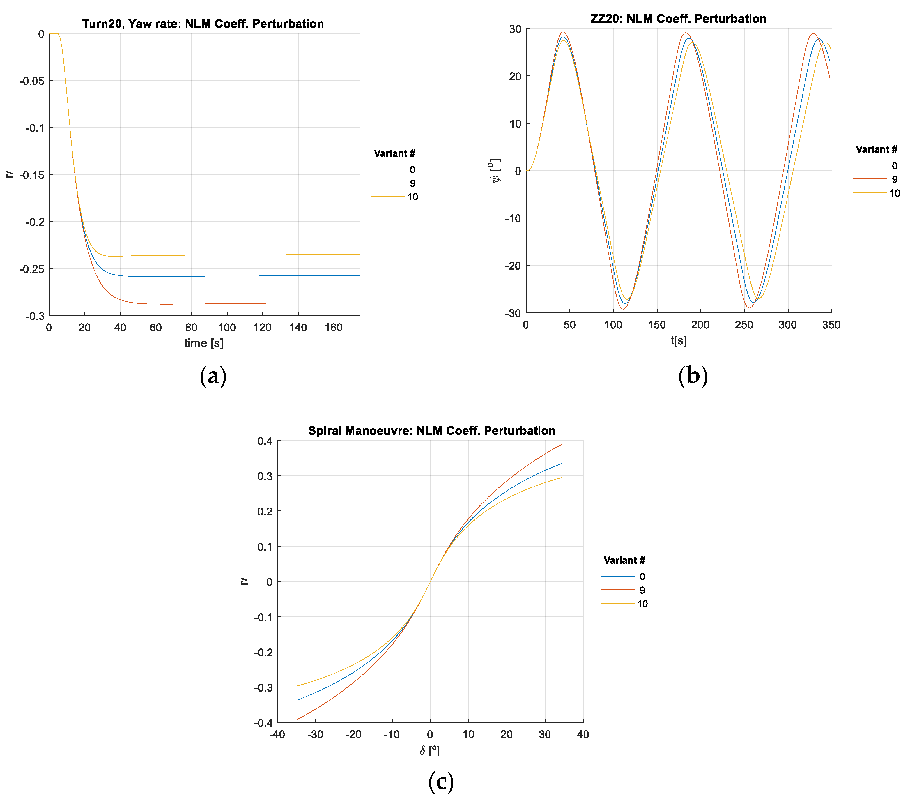
3.4. Sensitivity Analysis of the Manoeuvres for Perturbation of the Nonlinear Multivariable Coefficients

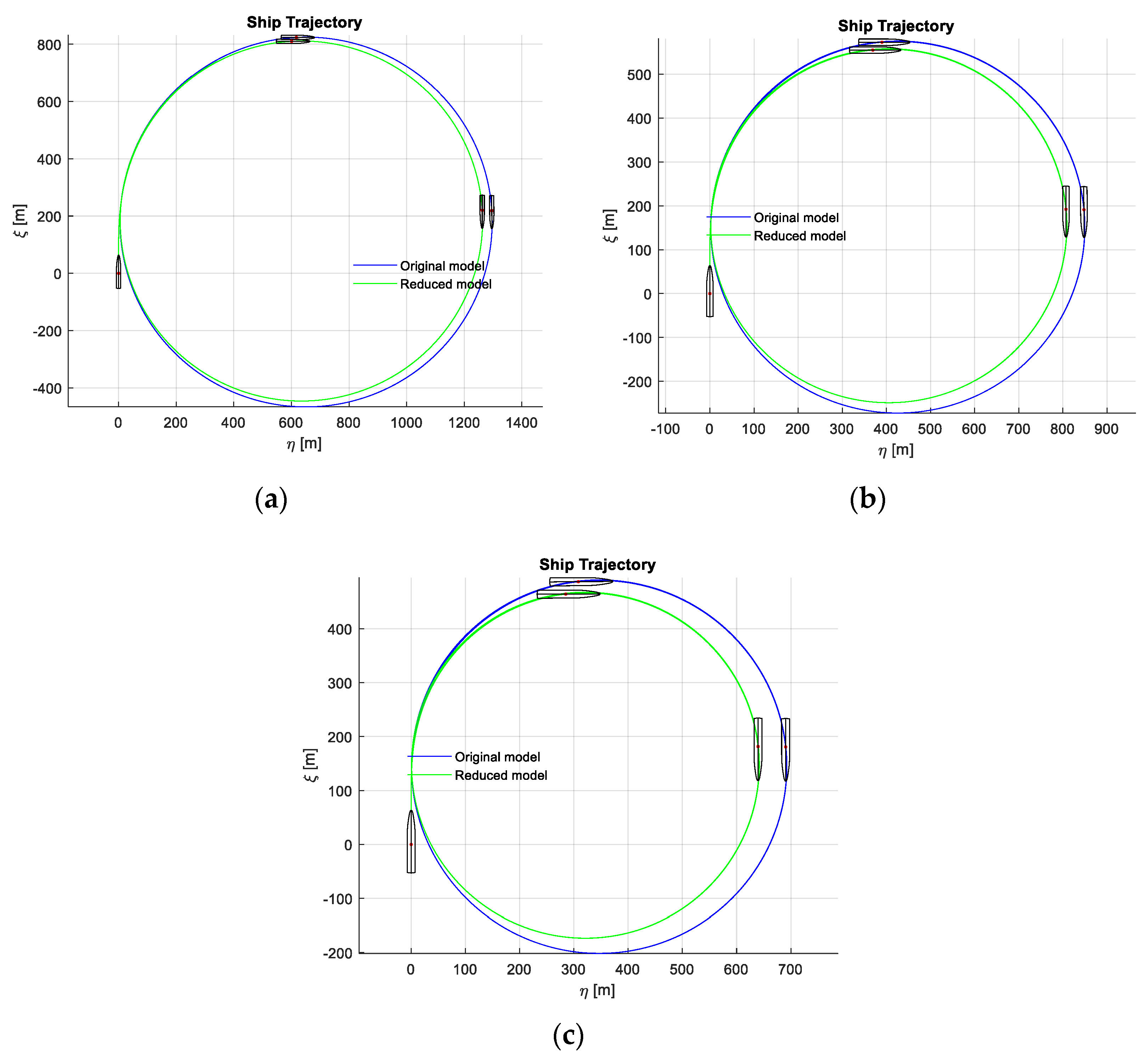
Figure 10 presents the reference run (variant #0) and the bounds of the ship behaviour in some of the simulated manoeuvres when partial perturbation of the nonlinear multivariable coefficients was performed.

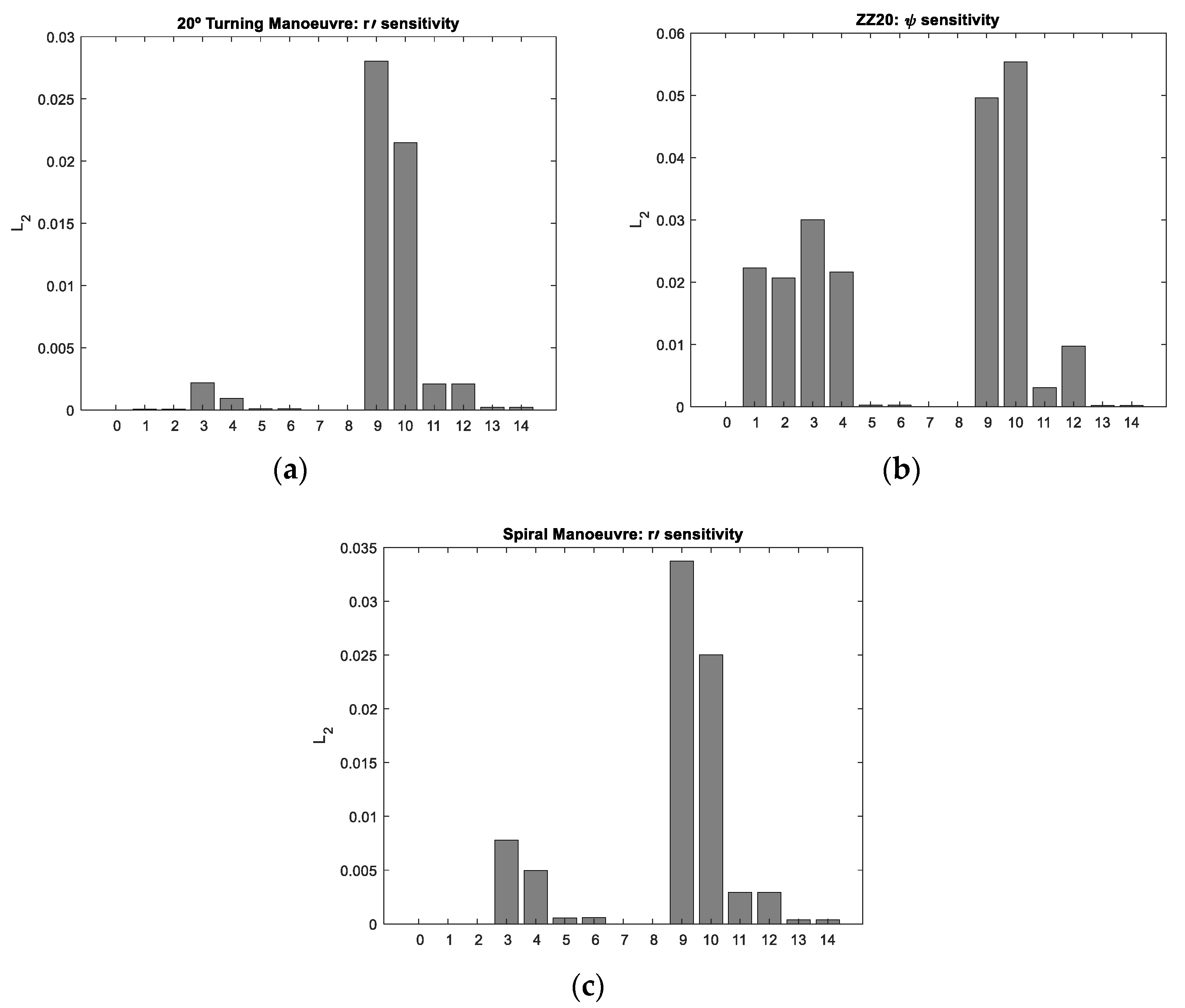
Table 13 presents the most relevant perturbation variants in the studied manoeuvres for NLS perturbation.

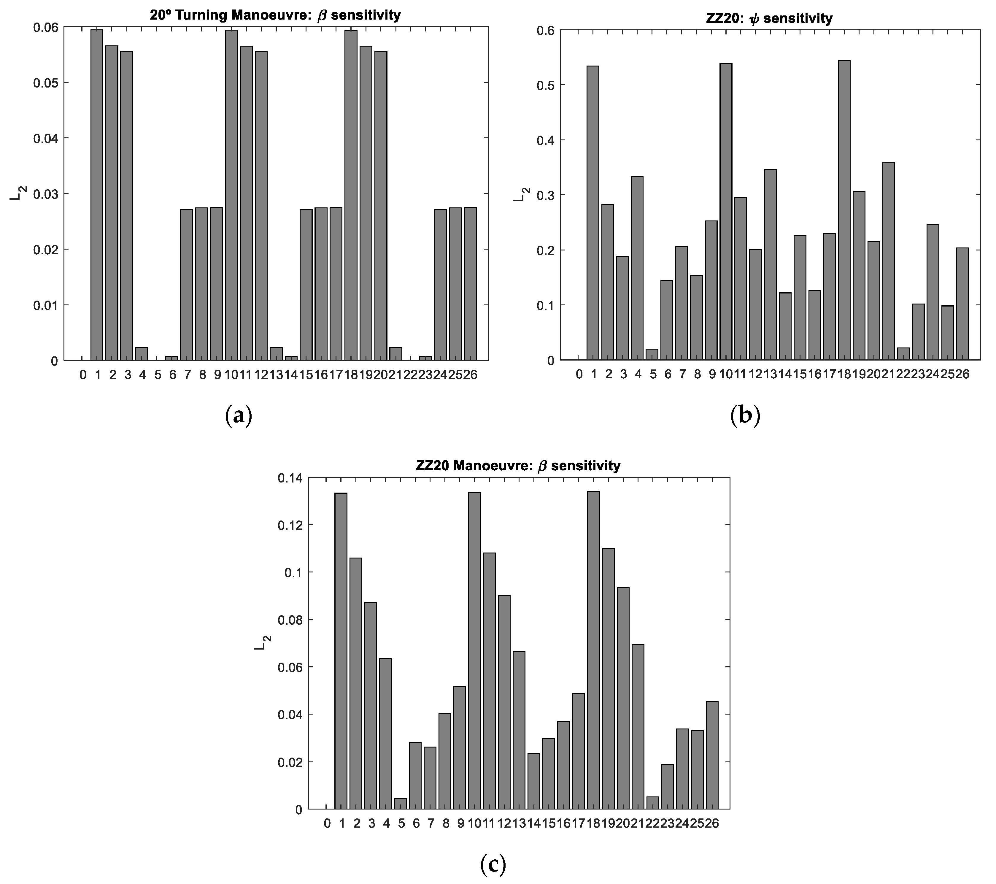
Figure 11 presents the $L_2$-metric graphs of the sensitivity analyses for the most influenced output parameters vs. variants for NLM perturbation.

Table 14 presents a synthesis of performance parameters’ $L_2$ results for the different manoeuvres resulting from NLM perturbation.

For the turning manoeuvre, the levels of sensitivity of the NLM coefficients were on average about 24% of those arising from linear coefficients (LC). Above this level of sensitivity were the coefficients $X{\prime }_{vr}$,$N{\prime }_{vvr}$ and $Y{\prime }_{vvr}$. Comparing the levels of sensitivity of these NLM coefficients to those of nonlinear single-variable coefficients (NLS), they were on average about 500% of the latter.

In the zigzag manoeuvre, the sensitivity of all output parameters was the highest for $N{\prime }_{vvr}$ and ${Y^{\prime }}_{vvr}$. For Z10, the sensitivity was highest for ${Y^{\prime }}_{vvr}$ and for Z20, the sensitivity was highest for ${N^{\prime }}_{vvr}$. The output parameters also showed non-negligible sensitivity to $X{\prime }_{vr}$, although the relative influence diminished as the rudder angle increased. Comparing these levels of sensitivity to those relative to linear coefficients, they were on average about 11% of the latter. Above this level of sensitivity were the coefficients $N{\prime }_{vvr}$ and $Y{\prime }_{vvr}$. Comparing the levels of sensitivity of these coefficients to those of NLS coefficients, they were on average about 200% of the latter.

As in the other manoeuvres, in the spiral manoeuvre, the sensitivity to the NLM coefficients was more significant than that observed for the NLS coefficients and less significant than that observed for the linear coefficients.

Therefore, on average, the mathematical model was much more sensitive to the NLM coefficients than to the NLS coefficients for all manoeuvres.

Figure 12 presents the sensitivity of the model using IMO manoeuvring performance variables as explained in Subsection 3.2.

Using the classical output parameters (Figure 12), it is clear that for both the turning manoeuvre and the Z-manoeuvre, there was one influential coefficient, $N{\prime }_{vvr}$, which is in line with the results obtained using the kinematic variables, but somewhat less informative, since all the remaining coefficients were residual while the sensitivity results using kinematic variables evinced other relevant NLM coefficient sensitivity indices, as shown in Figure 11 and Table 13. It is also apparent that there is an agreement between the two methods in terms the highest sensitivity of the model being to linear coefficients by different orders of magnitude relative to nonlinear multivariable coefficients.

All in all, the most sensitive output parameter was the yaw rate $r\prime$ for turning and spiral manoeuvres, and $\psi$ (closely followed by $r\prime$) for the zigzag manoeuvre. The most influential NLM coefficients in terms of the high sensitivities of these kinematic parameters were ${N^{\prime }}_{vvr}$ and ${Y^{\prime }}_{vvr}$, and ${X^{\prime }}_{vr}$ was shown to be relevant in influencing $V\prime$. These results are not directly comparable to those obtained by Ishiguro et al. [21] since different model coefficients were used. However, one of the two NLM coefficients with the highest sensitivity reported in [21] was $N{\prime }_{\beta \beta r}$, an analogue to $N{\prime }_{vvr}$, which is also the only one of these NLMs shown to be relevant by Wang et al. [18,24]. The fact that ${Y^{\prime }}_{vvr}$ and ${X^{\prime }}_{vr}$ do not appear in the reduced model with the highest sensitivity values in the Wang et al. papers [18,24], although they were part of the initial group of coefficients under analysis, may be related to the different hull shapes under consideration.

Regarding the sensitivity analysis vs. rudder angle, in general, the sensitivity increased with increasing rudder angle, as seen in Figure 7 and addressed from a different perspective in Figure 13, which compares the relative values of sensitivity of the performance kinematic parameters with the highest sensitivity index values in the turning and Z-manoeuvres for LC ($N_r, N_{\delta })$, NLS ($X_{\delta \delta }$), and NLM ($N_{vvr}$) perturbations.

4. Discussion

4.1. Sensitivity Study and Analysis

From the perspective of the relevance and adequacy of the chosen kinematic variables as performance parameters for the turning manoeuvre, the most relevant performance parameters were the yaw rate $r\prime$ and velocity ratio $V\prime$. The same relevance in opposite order was observed for the spiral manoeuvre. For the Z-manoeuvre, the highest sensitivity was observed for $\psi$ and $r\prime$. However, the three kinematic variables $\psi ,r\prime \mathrm{and} \beta$ seem to be relevant output parameters in the sensitivity analysis of the zigzag manoeuvre, and globally this manoeuvre generated the highest values of the $L_2$ sensitivity index (see Figure 7b and Figure 13b, Table 10 and Table 14).

The effects on drift angle $\beta \prime$ were globally lower for all manoeuvres but not negligible (see

Table 15. Most influential coefficients in turning manoeuvre by kinematic variable.

	Coefficient Type
	Linear			Nonlinear Multivariable		Nonlinear Single Variable
$\mathit{r}\prime$	$N{\prime }_r$	$N{\prime }_{\delta }$	$N{\prime }_v$	$N{\prime }_{vvr}$	$Y{\prime }_{vvr}$	$N{\prime }_{vvv}$	$N{\prime }_{\delta \delta \delta }$
$L_2^{avg}$	$0.08$	$0.077$	$0.053$	$0.025$	$0.0043$	$0.0024$	$0.0022$
$L_2^{ratio}$, percent	$100$	$97$	$67$	$31$	$5$	$3$	$3$
$\mathit{V}\prime$	$N{\prime }_r$	$N{\prime }_{\delta }$	$N{\prime }_v$	${\mathrm{X}\prime }_{vr}$	$N{\prime }_{vvr}$	${\mathrm{X}\prime }_{\delta \delta }$
$L_2^{avg}$	$0.023$	$0.023$	$0.016$	$0.014$	$0.0075$	$0.026$
$L_2^{ratio}$, percent	$29$	$29$	$21$	$18$	$9$	$33$
$\mathit{\beta }$	$Y{\prime }_r$	$Y{\prime }_v$	$Y{\prime }_{\delta }$	$Y{\prime }_{vvr}$	$N{\prime }_{vvr}$	$Y{\prime }_{vvv}$	$Y{\prime }_{\delta \delta \delta }$
$L_2^{avg}$	$0.022$	$0.020$	$0.015$	$0.0069$	$0.0017$	$0.0012$	$0.0004$
$L_2^{ratio}$, percent	$27$	$25$	$19$	$9$	$2$	$2$	$1$

,

Table 16. Most influential coefficients in zigzag manoeuvre by kinematic variable.

	Coefficient Type
	Linear			Nonlinear Multivariable		Nonlinear Single Variable
$\mathit{\psi }$	$N{\prime }_{\delta }$	$N{\prime }_r$	${\mathrm{Y}\prime }_v$	$N{\prime }_{vvr}$	$Y{\prime }_{vvr}$	${\mathrm{X}\prime }_{\delta \delta }$	${\mathrm{Y}\prime }_{vvv}$
$L_2^{avg}$	$0.38$	$0.27$	$0.13$	$0.03$	$0.017$	$0.029$	$0.0027$
$L_2^{ratio}$	$100$	$73$	$34$	$8$	$5$	$8$	$1$
$\mathit{r}\prime$	$N{\prime }_{\delta }$	$N{\prime }_r$	${\mathrm{Y}\prime }_v$	$N{\prime }_{vvr}$	$Y{\prime }_{vvr}$	$X{\prime }_{\delta \delta }$	$Y{\prime }_{vvv}$
$L_2^{avg}$	$0.25$	$0.19$	$0.09$	$0.027$	$0.015$	$0.025$	$0.0023$
$L_2^{ratio}$	$66$	$50$	$24$	$7$	$4$	$7$	$1$
$\mathit{\beta }$	$N{\prime }_{\delta }$	$N{\prime }_r$	${\mathrm{Y}\prime }_v$	$N{\prime }_{vvr}$	$Y{\prime }_{vvr}$	$X{\prime }_{\delta \delta }$	$Y{\prime }_{vvv}$
$L_2$ value	$0.081$	$0.054$	$0.038$	$0.0077$	$0.0058$	$0.0068$	$0.00079$
$L_2^{ratio}$	$22$	$14$	$10$	$2$	$2$	$2$	$0.2$

and

Table 17. Most influential coefficients in spiral manoeuvre by kinematic variable.

	Coefficient Type
	Linear			Nonlinear Multivariable			Nonlinear Single Variable
$\mathit{r}\prime$	$N{\prime }_r$	$N{\prime }_{\delta }$	${\mathrm{N}\prime }_v$	$N{\prime }_{vvr}$	$Y{\prime }_{vvr}$	$N{\prime }_{\delta vv}$	${\mathrm{N}\prime }_{\delta \delta \delta }$	${\mathrm{N}\prime }_{vvv}$
$L_2^{avg}$	$0.13$	$0.085$	$0.051$	$0.029$	$0.0064$	$0.0029$	$0.0034$	$0.0029$
$L_2^{ratio}$	$100$	$64$	$38$	$22$	$5$	$2$	$3$	$2$
$\mathit{V}\prime$	$N{\prime }_r$	$N{\prime }_{\delta }$	${\mathrm{N}\prime }_v$	${\mathrm{X}\prime }_{vr}$	${\mathrm{N}\prime }_{vvr}$	$Y{\prime }_{vvr}$	${\mathrm{X}\prime }_{\delta \delta }$
$L_2^{avg}$	$0.044$	$0.027$	$0.017$	$0.016$	$0.0092$	$0.0032$	$0.033$
$L_2^{ratio}$	$33$	$20$	$13$	$12$	$7$	$2$	$25$
$\mathit{\beta }$	${\mathrm{Y}\prime }_v$	${\mathrm{Y}\prime }_r$	${\mathrm{Y}\prime }_{\delta }$	$Y{\prime }_{vvr}$	$N{\prime }_{vvr}$	$Y{\prime }_{\delta vv}$	$Y{\prime }_{vvv}$	$Y{\prime }_{\delta \delta \delta }$
$L_2^{avg}$	$0.026$	$0.02$	$0.017$	$0.0083$	$0.0017$	$0.0007$	$0.0014$	$0.0007$
$L_2^{ratio}$	$19$	$15$	$13$	$6$	$1$	$0.5$	$1$	$0.5$

). Therefore, all these kinematic variables seem adequate for the present sensitivity analysis. However, in terms of efficiency of the sensitivity analysis (fewer manoeuvres for the same level of accuracy), it seems that the spiral manoeuvre, using as performance parameters the kinematic variables $r\prime , \beta$ and $V^{\prime }$, may be enough for an adequate sensitivity analysis. This is a new approach relative to the choice of performance parameters and manoeuvre type used for sensitivity analysis, and appears to be valid at least for typical naval combatants of the corvette or frigate hull types.

The average $L_2$ sensitivity index is given by

$$L_2^{ratio}=\frac{L_2^{avg}}{L_2^{max}}$$

(18)

Observing the sensitivity from the perspective of the output parameters’ sensitivity to all (LC, NLS and NLM) coefficients, Table 15 presents the average $L_2$ sensitivity indices (Equation (16)) from the 10/20/30 turning manoeuvres for each partial perturbation, and the relative sensitivity ($L_2$ ratio) to the most influential coefficient.

The most influential coefficients were the linear ones, followed by the nonlinear multivariable coefficients and the least influential were the nonlinear single-variable coefficients. The NLS coefficients were almost irrelevant, except for the coefficient ${\mathrm{X}\prime }_{\delta \delta }$ for the output variable velocity ratio $V\prime$. Assuming that a coefficient is relevant if its relative influence is above or equal to a threshold of $L_2^{ratio}$= 5, then the relevant coefficients for the turning manoeuvre were $N{\prime }_r$, $N{\prime }_{\delta }$, $N{\prime }_v$, $Y{\prime }_v$, $Y{\prime }_r$, $Y{\prime }_{\delta }$, ${\mathrm{X}\prime }_{\delta \delta }$ $N{\prime }_{vvr}$, $Y{\prime }_{vvr}$ and ${\mathrm{X}\prime }_{vr}$. From these results, it seems that the turning manoeuvre could be simulated accurately enough, with certain simplifications, using Equation (7) simplified as follows:

$$\begin{array}{c}X{\prime }_q=X{\prime }_{uu}{u}^{\prime 2}+X{\prime }_{vr}{v}^{\prime }{r}^{\prime }+X{\prime }_{\delta \delta }{\delta }_R^2 ,\hfill \\ Y{\prime }_q=Y{\prime }_v{v}^{\prime }+Y{\prime }_r{r}^{\prime }+{Y^{\prime }}_{vvr}{v^{\prime }}^2{r}^{\prime }+{Y^{\prime }}_{\delta }{\delta }_R^{},\hfill \\ N{\prime }_q=N{\prime }_v{v}^{\prime }+N{\prime }_{r}r+N{\prime }_{vvr}v{\prime }^2{r}^{\prime }+N{\prime }_{\delta }{\delta }_R^{}.\hfill \end{array}$$

(19)

Remarkably, Sobolev [33] arrived at a very similar model (except that he used $\left|v^{\prime }\right|r^{\prime }$ instead of ${v^{\prime }}^2{r}^{\prime }$) using different considerations. Of course, the model represented by Equation (21) cannot be uniformly valid for all cases of the manoeuvring motion, as, for example, at a zero yaw rate all nonlinearities vanish and steady motion in wind cannot be described accurately. From this viewpoint, an even simpler Pershitz model [3] with only a single nonlinear regressor of the type $v^{\prime }\left|v^{\prime }\right|$ has some advantages. However, the model (19) is suitable for predicting all manoeuvres in the absence of wind when the sway motion is always accompanied by yaw.

Table 16 presents the average $L_2$ sensitivity indices for all coefficients and the relative sensitivity $L_2$ ratio for the Z10 and Z20 manoeuvres. For these manoeuvres, the maximum sensitivity value, $L_2^{max}$, came from $N{\prime }_{\delta }$.

Although $Y{\prime }_{\delta }$ is not presented in Table 16, it had an $L_2^{ratio}$ value between 7% for $\psi$ and 4% for $\beta$. In agreement to what was shown by the type of coefficient, the most influential coefficients were the linear ones. The nonlinear multivariable coefficients were much less influential. The NLS coefficients were the least influential (except the coefficient $X{\prime }_{\delta \delta }$).

Assuming that a coefficient is relevant if its relative influence is above or equal to a threshold of $L_2^{ratio}$= 5, the relevant coefficients for the zigzag manoeuvre were $N{\prime }_{\delta }$, $N{\prime }_r$, $N{\prime }_v$, $Y{\prime }_v$, $Y{\prime }_r$, $Y{\prime }_{\delta }$, $X{\prime }_{\delta \delta }$, $N{\prime }_{vvr}$ and $Y{\prime }_{vvr}$. From these results, it seems that it would be possible to simulate, with certain simplifications as shown for Equation (19), the zigzag manoeuvre using Equation (7) simplified as follows:

$$\begin{array}{c}X{\prime }_q=X{\prime }_{uu}{u}^{\prime 2}+X{\prime }_{\delta \delta }{\delta }_R^2 ,\hfill \\ Y{\prime }_q=Y{\prime }_v{v}^{\prime }+Y{\prime }_{r}r\prime +Y{\prime }_{vvr}v{\prime }^2{r}^{\prime }+Y{\prime }_{\delta }{\delta }_R^{} ,\hfill \\ N{\prime }_q=N{\prime }_v{v}^{\prime }+N{\prime }_{r}r+N{\prime }_{vvr}v{\prime }^2{r}^{\prime }+N{\prime }_{\delta }{\delta }_R^{} .\hfill \end{array}$$

(20)

Table 17 presents the same data as Table 15 and Table 16 for the spiral manoeuvre (no averaged values are needed as only one manoeuvre was performed). The most influential coefficient was $N{\prime }_r$, as was the case for the turning manoeuvre.

Using this table and the same rationale for the turning and Z-manoeuvres leads to the same relative influences of LC, NLS and NLM coefficients on the performance parameters. As before, assuming that a coefficient is relevant if its relative influence is above or equal to a threshold of $L_2^{ratio}$= 5, the relevant coefficients for the spiral manoeuvre are $N{\prime }_r$, $N{\prime }_{\delta }$, $N{\prime }_v$, $Y{\prime }_v$, $Y{\prime }_r$, $Y{\prime }_{\delta }$, $X{\prime }_{\delta \delta }$, $N{\prime }_{vvr}$, ${\mathrm{X}\prime }_{vr}$ and $Y{\prime }_{vvr}$, which would lead to the spiral manoeuvre being simulated with Equation (7) simplified to the same equation as Equation (21).

Table 18. Mathematical model coefficients that induced the highest sensitivity in the output parameters.

Coefficient	10/20/30 Turning	10/20 Z-Manoeuvre	Spiral
$X{\prime }_{\delta \delta }$	X	X	X
${\mathrm{X}\prime }_{vr}$	X		X
$Y{\prime }_v$	X	X	X
$Y{\prime }_r$	X	X	X
$Y{\prime }_{\delta }$	X	X	X
$Y{\prime }_{vvr}$	X		X
$N{\prime }_v$	X	X	X
$N{\prime }_r$	X	X	X
$N{\prime }_{\delta }$	X	X	X
$N{\prime }_{vvr}$	X		X

shows a synthesis of the most relevant model coefficients by type of manoeuvre.

Figure 14 presents a synthesis of the sensitivity of the original mathematical model to the 19 parameters for the three types of manoeuvre. The turning and zigzag $L_2$ values were averaged as presented in Equations (16) and (17). From this figure, it is possible to visualise the reasoning presented in Table 15, Table 16 and Table 17 and the reduced model Equations (19) and (20).

4.2. Original and Simplified Models

After arriving at the reduced model resulting from the sensitivity analysis, simulations were run on the six manoeuvres studied for validation of the reduced model as an adequate approximation in the cases of reduced numbers of parameters for system identification, or for the parameters to pay attention to in the design stage of a ship. Other authors used one simulated manoeuvre to validate the simplified/reduced mathematical model [24].

Considering the turning manoeuvre (Figure 15), and comparing the results to available trial data (which were in the form of yaw rate vs. time, tactical diameter, advance and transfer), the simplified model was within an uncertainty of 1.4–16% relative to trial data $r^{\prime }$ values, while the complete model was within an uncertainty of 8.7–13%. The distance between models increased with the rudder angle, in agreement with the authors arguing that higher-order parameters are important in proper modelling of tight manoeuvres [17,18].

The spiral manoeuvre (Figure 17) was analysed in the same way as the zigzag manoeuvre, by comparing simulated manoeuvres generated by the original and the reduced models. The uncertainties originated by the reduced model were in the $0-5.3\%$ range for $V\prime$ and the $0-9.7\%$ range for $r\prime$, both at a maximum rudder angle of 35$°$.

Therefore, from this validation, it can be said that except for bridge simulators, the reduced model can be suitable for being used in system identification processes, or for approximating models of conventional naval ship hulls in the initial stages of ship design.

5. Conclusions

In this work, a sensitivity analysis was performed on a 3DOF half-modular mathematical model with 19 coefficients, using the indirect method and the Euclidean metric. The latter represents some novelty among such sensitivity studies.

After the total perturbation of the external forces, partial perturbations of the model parameters were explored. The partial perturbations were applied first to the linear coefficients of the model, then to the nonlinear single-variable coefficients and, finally, to the nonlinear multivariable coefficients.

This method of partial perturbations permitted a deeper understanding of the properties of the mathematical model.

Application of the partial perturbations to the linear coefficients showed that their values were in agreement with those achieved by different means, i.e., using different mathematical models and other combinations of manoeuvres and—in some cases—different performance indices.

The practice of application of polynomial regression models demonstrated that some of these models were overcomplicated and contained excessive terms. The sensitivity study presented in this paper permitted considerable simplification of regression models for the sway force and yaw moments, which may be useful for defining a strategy of system identification from full-scale trial data or for manoeuvring performance prediction in the initial stages of ship design. The performed analysis also allowed the authors to establish certain recommendations regarding the application of reduced mathematical models for different purposes.

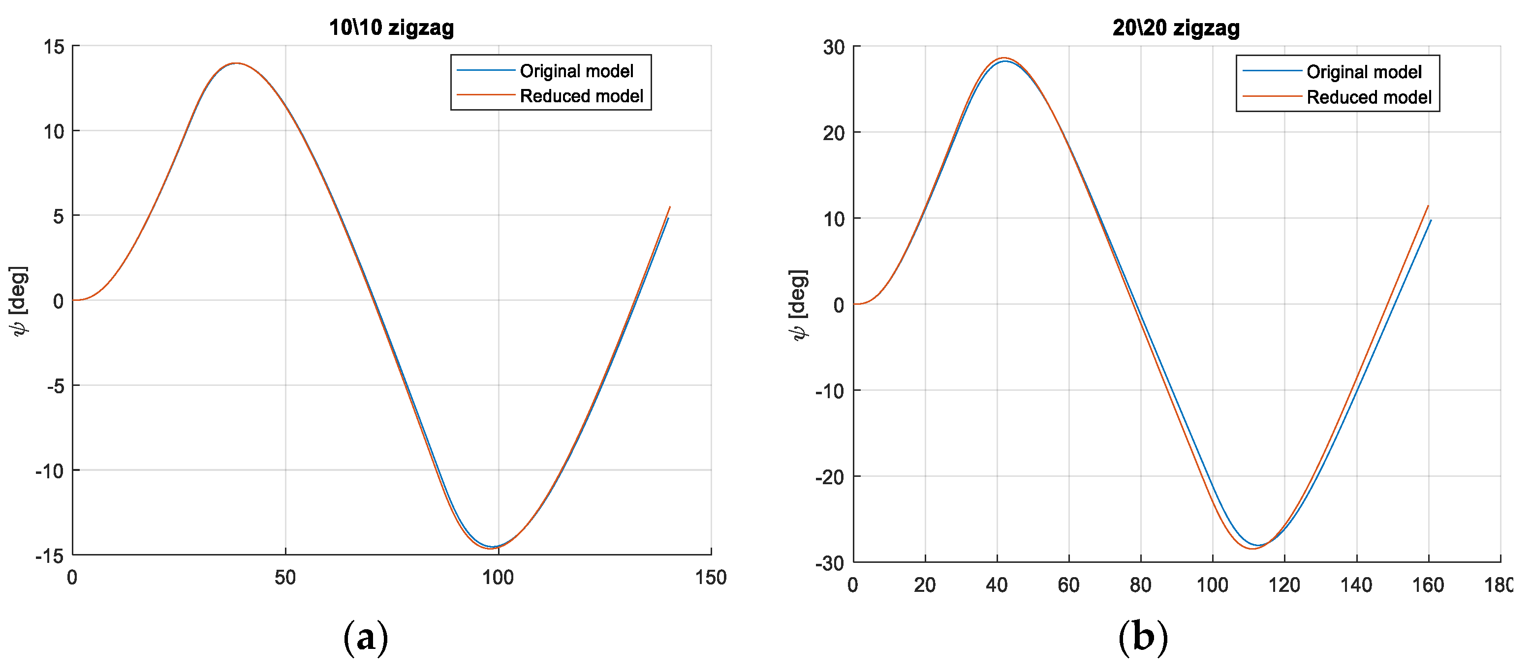
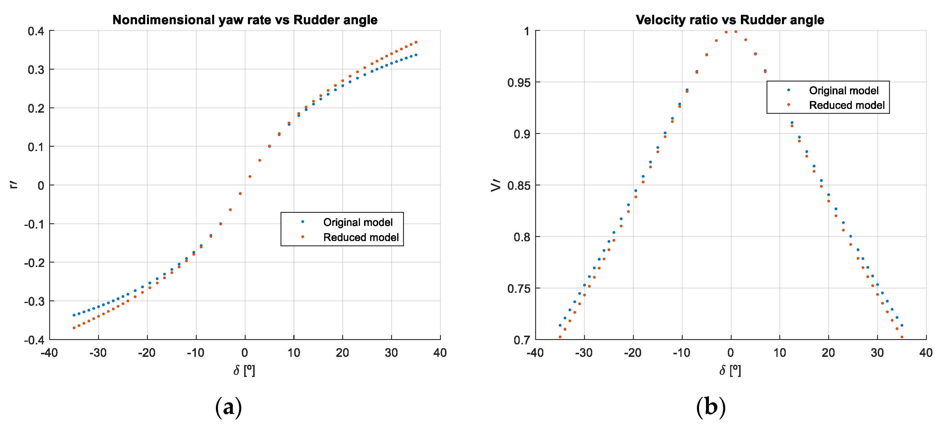
The comparison of simulation results obtained by the original and the simplified models showed the effectiveness of the sensitivity analysis for the model reduction task.

Future work could use these sensitivity analysis results to develop a consistent research strategy for system identification using data from full-scale trial tests, establishing a reasonable compromise between model completeness, computation time and parameter identifiability. In particular, the least influential parameters can be fixed using a priori information about their values, or even removed completely.

It must be emphasised that the manoeuvring mathematical model used in the present article corresponded to a ship with a high degree of inherent directional stability and moderate turning ability. Thus, while the results of the sensitivity analysis are applicable with considerable certainty to similar ship configurations, they should not be applied to vessels with highly different dynamic qualities, especially if these are characterised by some degree of directional instability. Such cases require special investigation.