1. Introduction
The word “
risk” first appeared in connection with the study of insurance companies
ruin in the framework of so-called “
collective risk” models, and measured by its probability (see for example H. Cramer [
1,
2]). Over the years, this concept received an expanded interpretation and began to be involved in various areas of human activity, such as reliability, busyness, environment, social sciences, etc. At the same time, the main attention of researchers was focused on the problems of a risk situation, connected with exploitation of complex objects, systems and processes, occurrence and development. In contrast to the risks of insurance companies this line of research has been called “
individual risk models”. For the practical study of such risks, a methodology for risk analysis has been proposed (see for example [
3]). This methodology is based on the so called
risk tree construction and analysis. This methodology includes: a comprehensive analysis of risks, their classification, construction of a risk tree and calculation of a structural function of a risk situation development, as well as calculation of the main characteristics of risks.
Remark 1. Originally, the idea of construction and using tree was used at BELL Labs in connection with reliability analysis of complex systems and was given the term fault tree. Further, as mentioned above, the idea of fault tree construction has found more and more wide applications, including risk analysis in different spheres of human activity: in business, biology, environment, etc. In this regard, the concept of a fault tree has received a more extended definition—an event tree. However, in this paper, which focuses on risk analysis, we will use the term risk tree instead of more general one—event tree.
One of the main problems in studying risks is the lack of information about the time of their occurrence and development, as well as the damages [
4] caused by these phenomena. To counter these problems, researches created various concepts of uncertainty. The variety in the interpretation of this notion relates to the fact that different authors are based on different concepts of “uncertainty”, recently formalized the following way:
(a)
randomness, which is investigated by probabilistic methods [
5],
(b)
subjective uncertainty, studied within the framework of subjective probabilities [
6],
(c)
fuzzy uncertainty [
7,
8] and
(d)
expert uncertainty [
9].
The investigations involving construction of risk trees are numerous, one of them is provided in [
10], where the construction of a risk tree is used in combination with HAZOP analysis (Hazard and Operability) and computational fluid dynamics simulations. In [
8] the fault tree was constructed from investigation reports of navigational accidents and then the occurrence probability of basic events was calculated using fuzzy set, the key influencing factors were determined. In [
11] a case study of leakage in submarine pipeline is discussed to demonstrate the proposed methodology combining fuzzy fault tree analysis and Bayesian network to obtain updated prior possibilities of basic events and top event of system fault tree when new information are available.
Since the presence of uncertainty in the initial information is an integral feature of real objects, sensitivity analysis attracts attention of researches. In [
12], new sensitivity measures in the global sensitivity analysis of failure probability are presented. The case studies compared sensitivity indices from four sensitivity measures in application to small values of failure probability. The conclusion is that the sensitivity ranking of the input variables is approximately the same from each sensitivity measure, but the proportions of the main and interaction effects differ significantly.
In multiple publications devoted to hazard analysis techniques [
13,
14,
15,
16], risk is considered as a combination of the probability of the failure event and the severity of its consequences. In complex technological systems with many risk events, determining their risk rating becomes essential. Mathematical modeling provides support in decision-making and requires the correct and complete specification of the initial data about the system.
In some of our work the problems of preventive maintenance optimization for the subsea pipeline monitoring system with respect to availability maximization in [
17] and with respect to cost-type criterion in [
18] has been considered. In [
19] it was proposed to use the risk tree as an assistant tool for the decision-maker. In [
20], the general principles of risk analysis with the help of a risk tree are applied to the real situation of a subsea pipeline monitoring system.
In this paper we follow to the concept of risk as a random phenomenon in Kolmogorov’s interpretation. From this point of view, any risk event can be considered as a member of a family of risk events forming a certain probability space . At that the scenario of risk occurrence and development can be represented as a two-dimensional random variable (r.v.) , where T is the time to the risk event A occurs, and X is a damage, associated with it. Accordingly, the risk tree can be considered as the probabilistic space of risk phenomenon construction.
Based on this approach in [
21] additional possibilities of event tree using for risk analysis were proposed. This approach, in addition to construction a risk tree, also includes loading it with data, calculating the risk structure function and main characteristics of risks, searching the most dangerous paths of the risk situations development with respect to different criteria, and analysing their sensitivity to the initial information.
The paper is organized as follows. In the next section the main ideas about risk tree construction and analysis will be proposed. Then in the
Section 3 one real-world example of an automated system for remote monitoring of underwater sections of the Dzhubga-Lazarevskoye—Sochi gas pipeline [
22] will be described in the framework of proposed approach. Finally in the
Section 4 the numerical study of risk tree based on proposed example will be presented. The paper concludes with directions for future work.
2. Methodology for Risk Trees Construction and Analysis
In this section the main steps of a risk tree construction and analysis will be presented. Most of up-to-date complex technical objects and systems have hierarchical structure. Accordingly, the development of risk situation associated with complex technical systems and processes imposes their hierarchical structure. Arising in the smallest parts of the system, a dangerous situation affects more and more parts of the system, in the end it affects the entire system. A hierarchical structure of a complex risk event can be visualized as a turned over tree-type graph.
Definition 1. A risk tree is a turned over tree-type graph, the root of which is a resulting risk event, its branches represent intermediate events of different levels, arcs show the connections between them, and leaves represent initial (original) risk events.
The example of such tree will be considered in details in
Section 3. For the complex risk events this procedure can be effectively organized by constructing risk sub-trees for each subsystem.
For representation of complex risk events the vector notation will be used. Denote the number of elementary risk event by vectors
, where
is the number of the risk event of the first level that leads to the main risk event,
is the number of the risk event of the second level that leads to the
risk event of the first level, etc.;
is the number of the elementary risk event of the
r-th level that leads to the event
, and
r is the hierarchy number level of considering elementary risk event (its rank), at that the ranks of different elementary risk events can be different.
1 The numbers of risk events of the
k-th level will be denoted by truncated vectors
, and the number of
j-th risk event of event with number
will be denoted by
. Appropriate to these notations the risk events with number
will be denoted as
. We denote structural variable of an event
by
, where
= 1, if an event
occurs and
= 0 otherwise.
For the risk tree construction the special notations for different type of risk events and connections between them (gates) have been proposed in [
3]. We use these notations for example description in the
Section 3 and its study in the
Section 4. Each gate corresponds to a certain structural function and based on them corresponding structural functions
for any event of any level
k (including the main one for
) can be found using rules of the type of gates (that is connected different events of the risk tree). Thus, the structural function for the
k-th level intermediate event with the last event
has the form
For the risk tree analysis we need in initial information that consists in distributions of random variables (r.v.’s) and :
cumulative distribution functions (c.d.f.’s) of time to the initial risk event occurrence and the damage connected with it
and c.d.f.’s of their spreading along the paths of the risk situation development,
The risk tree analysis involves risk structural functions and consists in calculating the main risk characteristics:
the c.d.f. of time before an event occurs;
the c.d.f. of corresponding damage ;
the survival function for intermediate and main risk events ;
the main and intermediate risk event probabilities of any risk event due to its j-th event;
the most dangerous paths of a risk situation development.
2
Based on given initial information and considered risk scenario the procedure for the c.d.f.’s of the risk event time occurrence and connected with it damage distributions looks as follows. Since each vector index
uniquely determines the original risk event, and a truncated vector
uniquely determines appropriate intermediate event, the times to their occurrence and corresponding them damages along the path to the risk event
have the form
Thus taking into account that the values
and
for event with number
along the way
j are the sum of values
and
in the event of
-th level
and additional values
,
along the path
j, it holds
Therefore their c.d.f.’s under the assumption of independence of the terms are calculated by convolution
Thus, the c.d.f. of time before any intermediate event
occurs that is equal to
can be calculated by following to the rule of the event structural function calculation as
Appropriate event survival function can be find as
For calculation of the c.d.f. of corresponding cumulative damage that is equal to
it is necessary to take into account that it depends on the path of risk event development, and accordingly to Formula (
4) equals
From here for corresponding c.d.f. of the damage value of
-th risk event it follows
Concerning the main and intermediate risk event probabilities
of
due to its
j-th event component it can be calculated as:
Using Formula (
7), we find the maximum risk event probabilities
and the number of subsystem
at which this maximum is reached.
Collecting these values together, we find for any
k the most dangerous path according to the maximum risk event probability criterion, including path for the entire system with
:
Appropriate calculations should fulfill beginning from the lowest level r up to the localization of the event including level for the main risk event.
Details of a risk tree construction will be shown in the next section for the risk tree construction for concrete example.
3. An Example: The Risk Tree Construction for a Underwater Gas Pipeline System Monitoring
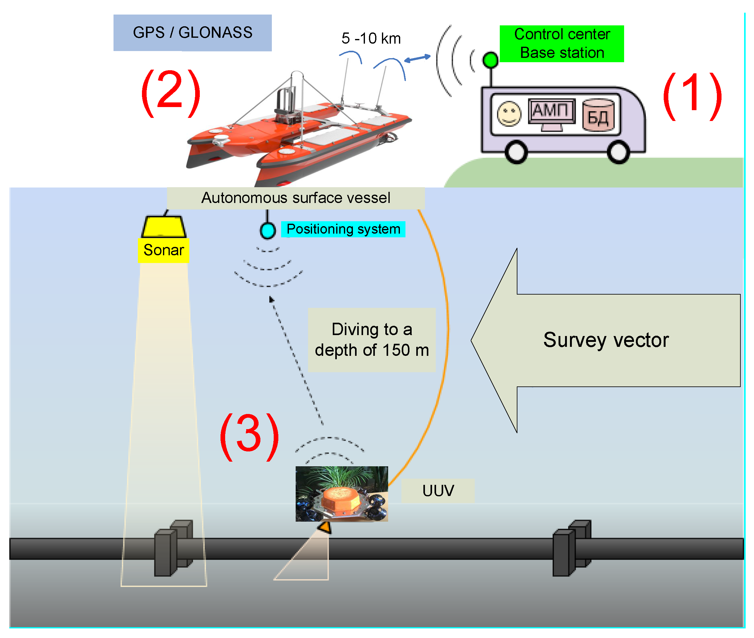
In up-to-day conditions, especially in connection with the explosion of the Nord Stream gas pipelines, it is of particular importance not only to constantly monitor the state of underwater pipelines, but also to organize their continuous protection from terrorist attacks. The problem of organization of protection has yet to be solved, and the scheme for organizing monitoring of the state of the coastal underwater pipeline is shown in
Figure 1. According to a similar scheme, monitoring of the Dzhubga-Lazarevskoye-Sochi gas pipeline is organized (see [
17]).
The aim of this section is to present a risk tree based on a real system of remote monitoring of underwater sections of the Dzhubga-Lazarevskoye-Sochi gas pipeline. The gas pipeline has been in operation since June 2011. The capacity of the gas pipeline is about 3.78 billion cubic meters of gas per year. The length of the underwater section is almost 160 km. The gas pipeline runs approximately 4.5 km from the waterfront. The sea depth reaches 80 m. The average service time is about 50 years, 11 years of service time have already passed, so it is necessary to monitor the condition of the pipeline for extending the service time.
The purpose of monitoring is to carry out a set of measures for an external survey of the offshore section of the gas pipeline to determine its technical condition, identifying the places of detected defects and providing video footage and relevant data for subsequent analysis to determine the causes of defects and assess the technical condition of the gas pipeline and its route. Visual inspection of underwater areas with fixation of video materials is carried out using a remote-controlled unmanned underwater vehicle (UUV) equipped with an HD video camera with appropriate lighting. UUV position determination is carried out using hydroacoustic positioning systems with an ultra-short base, which provide a relative error in measuring the vertical coordinates of the vehicle no more than 5% of the distance between it and UUV.
To perform bathymetric, sonar surveys, as well as to ensure visual surveys with UUVs the entire marine part of the gas pipeline, an autonomous surface vessel is needed, which meets the parameters prescribed by technical requirement specification. The vessel is equipped with hydrographic and geophysical systems.
Underwater sections of gas pipelines are a hazardous production facility. Timely detection of defects and their elimination removes the risks of disasters and damage to these objects. At the same time, the assessment of the performance, the calculation of the risk of failures of the hardware and software complex for the purpose of remote survey of the offshore sections of the gas pipeline using an UUV, is an important task.
In our numerical study we focus on the main devices of the system’s components and subsystems. As mentioned above in
Section 2 all subsystems and components will be denoted by vector indexes. At the same time for the simplicity appropriate risk events (which in the considered case coincide with their failures) will be denoted by the same vector indexes. Thus, following to description of our example for its risk tree construction we need distinguish three important subsystems (see
Figure 1):
(1)—onshore control center and wireless base station;
(2)—surface vessel, floating on the surface along the gas pipeline;
(3)—underwater vehicle (UUV) (see [
23]).
The main risk event is generated by the failure of the entire monitoring system.
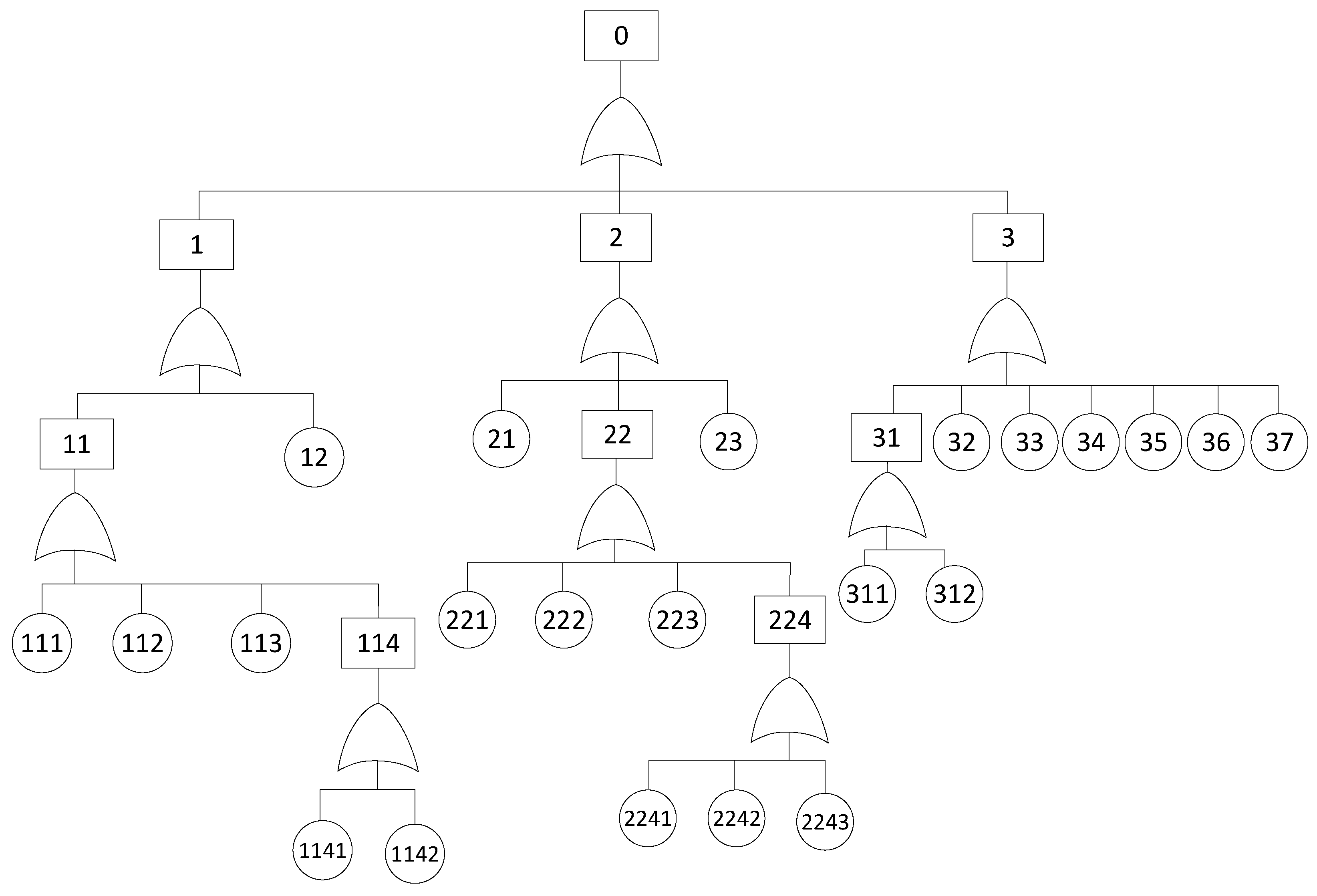
On the onshore control center and wireless base station (subsystem (1)) we highlight the following important events:
(11)—control module breakdown and
(12)—car breakdown.
Then we dive into the problem of event (11) and analyze why it could happen. There are four risk events:
(111)—personal computer breakdown with a built–in database (DB);
(112)—software does not work;
(113)—control tool does not work;
(114)—radio system breakdown.
The last event (114) can occur due to two events:
(1141)—network equipment breakdown or
(1142)—antenna breakdown.
The risk events that lead to the main one due to failure of the subsystem (2) are:
(21)—hydro echolocation system breakdown;
(22)—control module breakdown;
(23)—the battery got wet or discharged.
The risk event (22) contains sublevels:
(221)—navigation system breakdown;
(222)—local underwater positioning system breakdown;
(223)—radio system breakdown;
(224)—wire communication system for winch breakdown.
The last one can occurs due the following risk events:
(2241)—electric winch software does not work;
(2242)—neutral buoyancy cable broke;
(2243)—electric drive does not work.
The third subsystem is the most vulnerable, because the initial risk event occurrence time (EOT) under water is significantly reduced. We define the following risk events related to risk analysis in subsystem (3):
(31)—video system breakdown;
(32)—battery breakdown;
(33)—leaky housing;
(34)—control system breakdown;
(35)—any sensor breakdown, such as a depth gauge, gyroscope; compass, voltage sensor;
(36)—gripper breakdown;
(37)—motor drivers breakdown.
We need to say, that event (31) consists of two risk events:
(311)—camera breakdown and
(312)— lamps failure.
For the risk tree representation, we use the symbols of events and gates from [
3] (see
Appendix A). According to the methodology proposed in [
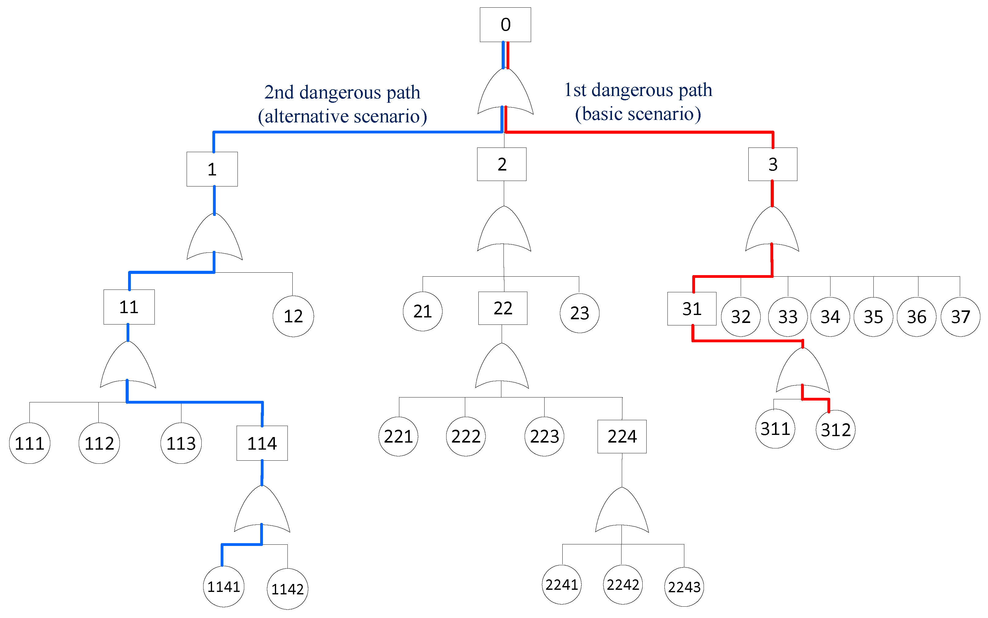
3], and based on the nomenclature above, a risk tree for the gas pipeline system monitoring has been constructed. It is shown in
Figure 2.
For the risk tree analysis, we need the initial information, which includes statistical data, expert estimates, manufacturer’s specifications, etc. We limited ourselves by analysis of the risk situation development in time only. Therefore, we omit the information about damages arising from any risk events. Moreover, we assume that there are no intermediate delays in the development of the risk situation. Thus, we need only the information about initial risk events occurrence. However, since it is impossible to obtain the c.d.f. of the initial risk event occurrence time (EOT), we limited ourselves by the mean EOT. Based on expert assessments, their values are presented in
Table 1, mean EOT are given in years.
Based on the methodology proposed in [
21] the main risk characteristics can be calculated with the help of structure functions, including c.d.f. of the time to the intermediate and the main risk event occurrence, the maximum risk event probability
of
risk event due to its
j-sub-event: see Formulas (
5)–(
8). The analysis of the sensitivity of the risk characteristics to the shape of the time to initial risk events occurrence and their coefficients of variations will be also under our attention.
4. Numerical Analysis of the Risk Tree for the Underwater Gas Pipeline System Monitoring
The purpose of this section is to test the proposed methodology using the example above, as well as to analyze the sensitivity of the risk characteristics of the main event to the type of the initial risk EOTs distribution and their coefficient of variation. In numerical experiments, we use Gnedenko-Weibull (GW), exponential and Gamma distributions for the leaves EOT. The parameters of all distributions in experiments are chosen such that their expectations coincide for different distributions with mean leaves EOT in
Table 1, while the coefficient of variation
takes different values in the interval
.
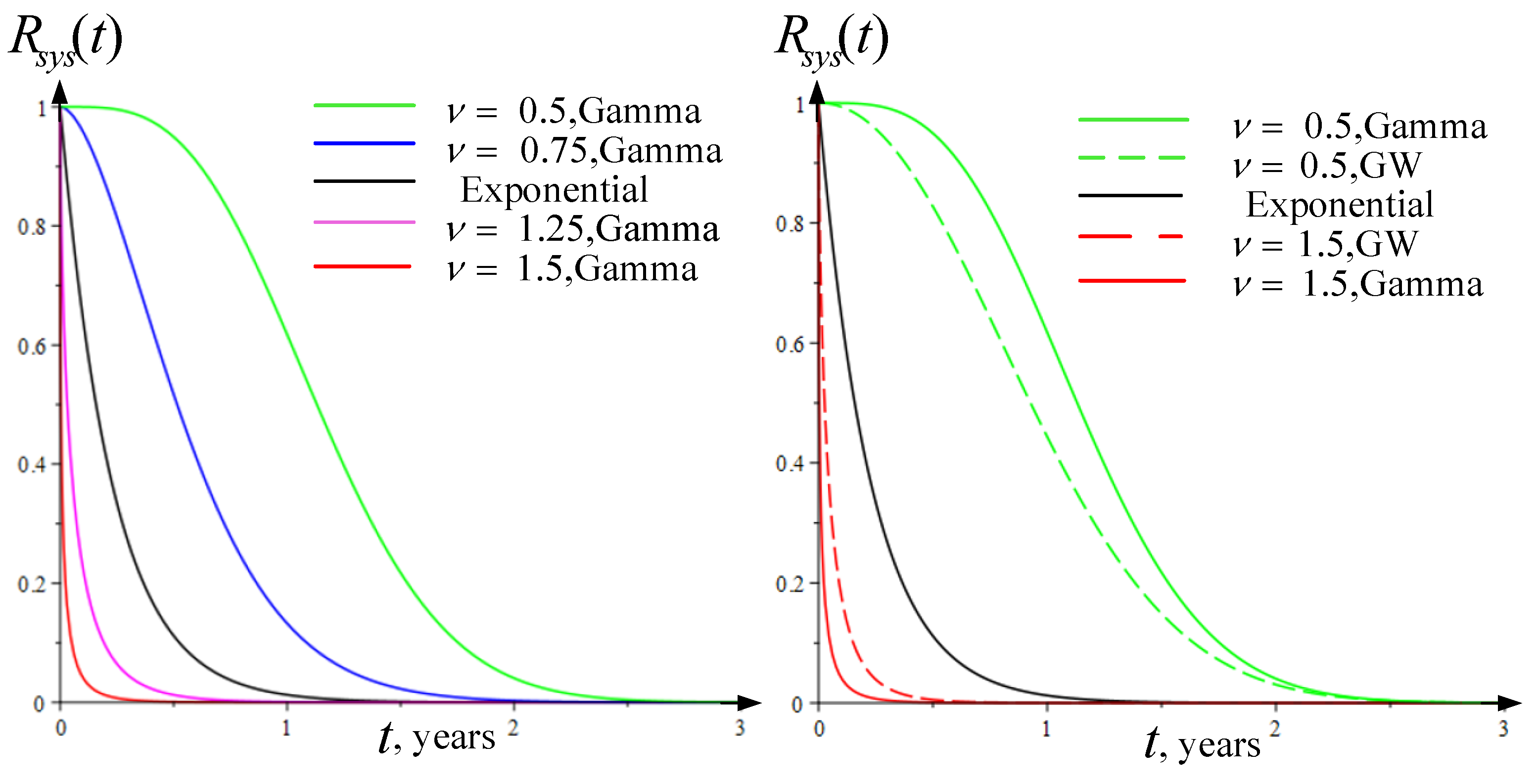
The picture below shows the graphs of the system reliability functions on a one-year time scale.
Figure 3 on the left shows the effect of the coefficient of variation on the system reliability function for the Gamma distribution for all elementary events. System reliability decreases with increasing coefficient of variation, this is especially noticeable for
.
Figure 3 on the right presents the influence of the shape of the distribution. Reliability function for Gamma distribution deviates greater from exponential one than Gnedenko-Weibull distribution. The difference between the reliability functions calculated for
is about 0.17 in case
.
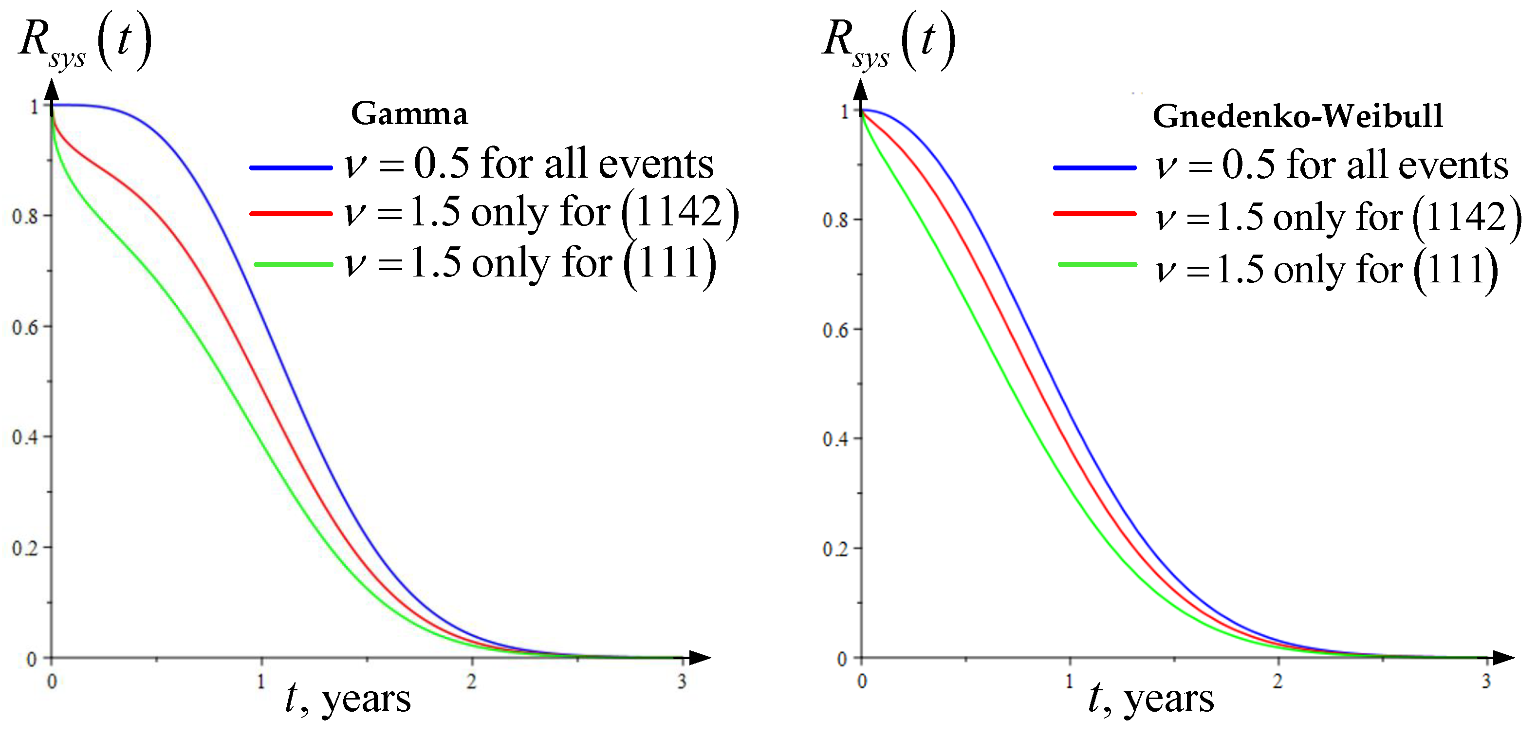
In real life, all EOT have different coefficients of variation. Our next experiment demonstrates how just one event with a high coefficient of variation changes the reliability function of the entire system. In
Figure 4 on the left, all EOTs follow Gamma distribution with
, except for one event in the first subsystem. In
Figure 4 on the right, all EOTs follow GW distribution with
, except for the same event. Two events were chosen for sensitivity analysis: an antenna breakdown (1142) with a mean EOT of 20 years and a personal computer breakdown (111) with a mean EOT of 5 years. Note that an increasing the coefficient of variation for an event with a shorter mean EOT (green curves) affects reliability functions more strongly than for an event with a longer mean EOT (red curves). Changing the coefficient of variation from 0.5 to 1.5 for only one event significantly affects the reliability function, as shown in
Figure 4.
Next step of the risk analysis consists in calculating the probabilities of risk event occurrence and in determining the most dangerous paths of a risk situation development according to the criterion of risk event probability maximization. The numerical experiments are described below. In the first experiment (a basic scenario) all leaf EOTs follow the Gamma distribution, the coefficient of variation for all EOTs .
The probabilities of risk events and the most dangerous paths calculated according to Formulas (
7)–(
9) starting with leaf events equal
This path is shown in
Figure 5 with bold red line. Event (312) has mean EOT of 2 years (the minimum mean value in monitoring system of all events), so this dangerous path starting from event
for the basic scenario is really justified, since it includes the most vulnerable event of the system. For comparison, we also calculate the probabilities of system failure due to the failure of its subsystems (1) and (2)
.
For the second experiment, the coefficient of variation
is changed to
only for one event (1142) (antenna failure) with a mean EOT of 20 years. The input data for other events is identical to the basic scenario. The most dangerous path hasn’t changed, but the corresponding probabilities has changed:
However, we can offer the decision-maker an alternative dangerous path starting with event
:
Note that the alternative path does not start from leaf event (1142) with a coefficient of variation
, but from a neighboring event (1141), apparently since its mean EOT is only 3 years, which is significantly less than the mean EOT of the event (1142)–20 years. We see, that changing the coefficient of variation of event (1142) adds a second dangerous path to the system, which is shown in
Figure 5 with blue color.
Next series of experiments involves the mixture of Gamma and GW distributions, the results of which are shown in
Table 2. For the first experiment (I), we estimate the risk event probability
of system (0) due to the failure of subsystems (1), (2) and (3), each leaf EOT has a coefficient of variation
. The distributions at the lower levels are Gamma, at the next level–GW, then again we take Gamma, etc. System failure is more likely due to subsystem (3), the greatest failure probability is given in bold. The results are shown in the first row of the
Table 2.
For the second experiment (II), we change the EOT distribution for only one leaf event (1141) and calculate again risk event probabilities
. The initial data of the I and II experiments are close to each other, we can conclude that for the model under consideration changing of the distribution of EOT for one event has small effect on the subsystems risk event probabilities. The subsystem (3) also has the highest probability of failure in this case. The results are presented in the second row of the
Table 2.
In the third experiment (III), EOT of event (1141) has the same distribution as in the first one, but the coefficient of variation , the other parameters of EOT distributions coincide with first experiment. Subsystem (1) has the highest risk event probability now. We conclude that the initial data characteristics can significantly influence the technological risks prediction and the construction of risk paths.
Table 3 shows the quantiles of reliability functions for Gamma and GW distributions of EOTs. Four scenarios are represented: (I)
v = 0.5 for all events as a basic scenario; (II)
v = 1.5 only for one event (1142) (antenna failure) with a mean EOT of 20 years or (III) event (111) (PC failure) with a mean EOT of 5 years as a possible scenario; (IV)
v = 1.5 for all events as an extreme scenario. The changing of the coefficient of variation dramatically affects the estimation of the quantiles of the reliability functions.
All our experiments confirm the very popular among engineers opinion that for construction a reliable system, the equally reliable components should be used.
5. Conclusions and the Further Research
The paper proposes the risk analysis methodology that makes it possible modeling the time to risk events occurrence, and the damage associated with it, as well as the risk situation development from the initial event up to the main one. Moreover, the presented methodology allows the researcher to find the most dangerous paths of a risk situation development with respect to various criteria, which constitutes the novelty of the work.
The key issue is the quality of initial information. Mathematical models require the information about distributions of risk EOT and associated with them damages as well as their parameters. The uncertainty in this information can lead to erroneous conclusions and wrong decisions. Collection and analysis of the initial information about risk situations occurrence and development will improve the quality of decision making.
The proposed methodology has been tested on a real-world example using a number of numerical experiments. Unfortunately, the lack of information necessary for this analysis did not allow us to provide the full study and we limited ourselves with only investigation of risk situation occurrence and development in time.
Numerical experiments have shown a significant sensitivity of the main and intermediate risk events characteristics to the shape of distributions of the initial risk events occurrence times as well as to the value of their coefficient of variation.
Thus, as a novelty, the work shows the importance of preparing and analyzing the initial information concerning the distributions and their parameters of the risk situation occurrence and development. Along with a deeper analysis of the sensitivity of scenarios for the development of a risk situation, statistical analysis of the initial information about risks should be considered as the most important direction in the development of the theory of individual risks in the future.


 ,
, 


