Development and Validation of Accumulation Term (Distributed and/or Point Source) in a Finite Element Hydrodynamic Model

Abstract

During tropical storms, precipitation and associated rainfall-runoff can lead to significant flooding, in both the upland and coastal areas. Flooding in coastal areas is compounded by the storm surge. Several hurricanes in recent history have exhibited the destructive force of compound flooding due to precipitation, rainfall-runoff, storm surge and waves. In previous work, various coupled modeling systems have been developed to model total water levels (defined as tides, waves, surge, and rainfall-runoff) for tropical storms. The existing coupled system utilizes a hydrologic model in the upland areas of the domain to capture the precipitation and rainfall-runoff associated with the storms; however, in the coastal areas the precipitation and rainfall-runoff is not captured. Herein a source/sink term is incorporated within the hydrodynamic model itself to capture precipitation and rainfall-runoff over the already inundated coastal areas. The new algorithm is verified for several idealized test cases, and then it is applied to Hurricane Irene. Validation indicates that the new methodology is comparable to the existing river flux forcing under most conditions and allows for the addition of streamflows due to overland runoff, as well as the actual precipitation itself.

1. Introduction

Over the last several years, it has become evident that devastating flooding along coastal regions during tropical storms or rainfall-intense storms (i.e., Hurricanes Harvey, Irma and Florence [1,2,3]) is often caused by precipitation and upland rainfall-runoff (additional streamflow or overland flow due only to precipitation; does not include groundwater flows or interflows) [4]. Many tropical storms have led to flooding within the areas that they make landfall; however, Hurricane Harvey had the most rainfall associated with it, more than from any other tropical cyclone event that has occurred within recorded rainfall records of the United States [1]. The rainfall associated with the storm was significantly above the 100-year rainfall event for the Houston area and many other regions of southeastern Texas. In fact, Blake and Zelinsky [1] determined that the rainfall over most of the areas of southeastern Texas had a “less than a 1-in-1000 (0.1%) chance of occurring in any given year (e.g., a 1000-year or greater flood)”. The rainfall-runoff produced from the storms caused many of the rivers and creeks in these areas to exceed their banks; in fact, in Harris County alone, there were “9 out of the 19 official river gauges” that showed record flood stages [1]. These record flood stages led to catastrophic flooding in the urban areas of Houston and Beaumont. Furthermore, the significant rainfall led to issues with some of the dams and spillways in the Houston area reaching the reservoir capacity and threatening failure; thus, some of the water in these reservoirs was intentionally released leading to exacerbated flooding in many of the areas downstream of these reservoirs. There were 68 fatalities caused by Hurricane Harvey within Texas and it was determined that all but three of these deaths resulted from freshwater flooding [1]. Similarly, Hurricane Irma caused record-breaking flooding in Jacksonville, Florida due to the combined effect of both rainfall-runoff and storm surge, which led to “one of the worst flooding events in the city’s 225+ year history” [2]. Finally, the freshwater flooding from rainfall-runoff during both Hurricanes Florence and Matthew caused significant flooding within the riverine areas of the Tar, Cape Fear and Neuse Rivers in North Carolina, with rainfall totals of 48 cm occurring over portions of North Carolina during Matthew [5].

Due to these storms and several others, it has become evident that to capture the combined effects of storm surge and rainfall-runoff a dynamic model is needed. Many of the areas discussed above are considered part of the coastal riverine zone or the coastal transition zone which is not captured by most operational models. In the operational framework that provides official guidance and forecasts for flooding, the hydrological models predict riverine flooding in rural and urban areas for the inland areas, while another set of hydrodynamic models predict coastal flooding due to storm surge, but these models are run independently from each other. Thus, capturing the riverine and rain flooding in this coastal transition zone, particularly in urban areas, represents a service gap for the National Weather Service (NWS) [6,7,8]. In fact, NOAA’s Water Initiative is looking to develop, demonstrate and implement a way of obtaining the compound flooding that occurs within the dynamic coastal zone [9]. Furthermore, this dynamic coastal zone is also of interest to the Department of Homeland Security (DHS) and the Federal Emergency Management Agency (FEMA). In particular, FEMA flood maps treat the risk assessment for each hazard as independent in coastal areas: one map for flooding that might occur based on upland runoff and one map for flooding that might occur due to storm surge associated with landfalling hurricanes or tropical storms [10].

In the last fifteen years, researchers have developed several different coupled modeling systems that bring in the riverine flows within the upland areas of a coastal domain. These systems employ various methodologies to capture the riverine flows and flooding that occur in the upland areas, including: incorporation of data from the United States Geological Survey (USGS) real-time gauging stations [11,12,13], input as a riverine boundary condition with information from a hydrology model [14,15,16], through more complicated 3D implementations that consider baroclinic changes due to evaporation and transpiration [17,18,19], and by incorporating the hydrologic or hydraulic models with gridded techniques within the hydrodynamic model [20]. However, many of these systems do not include the surface runoff or rainfall that occurs in the coastal transition zone below where the connection to the upland rivers occurs [7,21], thus missing a portion of the water level increases that can occur in this region.

The hydrodynamic model utilized within this manuscript, called ADCIRC (ADvanced CIRCulation) [22], currently uses a riverine boundary condition with streamflow information input from a separate hydrology model. Within this framework, ADCIRC has been successfully coupled to hydrologic models and applied in the study of both hindcasts of historical storms [6,7] and future climate predictions [23]. While this does introduce the main upland riverine streamflows into the coastal zone, it does not capture the rainfall-runoff that occurs downstream of those connections, which can lead to missing surface runoff (lateral inflows), nor does it capture the actual precipitation in the coastal areas. This existing river flux boundary condition methodology within ADCIRC requires that the model be refined with the channels clearly defined all the way to the model boundary with the surrounding floodplains similarly refined in order to capture flooding from the channel and satisfy smooth element transitions. This is time consuming for model development, as well as simulation time, as the small grid resolutions necessary for this refinement will necessarily restrict the maximum stable time step for the model (due to the Courant Friedrichs Lewy condition [24]). It is also restrictive, in that only riverine features that intersect the model boundary can have streamflows applied.

Herein we implement a new source/sink term into the ADCIRC governing equations, which allows the introduction of both the precipitation over the coastal zone and lateral inflows for additional riverine contributions. In this implementation, precipitation is only added over the already wet areas of the domain; however, other researchers are exploring the implementation of a routing scheme within the hydrodynamic model to bring in the precipitation that occurs over the entire coastal zone [25]. However, these routing implementations could significantly impact the computational time required and reduce the effectiveness of the model as a real-time predictive tool. By using the proposed point source (lateral inflow) methodology to incorporate inland hydrology, it is possible to include streamflows from any hydrologic feature that ends in the wet portion of the domain even if it is not refined to the mesh boundary. The “wet domain” requirement forces hydrologic input to only be added to regions of the model domain that already contain water, since the current formulation of the hydrodynamic equations does not allow for routing of water across the dry elements (hydrologic modeling). In this way, rivers and tributaries that are smaller than the grid resolution of the hydrodynamic model, but which can produce significant streamflows during extreme weather events, can still be incorporated.

Throughout this paper, the term “wet” or “wet domain” is used to refer to all nodes within the model domain that satisfy at least one of these three criteria: (1) node has positive bathymetry indicating that it lies in water, (2) node has been inundated in the course of the simulation and flagged as wet in the internal wet/dry algorithm, or (3) node lies above MSL but is within a river channel and has been given an initial water elevation (these nodes may become dry if input streamflows become too low during the course of the simulation).

The layout of the paper is as follows: Section 2 discusses the addition of the source/sink term within the ADCIRC model governing equations and presents the methodology for obtaining streamflow information from the selected hydrology model, National Water Model (NWM [26,27]) for the lateral inflows; Section 3 presents ideal model results to verify the implementation of the new source/sink term; Section 4 presents applications and validation of the new methodology for Hurricane Irene in the North Carolina area; and Section 5 summarizes the results and provides conclusions and possible future work.

2. Methodology

2.1. Addition of a Source/Sink Term—Used for Both Distributed and Point Sources

In order to add a new source/sink term within the wet areas of the coastal zone, it is necessary to follow the development of the governing equations for the Generalized Wave Continuity Equation (GWCE)-based model, ADCIRC [22,28]. Namely, the source term is added directly to the conservation of mass, or continuity equation, and then a new equation for the GWCE is derived. The continuity equation with the additional source/sink term added to the right-side is given in Equation (1)

$$L\equiv \frac{\partial \zeta }{\partial t}+\nabla ·\left(Hv\right)=I$$

(1)

where $\zeta$ is the elevation of water surface above the datum; H is the total fluid depth, given by $H=h+\zeta$ with h for the bathymetry; t is time; $v$ is the velocity of the fluid in both the x- and y-directions, and I is the rate of the new source/sink term (right-side is zero otherwise). This source/sink term can be utilized for different information, e.g., precipitation or lateral inflows within the riverine system that are beyond the grid resolution utilized in the area. This is an important point, as the current ADCIRC formulation requires that riverine flows be added at the mesh boundary using the flux boundary condition and that the riverine channel system be resolved all the way to the edge of the model boundary, which requires the addition of many additional nodes in the finite element (FE) representation (and necessarily a smaller time step).

ADCIRC utilizes the GWCE instead of the primitive form of the continuity equation to eliminate the spurious modes that enter into the results due to the short wave ($2\Delta x$) noise that can appear in the FE scheme [29,30,31]. Kinnmark [28] proved the mathematical equivalency between the GWCE and the primitive continuity equation, provided that two conditions are met: (1) the numerical parameter, ${\tau }_0$ (sometimes referred to as G), is greater than zero; and (2) the initial condition for the partial differential equation satisfies continuity, which is met by spinning up the model from a cold start. The GWCE is given below in Equation (2)

$$W^G\equiv \frac{\partial L}{\partial t}+{\tau }_{0}L-\nabla ·M^C=0$$

(2)

where ${\tau }_0$ is a numerical parameter, which allows for the equation to vary from the pure wave form (${\tau }_0\to 0$) to the primitive form of the equation (${\tau }_0\to \infty$), L is the continuity equation (given in Equation (1)) and $M^C$ is the conservative form of the momentum equation (given in Equation (3)).

$$M^C\equiv \frac{\partial \left(Hv\right)}{\partial t}+\nabla ·\left(Hvv\right)+\tau Hv+\mathrm{H}f\times v+H\nabla \left[\frac{p_a}{\rho }+g\left(\zeta -\alpha \eta \right)\right]-A-\frac{1}{\rho }\nabla ·\left(HT\right)=0$$

(3)

Here $\tau$ is the bottom friction parameter, $f$ is the Coriolis parameter, $p_a$ is the atmospheric pressure, $\rho$ is density, $g$ is gravity, $\alpha$ is the Earth elasticity factor, $\eta$ is the Newtonian equilibrium tidal potential, $A$ is the atmospheric force and $T$ is macroscopic stress tensor (all equation variables use consistent metric units: meters for space and seconds for time).

Using the continuity equation in its original form and bringing in the conservative momentum equation, Kinnmark [28] developed the original form of the GWCE shown in the expanded form below:

$$W^G\equiv \frac{{\partial }^2\zeta }{\partial t^2}+\frac{\partial }{\partial t}\left(\nabla ·\left(Hv\right)\right)+{\tau }_0\frac{\partial \zeta }{\partial t}+{\tau }_0\nabla ·\left(Hv\right)-\nabla ·M^C$$

(4)

Now utilizing the modified continuity equation presented in Equation (1) and substituting into the GWCE given in Equation (2), a new formulation of the GWCE with the source/sink term additions is given below:

$$W^G\equiv \frac{{\partial }^2\zeta }{\partial t^2}+\frac{\partial }{\partial t}\left(\nabla ·\left(Hv\right)\right)-\frac{\partial I}{\partial t}+{\tau }_0\frac{\partial \zeta }{\partial t}+{\tau }_0\nabla ·\left(Hv\right)-{\tau }_{0}I-\nabla ·M^C$$

(5)

There are two new terms added to the GWCE due to the addition of the source/sink term to the continuity equation: $\partial I/\partial t$ and ${\tau }_{0}I$. These two terms are evaluated explicitly in the temporal discretization by incorporating the present and past values for the $\partial I/\partial t$ term while the ${\tau }_0$ term is only evaluated at the present time.

For the distributed sources, precipitation intensities, or rates, are input directly into ADCIRC as structured data sets with rates specified at each point in the structure (I, mm/hr). Precipitation intensities can be obtained from several sources including: Quantitative Precipitation Estimations or Forecasts from meteorological models (QPE/QPF [32,33]), Multi-Radar/Multi-Sensor (MRMS [34]) data, precipitation from hydrologic models [26,35] and numerical precipitation models such as the parametric rainfall model (P-CLIPER [36]). In this way, precipitation intensities can be included within ADCIRC at both the basin-scale and regional-scale.

Meanwhile, lateral inflows or point sources are input into the ADCIRC model as streamflows (Q, m³/s) with given locations. In the instances when the location is provided in longitude and latitude, ADCIRC internally locates the nearest node and converts the streamflow into an intensity using the wetted elemental area surrounding the point. Figure 1 shows an example of this. Lateral inflows can be obtained from any hydrologic model including: the National Water Model (NWM [26]), Ensemble Framework For Flash Flood Forecasting (EF5 [35]), Hydrologic Engineering Center – Hydrological Modeling System (HEC-HMS [37])) or from actual streamflow data provided at US Geological Survey (USGS) gauge locations [38] or other data sources.

Finally, nodal attributes within ADCIRC must be correctly specified for any riverine reaches that lie above mean sea level, as the defaults assigned during mesh creation would be assigned “land” values instead of “water” values given the bathymetry. More detail about this can be found in [39]. Note that the wet/dry status of each node in the domain changes throughout the length of the simulation and the new source terms (precipitation and lateral inflows) are automatically activated and deactivated based on this status. For this study, we are not examining the additional effects of waves so these are not true “total water levels.” However, now that the methodology is in place, coupled ADCIRC and SWAN [40] runs with precipitation and inland hydrology should be easily facilitated.

2.2. Procedures to Extract Streamflows from the National Water Model

Inclusion of the lateral source term requires that the location of the streamflow input be known, along with the magnitude of the streamflow itself. In order to incorporate lateral inflows for the riverine areas in this manner, a methodology for extracting location and streamflow from the hydrology model is necessary. For this study, the National Water Model (NWM) is utilized as the source for all hydrology input. The NWM is a hydrologic model that simulates streamflow over the entire continental United States (CONUS). There are currently about 2.7 million streamflow output points provided by the NWM for several different forecast ranges [27]. Coupling the NWM streamflows to ADCIRC for hurricanes and heavy rain events will allow ADCIRC to include streamflows from upstream reaches and more accurately capture the water elevation due to most aspects of the storm: hurricane storm surge, rainfall, and riverine flow. Herein, a “soft” one-way coupling is utilized whereby streamflows from the NWM are input into ADCIRC via file transfer (hereafter referred to simply as IO).

For any study area, it is first necessary to preprocess the NWM network to select only those features that end within the wet domain for the region of interest (it is not feasible either computationally or for IO to attempt to use all 2.7 million extraction points when most are beyond the scope of a particular study domain). Additionally, the floodplain region of a model is typically reduced to a region of interest rather than being CONUS-wide since the addition of the floodplain requires higher resolution and necessitates more computational cost [41]. Although recent additions to the Global Extratropical Surge and Tide Operational Forecast System (ESTOFS) ADCIRC model core [41] incorporates floodplains for the entire coastal region, it is still recommended that study specific regions of interest should be used for the selection and incorporation of NWM features to optimize performance.

A collection of preprocessing tools was created to facilitate the selection of the NWM stream network endpoints (hereafter referred to as NWM features) that end within the expected wet domain, which includes all wet nodes previously defined in the introduction. For the selection process used herein, a separate model domain of only wet nodes (e.g., only ocean, estuary, and riverine elements) was extracted from the full model domain, but other polygon search methods could also be developed. Details about the search methods and selection process can be found in [39]; herein, only the criteria used during the selection process are provided.

While the implementation within ADCIRC internally removes any features that end on the floodplain, a reduction of the total number of features is desirable for IO purposes. Therefore, only NWM features that end in the wet domain should be selected. Additionally, it is necessary to ensure that only one NWM feature for a given hydrologic feature is included in the implementation, otherwise multiple reaches of the same river may be input into ADCIRC resulting in unrealistically high water levels and “double (or higher) counting” of the streamflow. Within the methodology presented herein, the wet domain mesh aids in this process by providing a delineation of the water features themselves, which would not be clear from the full floodplain model itself: water elements are not simply the elements with bathymetry below sea level since most riverine features follow the surrounding topography and have depths above sea level. Given these constraints, the following criteria are used to select NWM features:

• The feature must end in the wet domain (reduction for IO purposes).
• The feature may not also begin in or “near” the wet domain (remove redundant features and find the uppermost reach of a river/stream).
• If a feature ends “near” the wet domain, further visual quality control must be conducted to determine if it should be added. This is necessary because the coarser resolution of the NWM stream network occasionally results in features being misaligned with the ADCIRC model water representation and automated procedures for comparing the NWM feature outlet to the ADCIRC water domain will not correctly identify all features that should be included. “Nearness” is defined by a user specified buffer (given in meters) and should be smaller than the typical element size in the upland rivers.

After the NWM features (to be included) are found, the final step is to create the ADCIRC model IO files by extracting streamflows from the archived reanalysis data [27] for those found features.

3. Verification of Methodology

The new source terms are evaluated with several idealized cases using both constant and temporally and spatially varying precipitation fields, as well as idealized applications of the point source implementation for lateral streamflows. For all ideal tests, the model domain consists of a 10km square region with a spatial resolution of 250m in both the x and y directions.

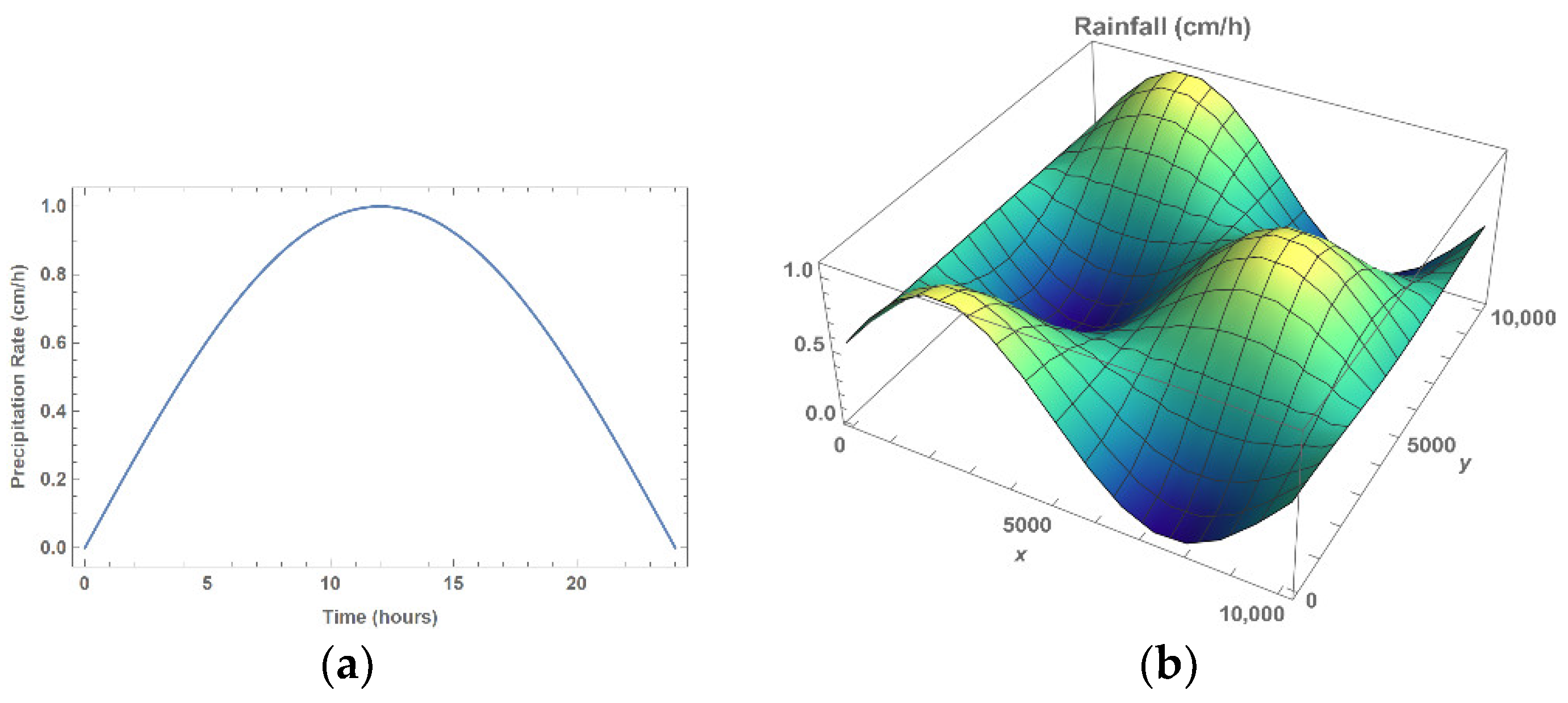
3.1. Idealized Test Cases—Distributed Sources (Precipitation)

For precipitation testing, the model domain is defined by a flat bottom with constant bathymetry of 20 m (z direction) and land boundaries on all four sides, i.e., a “bathtub” with no outside forcing except for the precipitation input. Four precipitation intensity scenarios are examined: a constant forcing of 1 cm/h over the entire domain for one full day, temporal varying intensities that vary sinusoidally from 0 cm/h to 1 cm/h and reach the peak at half a day and then return to zero (the same rate is applied over the entire domain), spatial varying intensities that vary sinusoidally in both spatial directions with a maximum rate of 1.08 cm/h and are constant in time and finally a spatial and temporal variation in intensity that linearly scales the spatially varying rate from zero to one at twelve hours and back to zero at twenty-four hours. Figure 2 presents the temporally varying and spatially varying precipitation intensities; for the spatial and temporal variation, panel b is just scaled by a factor ranging from zero to one.

For these idealized test cases, the methodology is verified using volume calculations, where the volume of applied rainfall is found by taking the area under the curve for the idealized rainfall. This value is then normalized by the cross-sectional area of the domain (converting it to an expected water elevation) and compared to the model results, where the “average” water surface elevation (WSE) is determined from the elemental change in the elevations normalized by the area of the domain. To determine the average water surface elevation for the final model output, the following equation is used:

$$\mathrm{Average} \mathrm{WSE}=\frac{1}{{10}^{8}sq m}{\displaystyle \sum }_{i=1}^{ne}{A}_i{\overline{\zeta }}_i$$

(6)

where $A_i$ is the area of the element (m²), ${\overline{\zeta }}_i$ is the average of the elevation changes within the element (m) and $ne$ are the number of elements within the domain.

Table 1. Comparison of water surface elevations for idealized rainfall tests cases with constant bathymetry.

	Expected WSE Due to Rainfall (cm)	Modeled WSE (cm)
Constant	24.00	23.99
Spatial	12.96	12.95
Temporal	15.29	15.29
Spatial and Temporal	6.48	6.48

shows a comparison of the water surface elevations from these idealized test cases. Results show that the addition of the source/sink term for the precipitation as a distributed source produces similar water surface elevations as the applied rainfall, indicating that the distributed source conserves mass and is producing consistent results. It should be noted that varying bathymetries (one was a sloped bathymetry with a 3 m to 100 m depth across the domain) were examined with these same rainfall intensities and the results indicated similar consistency in the model.

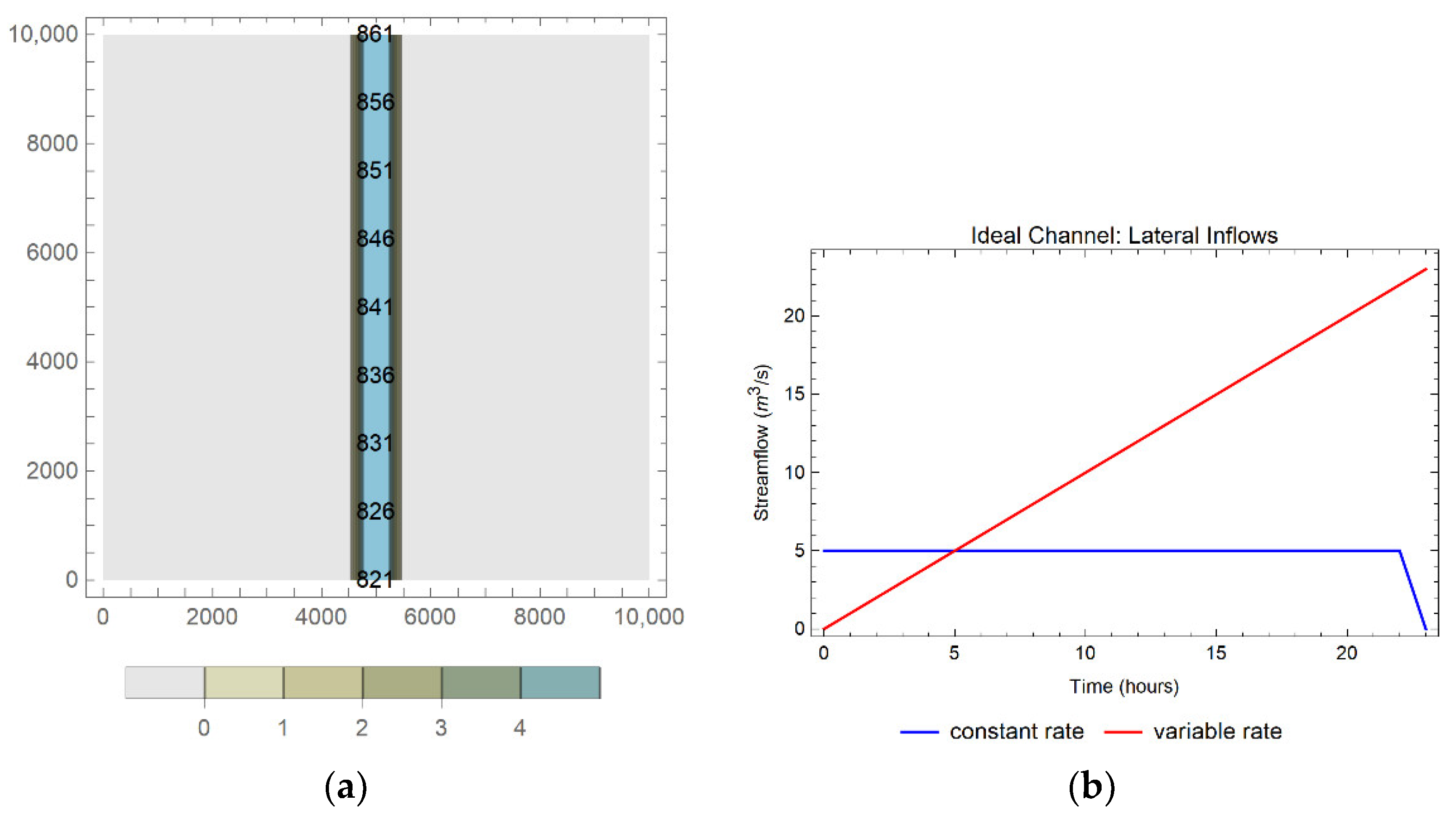
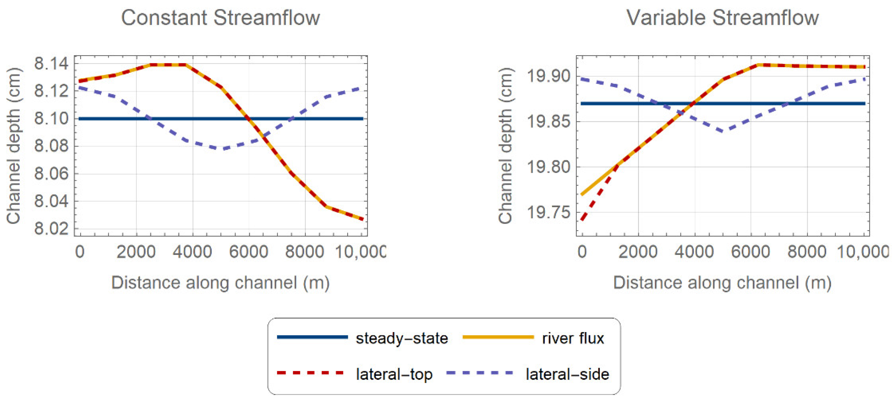
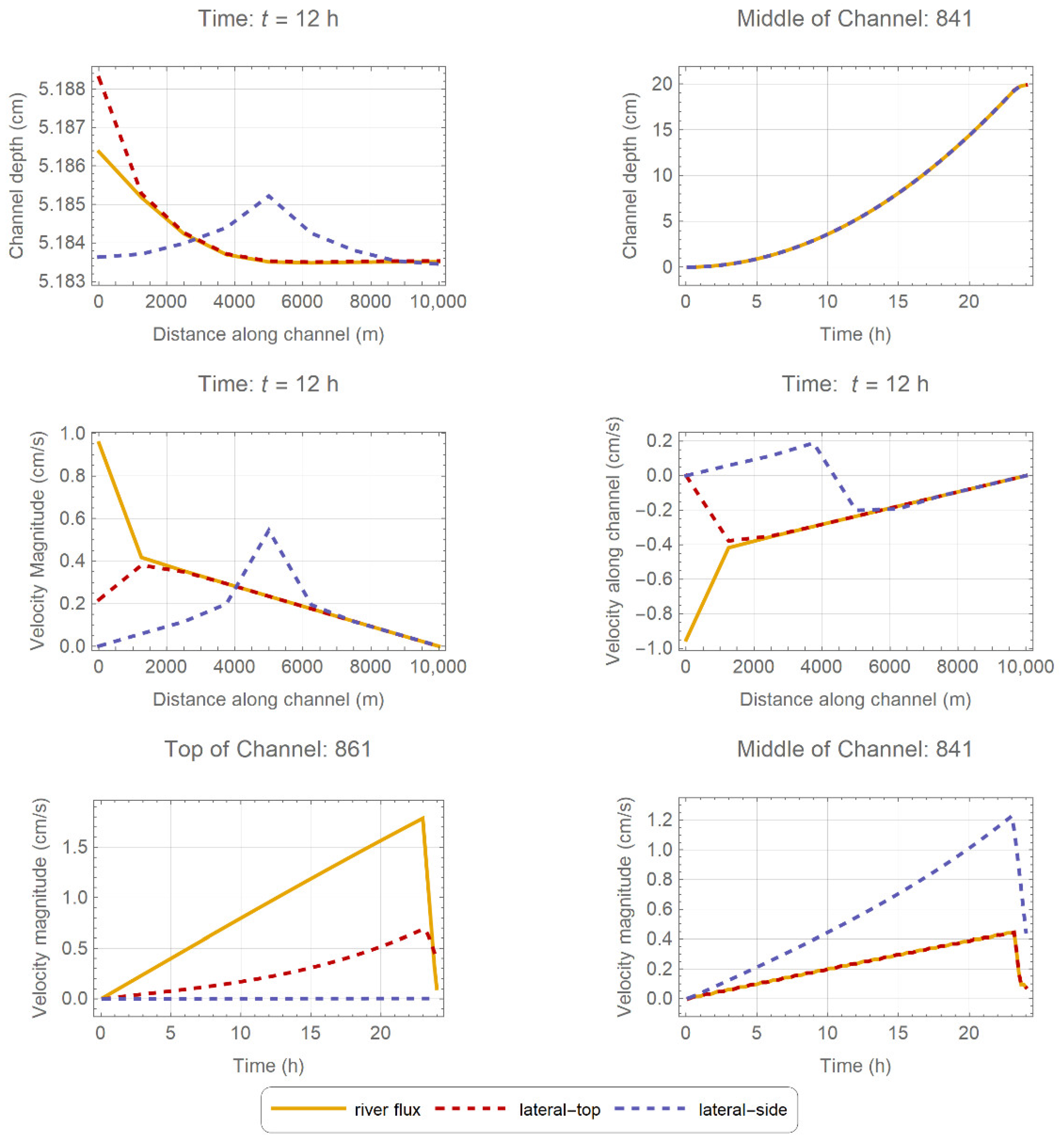
3.2. Idealized Test Cases—Point Source (Lateral Inflows) versus Boundary Flux

In order to test the source/sink term with point source or lateral inflows, an idealized channel with a constant depth (and surrounded by a floodplain) is used. The channel is two elements across and runs 5 m deep (rectangular cross-section) with the surrounding floodplain set at 1 m above mean sea level (MSL). The boundaries of the domain are closed so that all of the added water should remain in the channel. Figure 3 shows the idealized channel domain along with input for the different streamflow scenarios examined. With this idealized channel, two different streamflows will be utilized: a constant flowrate of 5 m³/s and a variable flowrate that varies linearly from 0 to 23 m³/s—both applied over one full day. For the constant rate test, the streamflow reverts to zero at twenty-three hours in order to compare steady-state timing behavior. Additionally, two input locations for the addition of streamflows are presented herein: the upper end of the channel at the boundary (node 861 located at the center of the channel in Figure 3a) and the edge of the channel at the center of the domain (node 882 which is on the bank immediately to the left of node 841). Other locations were tested to ensure that the methodology was consistent no matter the location of the input, but results are only shown for these two locations.

The current methodology for incorporating streamflows within the ADCIRC hydrodynamic model is to utilize a river flux boundary condition, such that the streamflows are introduced through the momentum equation at the model boundary. Therefore, the next natural test is to compare the existing river flux formulation against the new point source methodology for this same ideal channel. Since these forcing mechanisms differ in how they are implemented within the ADCIRC code (with the point source being introduced in the continuity equation, while the river flux boundary condition comes into ADCIRC in the momentum equation), it is not expected that the two methodologies will match perfectly; however, it is expected that each forcing method will result in a similar final depth in the channel. A comparable river flux is applied across the top of the channel (node 861 in Figure 3a), where the unit flux across the channel is defined as q = Q/element width for this ideal channel.

For both the new point source implementation and the river flux forcing, the results are compared to the expected steady-state depth. For the model, a transect is taken down the center of the channel (at the numbered points down the blue channel in Figure 3a). Meanwhile, the steady-state depth is obtained by integrating the point source input over the 24-h time period and dividing by the surface area of the channel (see Equation (7), where $Q$ is streamflow, $t$ is the elapsed time and $A_s$ is the channel surface area). This “steady-state” depth would only be reached throughout the channel if the simulation was allowed to continue for several more hours with no additional forcing; however, the average modeled depth should be close to this depth at the end of the 1-day simulation. Both the constant and variable input scenarios (presented in Figure 3b) are simulated using the river flux methodology and the new lateral inflows; the final channel profiles, along with the expected steady-state depth, are presented in Figure 4. Note that the river flux methodology can only be applied at the top boundary, so it is not directly comparable to the “side” lateral input.

$$depth=\frac{1}{A_s}{{\displaystyle \int }}_{t=0}^{24}Q\left(t\right)dt$$

(7)

The resulting water levels from the model compare well to the predicted steady-state water depths along the channel for all testcases.

Table 2. Comparison of the model results and steady state water depths for both the constant and variable scenarios: simulated with river flux boundaries and lateral inflows (point source).

	Average Model Depth within Channel at 24-h (cm)
SCENARIO	Lateral inflow (Top)	Lateral inflow (side)	River Flux BC	Steady state
Constant	8.097	8.102	8.098	8.100
Variable	19.865	19.874	19.868	19.870

shows the average channel depths at the end of the simulation (24 h) for both the point source and river flux input methodologies, as compared to the calculated steady state depths. While the channel profile has not reached steady-state when the simulation ends after 24 h, the average channel depth remains constant at the tabulated value (to within one tenth of a millimeter) when the simulation is allowed to continue without the addition of further sources. Note that each forcing mechanism produces results consistent with the expected steady-state depth and that the new lateral inflow is also consistent with the existing river flux boundary condition.

It is also instructive to examine the elevation and velocity profiles in space and time. Channel profiles halfway through the simulation (t = 12 h) and timeseries at the lateral input points (top and middle of channel) are presented in Figure 5; the top two panels show elevation results, while the bottom four panels show velocity results. The elevation timeseries and profiles are essentially the same throughout the channel for the duration of the simulation; the magnitude of the depth changes with time but the general shape and behavior is constant throughout. Note that the exaggerated vertical axis for the profiles in the top left panel indicate these minor differences, which is why the timeseries curves in the top right panel all overlap (and no results are shown for the top of the channel since the exact same behavior is noted for all locations throughout the channel). Similarly, the velocity profiles (Figure 5 middle row) also exhibit the same behavior throughout the simulation, so only the midpoint of the simulation (t = 12 h) is shown herein.

The middle row of Figure 5 shows the velocity magnitude down the center of the channel (left) and the velocity component oriented along the channel (right). For the along channel velocities, positive values indicate flow towards the top of the channel, negative values indicate flow towards the bottom and zero values at the top and bottom of the channel (for all but the river flux at the top) are due to the land boundary condition. Only the lateral-side test exhibits any flow tendency towards the top of the domain (positive), which is to be expected since both of the other tests input the source term at the topmost node; for this reason, only velocity magnitudes are shown for the timeseries in the bottom row. However, the magnitude for the lateral-top test at the top of the domain (red curve in bottom left panel) is non-zero, indicating that the source spreads across the channel. Throughout the simulation, the velocity magnitude is highest near the input locations. Differences in elevation (top left) and velocity (particularly bottom left) for the river flux and lateral-top are greatest near the top of the domain and are due to the differences in how the sources are brought into the equations: lateral inflows are incorporated through the general wave continuity equation, while the river flux brings the streamflow in through the boundary condition in the equations. However, by six elements into the domain (top left and middle row) the river flux and lateral-top curves are essentially the same for both elevation and velocity.

4. Application and Further Study

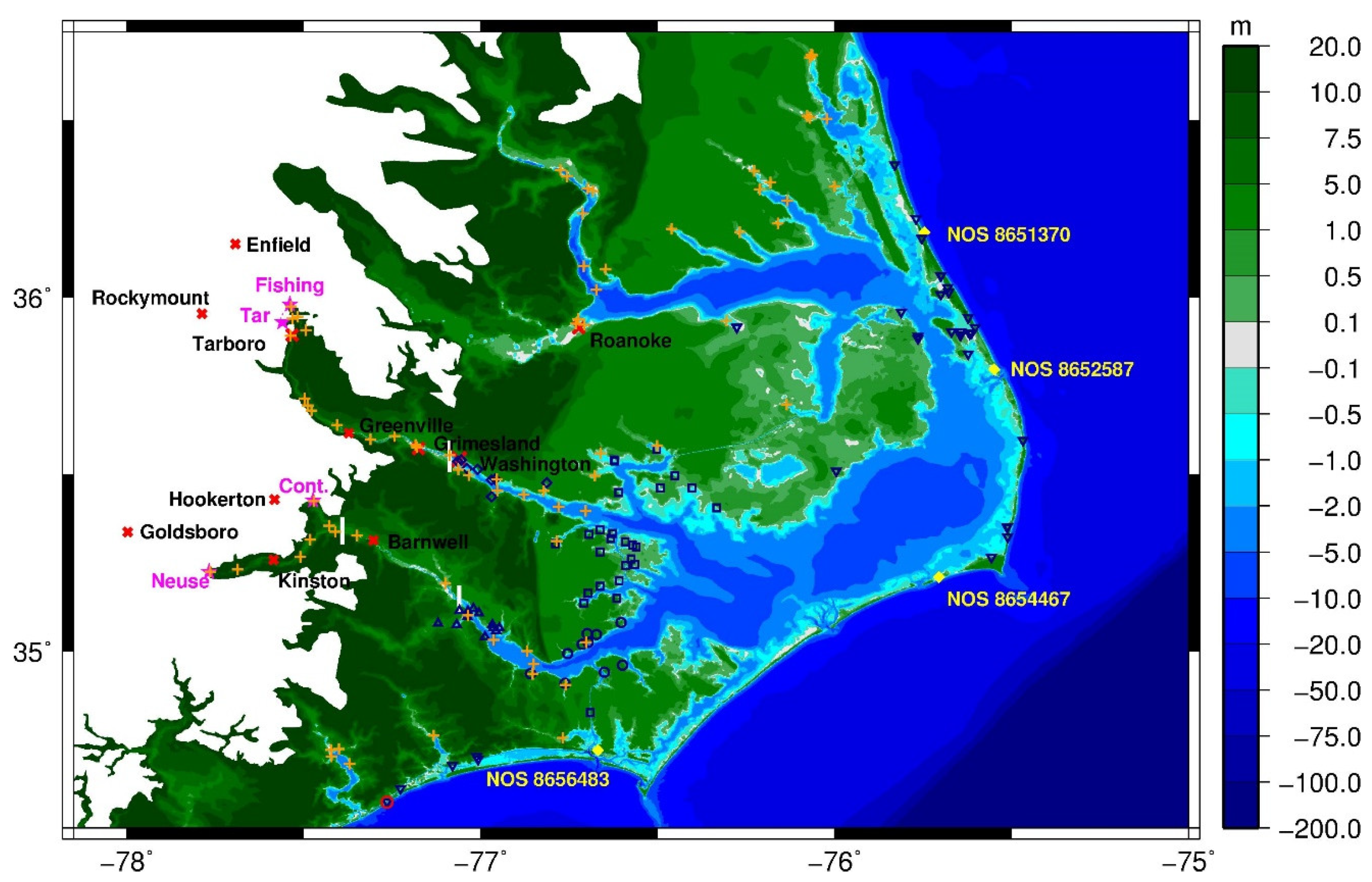
Now that mass balance and consistency have been established for the methodology, real-world case studies for Hurricane Irene are presented to determine the validity and accuracy of the new source terms. Irene made landfall near the area of Cape Lookout in North Carolina at 1200 UTC on 27 August 2011 and caused significant flooding along the east coast of the United States. Significant rainfall was measured during Hurricane Irene and the highest rainfall (around 40 cm) was recorded in the eastern portion of North Carolina around the study area of the Tar-Neuse-Pamlico sound. Hurricane Irene produced a storm surge along the Outer Banks of North Carolina of about 2.1 m near the Oregon Inlet Marina [42].

Hurricane Irene was chosen as the test storm for the following reasons: (1) it directly impacted the study region; (2) validated meteorological forcing information based on actual recorded data (i.e., OWI winds [43] and MRMS precipitation [34]) is readily available; (3) measurements for resulting water levels (for use in validation) are available from both NOAA and USGS sources [38,44]; (4) measurements of rainfall during the storm are available for verification of precipitation input; and (5) streamflows from the NWM reanalysis dataset [27] are available during this time period. Hurricane Florence in 2018 also affected the Pamlico Sound region with significant rainfall induced flooding and has many of these same data sources available; unfortunately, the reanalysis NWM version 1.2 dataset only covers January 1993 through December 2017 and streamflows for more recent events are not available.

4.1. Study Area

Previous work [23,45] has looked at connecting a hydrologic and hydrodynamic model in the North Carolina coast in the Tar-Neuse Pamlico areas. In particular, this work examined the behavior for the main stems of four different riverine areas in North Carolina: Tar and Neuse Rivers and Fishing and Contentnea Creeks but it did not include precipitation. The model for these studies was created with efficiency in mind and only has one element across each channel in the upland regions; on average, the mesh resolution of this domain varies from 50–100 m in upland channels, 750–1000 m on the floodplains, 100–500 m in channels and coastal marshes and 2–110 km in estuaries and the deep ocean. Furthermore, it was designed to more accurately match stage-discharge relationships under high streamflows, as the intent of the studies was to capture flood conditions rather than baseflow [14]. As a result, it is not expected that model results will match observations exactly. Figure 6 shows the bathymetry and topography of the model created for previous work in this study area; the connection points for the existing river flux methodology are the same for the current study and the locations of available NWM streamflows for the new methodology are also shown.

4.2. Sensitivity to Input Time Interval for Distributed Sources

The first set of tests examines sensitivity to the timing of the precipitation data that is input into ADCIRC as a distributed source. In order to incorporate the most accurate data, precipitation input fields are extracted from the MRMS data [34], which is synthesized from historical radar and field precipitation measurements. For these tests, only tides, winds and precipitation forcings are incorporated (no lateral source terms), in order to isolate the modeled water levels that are due solely to the addition of precipitation during the storm.

MRMS precipitation is available at different time frames depending upon the sources (reanalysis or real-time data), but typically data is available at either 2-min or 5-min increments. For these tests, it is assumed that frequent updating of the input precipitation would provide the most accurate representation of the actual rainfall since ADCIRC internally interpolates between input time snaps to define the precipitation field at each point in time throughout the simulation (e.g., precipitation may be input at hourly input intervals and the time step is on the order of seconds, such that the precipitation field is linearly interpolated through time between each hourly input for the thirty-six hundred time steps between, for a 1-second time step). A balance between lost accuracy and filesize must be made when determining the input frequency since a larger interval may completely miss rainfall peaks or conversely hold the precipitation rate higher for a longer duration than was recorded. These tests seek to determine what effects a larger temporal input interval for the rainfall will have on the final water levels. Intervals of 5, 15, 30 and 60 min are examined, with the finest 5-min interval used as the “true” solution (since this is the smallest time interval available during Hurricane Irene). This finest input model simulation is used as the “true” solution for comparative purposes only since the available validation data is limited in scope (when compared to the entire study region) and the purpose of these tests is to qualitatively judge the modeling results.

The simulation begins with a spinup period of only tidal forcing for 30 days (21 July–20 August 2011) then both winds (from OWI) and precipitation (from MRMS) are applied for the duration of the storm (20–30 August 2011). The rainfall amounts measured (over land) at NOAA stations during Hurricane Irene are provided in Figure 7a as a reference point [42,46], while Figure 7b,c show the accumulated rainfall obtained from the MRMS reanalysis at a 5-min interval (and processed as input in ADCIRC) and the actual applied rainfall for the study area. Recall that the precipitation in ADCIRC is only applied over the wet areas of the domain, such that most of the precipitation over land in Figure 7b has been “zeroed out” while some regions (that were affected by the storm surge) have non-zero precipitation (Figure 7c). Note that the precipitation input into ADCIRC (Figure 7b) occurred over the full ten-day storm simulation while the NOAA measurements (Figure 7a) were concentrated on the last six days of the event. However, since the storm did not make landfall in North Carolina until 27 August, both time frames capture the period of most intense rainfall. Despite the difference in accumulation time, note that the rainfall input into ADCIRC is similar in magnitude over the study area.

Turning now to the other time intervals, difference plots of applied rainfall and the resulting maximum water elevations are provided for each of the coarser time intervals (15-, 30- and 60-min) in Figure 8. Looking first at the precipitation differences in the left-hand column, it is noted that significant areas of both underestimation and overestimation, due to the large input time interval of 60-min, are seen for the total precipitation (first row). These underestimations and overestimations of the precipitation can also be seen for the next time interval of 30-min (middle row); however, they are less widespread and have smaller magnitudes (mostly within ±5 cm instead of ±10 cm). Meanwhile, there is a sharp decrease in these differences when a 15-min input interval is used for the precipitation rates (majority of colors fall in the ±2 cm range in bottom row). Turning now to the corresponding changes in simulated water surface elevations (right-hand column), it is noted that there is not a one-to-one correspondence between differences in applied rainfall and the final water surface elevations, particularly within the sound. For the 60-min interval, there is only a 1–2 cm difference within the body of the sound even though there are multiple regions with precipitation differences of 10 cm or more. Meanwhile, very little change is shown in the water surface elevations (WSEs) within the sound for the other two intervals, most likely because the precipitation is quickly distributed over the entire sound such that, on average, it does not change the WSE profile. However, some correlation can be drawn between the precipitation differences within the floodplain and riverine areas. Although not one-to-one in magnitude, most overestimations in precipitation within these regions cause higher final WSEs while significant underestimations in the precipitation result in WSE reductions; compare the regions outside of the black coastlines in the left and right panels for each time interval but note that the WSE differences are generally less than ±10 cm.

Given these results, it is suggested to input precipitation rates at 15-min intervals in order to accurately capture most of the precipitation during a tropical storm; however, intervals of 30 min also produce acceptable results if the user is willing to accept slightly higher deviations in the final WSE.

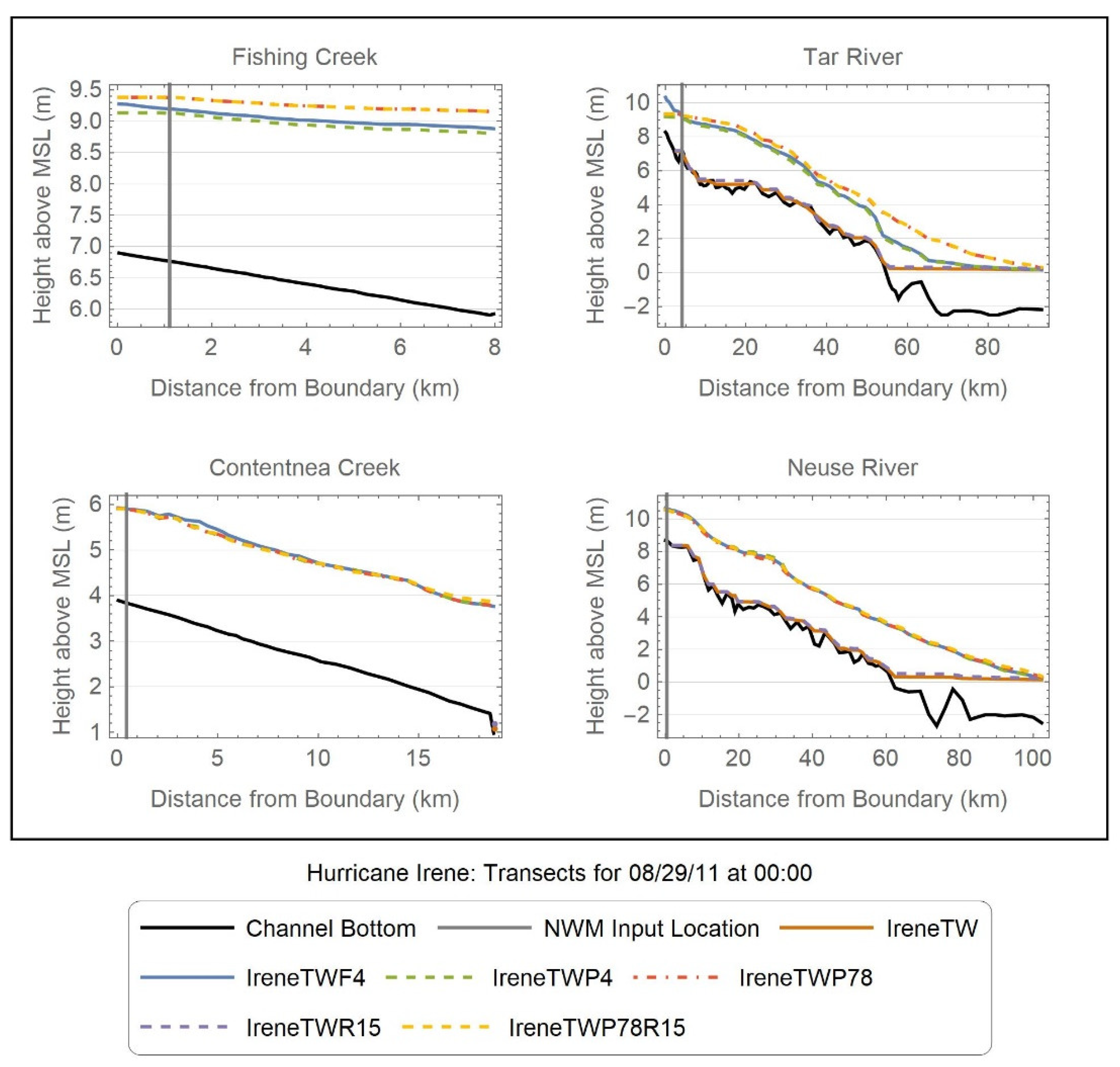
4.3. Validation of New Source Terms for Hurricane Irene

In this section, various simulations with and without the new source terms are evaluated against available data collected during and after Hurricane Irene. A summary of the simulation parameters, model descriptions and naming conventions used in the remaining figures and discussion is given in

Table 3. Summary of model setup and naming conventions for validation study.

Run Name	Description/Forcing	Spinup 21 July to 20 August 2011	Storm 20 August to 30 August 2011	Spindown 30 August to 9 September 2011
TW	Tides + Wind	T	TW	−
TWF4	Tides + Wind + Flux4	TF4	TWF4	TF4
TWP4	Tides + Wind + Point4	TP4	TWP4	TP4
TWP78	Tides + Wind + Point78	TP78	TWP78	TP78
TWR15	Tides + Wind + Rain15	T	TWR15	−
TWP78R15	Tides + Wind + Point78 + Rain15	TP78	TWP78R15	TP78

Notation for simulation acronyms: source terms included during each phase of the simulation (spinup, storm, spindown) can include Tides, Winds, boundary Fluxes, lateral/Point sources and Rainfall. The number after the different sources indicates either the number of sources or the time increment (in minutes) used. Spindown simulations are only included for the riverine input options.

.

During the event, timeseries of water heights and/or streamflows were recorded at seven USGS gauges [38]; additionally, water heights are available at four NOS stations [44] within the study area during this time frame. Various highwater marks (HWMs) were collected and analyzed for quality after the storm [47]. Of the one hundred HWMs available, ninety-two were categorized as Good or Excellent and are used herein; fifty-seven of these (in the immediate Tar/Neuse River basins) were further categorized by location within the study region. Most of the remaining HWMs are within the region of the domain that is affected by wind driven waves and are thus not expected to have good correlation since the additional influence of wave heights is not included in these simulations. Some of the floodplain and lower estuary locations are still influenced by waves, but improvement due to the additional source terms is still indicated. Locations of the available data sources were shown in Figure 6.

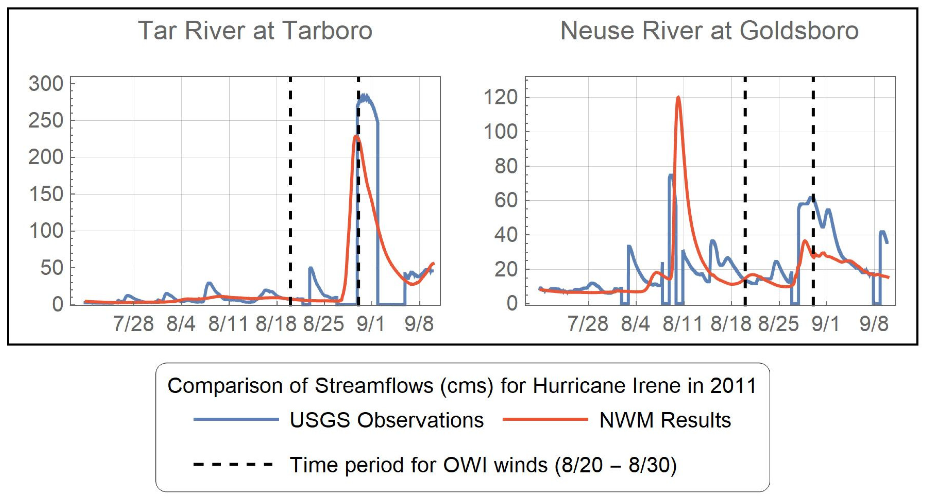
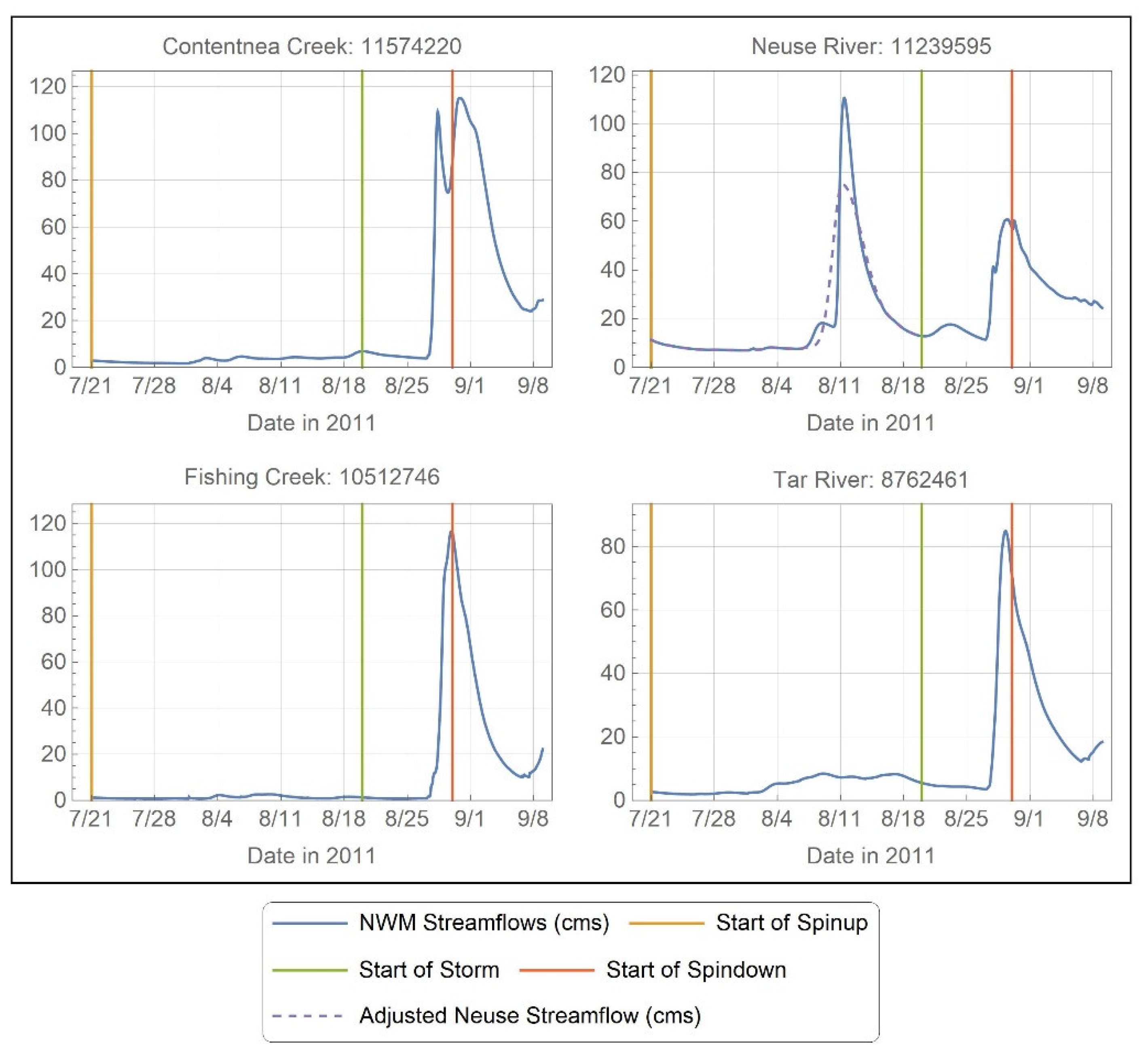
4.3.1. Streamflow Input

In order to properly assess the addition of streamflows to the ADCIRC hydrodynamic model, it is first necessary to get an idea of how accurate the NWM input streamflows are. Within the study region, there are four USGS gauges with recorded streamflow. There are four additional gauges located upstream of the NWM insertion points for all main features; however, only the gauges for the Neuse River (Goldsboro) and Contentnea Creek (Hookerton) were examined as the other two have significant flows added downstream of the USGS gauges relative to the connection points in the ADCIRC model; the relative location of these gauges and insertion points was shown in Figure 6. Plots of extracted NWM streamflows versus the observed USGS gauge streamflows for these six locations were examined in order to determine the relative accuracy of the NWM input being fed into ADCIRC; the two gauges closest to the Tar and Neuse insertion points are shown in Figure 9 while in Figure S1 all six are included. In general, the timing for peak flows is fairly accurate for both the Tar and Neuse Rivers; but the magnitude is underestimated by about 20% at Tarboro while the 10 August peak in the Neuse has 40% higher flows than were measured and the peak near 30 August is underestimated by 40–60% (depending upon the location in the river). This error in input accuracy will necessarily affect the comparison of the ADCIRC output at the USGS locations.

Actual NWM streamflows at the input points for the four main stems are shown in Figure 10 for the 21 July through 9 September 2011 timeframe. Unfortunately, the coarse mesh used in this study is unable to stably simulate the sharp streamflow increase in the Neuse near August 10 (each of the four main river reaches is represented by a single element across the channel and the meandering sections can become unstable during extremely high streamflows due to the wet/dry algorithm). However, further comparison of the extracted NWM streamflows and the observed USGS streamflows in the Neuse River indicate that this peak is exaggerated in the NWM results (Figure 9 and Supplementary). Therefore, a peak more comparable to the measured USGS values was constructed using piecewise normal distributions (dashed purple in Figure 10); this adjusted Neuse streamflow was used for all of the riverine input simulations).

Due to the hydrologic peak coming near the end of the storm, a modest “spindown” of riverine flows is typically required to capture all of the high streamflows; thus, the additional ten-day spindown was used for Hurricane Irene to ensure that all of the upland flow has had a chance to be routed to the coastal region.

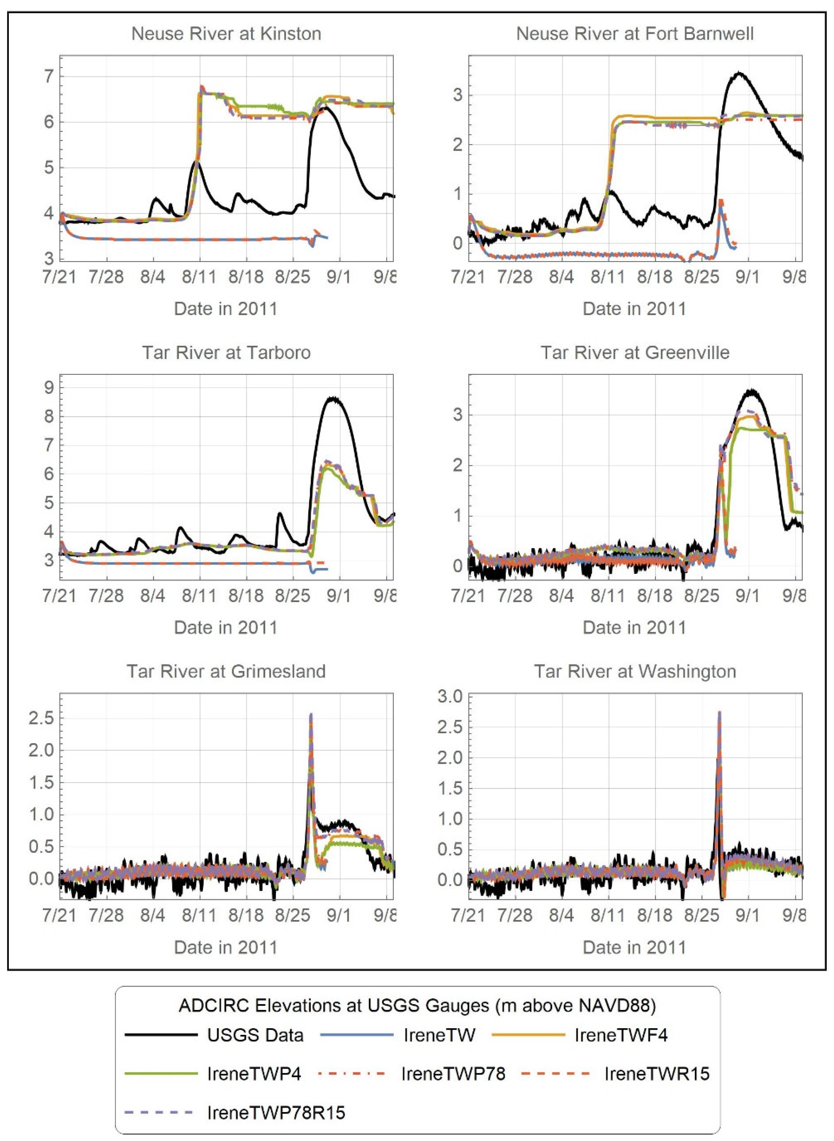
4.3.2. Comparison of Results with Old and New Methodologies

Transects are developed along the center of each of the main stems (Tar, Fishing, Neuse and Contentnea) for the simulations given in Table 3 and are used to compare model results during Hurricane Irene. For these transects, the channel bottom is represented by the bathymetry at the center of the channel, a distance of zero corresponds to the ADCIRC model boundary at the end of the river and the ending location of each transect was shown in Figure 6. Transects along these main reaches (near the end of the storm) and timeseries just below the NWM insertion point are provided in Figure 11 and Figure 12.

Since the model domain incorporates the rivers all the way to the ADCIRC model boundary for the four features shown in Figure 6, this allows for a direct comparison of the lateral inflow methodology to the standard river flux boundary condition. For the time shown in Figure 11, the two methods (TFW4 and TWP4) are fairly consistent; however, this changes with time, particularly near peaks and during the spinup phase (Figure 12), when a wet/dry instability occurs in Contentnea Creek for the TWF4 simulation near August 11. Closer examination of transects, at various times, reveals that the two riverine input methods are consistent (a sufficient distance away from the flux boundary) in all four riverine features except when one or the other simulation develops random wet/dry “ponding” near any of the features. Due to the nature of the built-in ADCIRC wet/dry procedure, these changes in wet/dry state are somewhat random (more on this when Figure 13 is discussed).

Water levels increase significantly in the Tar River and Fishing Creek with the additional lateral inflows from the upland surface runoff, but more minor changes are noted in the Neuse River and Contentnea Creek (TWP78 and TWP78R15 in Figure 11). There are only a few additional NWM features that are added along the length of the Neuse River and Contentnea Creek while several other tributaries join along the length of the Tar River and Fishing Creek. Most notably, Deep Creek joins near the confluence of Fishing and Tar and the addition of this larger reach causes additional water to backflow into Fishing Creek, which is already flooded due to its own elevated streamflow. Meanwhile, the inclusion of the downstream features along the Tar River cause 1–2 m of additional water depth as it approaches the coast. While the transect depths may only exhibit minor changes in the center of the channels, an examination of the flooding extents (not shown herein) reveals that the water levels in the rivers increase enough that many parts of the channels experience water spreading outside of the banks with the introduction of these additional streamflows; in particular both the Neuse and Tar Rivers have extensive flooding as they approach the coastal region (shown below in Figure 13).

It is important to recall that for the lateral inflow methodology, the streamflow values are not typically input directly at the model boundary, as is true for the flux boundary condition (e.g., the nearest ADCIRC node to the NWM feature is located nearly 5 km into the domain for the Tar River); thus, there is a deviation near the boundary for the lateral inflow water levels relative to the river flux levels. These deviations are due to the fact that there is no streamflow input until the solid gray vertical lines (Figure 11); above this location the water level is flat across the channel and behaves like a lake. However, it should be noted that the water levels for the different forcing mechanisms quickly approach the same values as you progress down the channels from the point source input location. These results further confirm that the lateral inflow (through the addition of a source term in the continuity equation) is consistent with the river flux boundary methodology (below the input location) and there is no need to evaluate a pure flux for riverine inputs away from the model domain boundary. However, it is still recommended that very large rivers (e.g., the Mississippi River in Louisiana) should be simulated with the river flux boundary since they are easily resolved with several larger elements and have consistently high streamflows. Additionally, any larger feature where accurate results are required above the point source input location should also be simulated using the river flux boundary.

While not immediately clear from the transects or timeseries, the river channels for both of the model runs without riverine input (TW and TWR15) dry out almost immediately and only rewet occasionally during the storm. For these two simulations, Fishing and Contentnea Creeks remain dry throughout the simulation (after drying) while the Tar and Neuse Rivers have some water in the low-lying areas. Note that the small vertical portion right at the beginning of the timeseries (spinup starts on 21 July) in Figure 12 represents the time it takes for the river to either dry out or adjust to the steady state WSE from the artificial value (the initial river elevation is equivalent to a WSE of 0.5 m above the channel bottom for this study) applied at the beginning of the spinup. Meanwhile, the timeseries along the Neuse River indicates that precipitation contributes a significant amount (0.3–0.4 m) of additional elevation at this location during the storm (from about 23 August to 28 August).

Finally, relative differences due to the new source terms are explored by computing differences in the maximum water surface elevations for various combinations of the simulations in Table 3; herein, three main differences are explored:

• Influence of precipitation: TWR15 less TW
• Influence of new riverine methodology: TWP4 less TWF4
• Influence of additional NWM sources available with the new methodology: TWP78 less TWF4

A qualitative comparison of the flooding extents and depths is explored for the Pamlico Sound region. Figure 13 shows the maximum WSE from the storm phase with both of the new source terms (IreneTWP78R15), as well as the above differences in WSEs. For all difference plots, negative values indicate regions where the base simulation (TW or TWF4) has higher water levels than the improvement being compared (TWR15, TWP4 or TWP78); conversely, positive values indicate regions where the improved model has higher water levels. Additionally, the darkest colors indicate a region where the wet/dry state has changed for the two models being compared (red if base model is dry and blue if improved model is dry). Note that for all cases, the contours indicate actual changes in WSE; so for regions that changed between wet/dry, the contour is the actual WSE of the wet model.

Looking first at the maximum water surface elevations with both of the new source terms activated (Figure 13a), note that the contours represent actual heights above MSL, not depths (the actual depths in the upper rivers are closer to 1–3 m). Although a difference plot is not shown for TWP78R15 less TW, adding both sources results in a larger region of the sound itself with higher water levels (spreading out towards the outer banks). Differences in WSEs due only to precipitation (Figure 13b), indicate that most of the sound and much of the surrounding floodplain has 0.1 m to 0.25 m higher water surface elevations due to the additional source term and scattered regions of the floodplain have up to 0.5 m to 1.0 m higher results. Meanwhile, both of the riverine difference plots (Figure 13c,d) exhibit similar behavior: focused changes within and near the rivers themselves and seemingly random changes to the floodplain closer to the coastline. As these random patches occur for both the riverine comparisons, they cannot be due to the addition of the 74 extra NWM streamflows (Figure 13c only has the four main streamflows added). Therefore, they must be due to random/small changes in how the wet/dry algorithm decides which elements have been wetted at each time step, since no other model parameters have changed and the four main riverine streamflows should not be influencing these regions (evidenced by the large swath of zero change between the upper rivers and the coastline). However, the small increase shown near −77.5 34.75 in Figure 13d is due to the addition of five NWM streamflows near that region. Focusing just on the rivers, Contentnea Creek overflows the banks and wets more of the floodplain for both NWM comparisons (Figure 13c,d), while much of the Tar River and Fishing Creek also floods under the additional streamflows added in the TWP78 simulation. However, the Neuse River remains largely unchanged and, in some areas, produces about 10 cm less WSE under the lateral methodology (as compared to the existing flux boundary methodology).

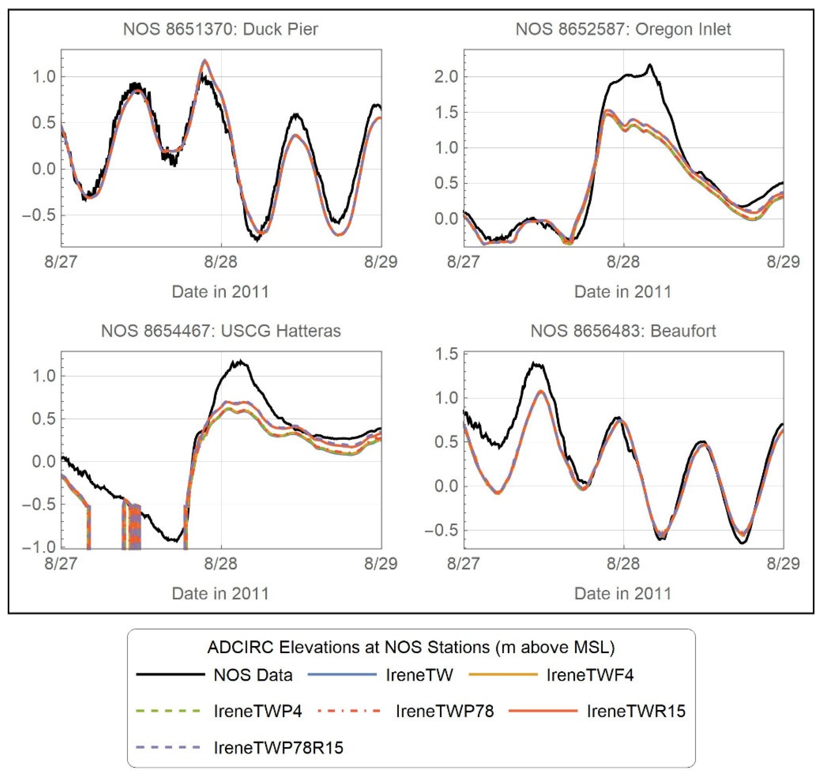
4.3.3. Validation of Model Results

Hydrographs at the available USGS stations (Figure 14) and tidal NOS stations (Figure 15) were created for the entire span of the model results. Where possible, the VDatum tool [48] was used to convert the ADCIRC results from a MSL datum to NAVD88 in order to compare to the USGS gauges. However, for the furthest inland areas no corrections are available as they are well outside the tidal zone. Instead, the modeled spinup timeseries (near base streamflow conditions) were compared to the observed USGS gauge heights and corrections were estimated from the differences. These estimated corrections were then applied to all modeled results (spinup, storm and spindown) at these USGS locations in order to facilitate a reasonable comparison of modeled and observed quantities.

As was found in previous studies [14,49], the modeled water elevations in the Neuse River are not as indicative of the measured USGS observations. Particularly, the pre-storm peak near 11 August is overestimated while the storm peak near 30 August is underestimated (at Fort Barnwell); however, recall that the NWM input streamflows were not as accurate in the Neuse River. Furthermore, the receding limbs of the modeled results do not subside as quickly in the Neuse River as was observed at the USGS gauges (for either of the riverine input methods). This behavior has been noted by Tromble and Bush in previous studies and is most likely related to the coarse grid resolution within the rivers themselves, as well as the model design preferentially matching peak streamflows for better flood prediction thus resulting in improper stage-discharge relationships at lower flow conditions [14,49]. Had the water levels subsided after the 11 August peak, then the storm peak at the Kinston station would likely have been underestimated as well. Despite these challenges, the addition of streamflow manages to capture the peak stage relatively well at most locations and is certainly a better representation of observed stages than the simulations (TW and TWR15) that do not include the streamflow and are thus unable to capture the additional water elevations after 30 August (at all stations). Meanwhile, the addition of precipitation provides a better match to observations at the lower stations (Greenville, Grimesland and Washington) but does not have a significant impact in the upper reaches unless the lateral sources are also included (TWR15 nearly identical to TW at Kinston, Fort Barnwell and Tarboro).

For the coastal observation at the NOS stations (Figure 15), first recall that waves are not included in these simulations, so it is not expected that model results will match perfectly with the data. Additionally, note that the model is not finely resolved along the coast as the intention in the original study was a balance between efficient computation and sufficient accuracy (thus the location for the Hatteras station does not refine the small channels in the shipyard and the model results actually dry out for some times). The takeaway from these plots is that the results with precipitation (TWR15 and TWP78R15) have higher accuracy than those without at these coastal regions (as much as 20 cm difference), since the additional water added by the lateral inflows is not expected to impact the coastal region as much as the riverine areas.

Scatterplots of the modeled maximum water surface elevations versus the measured HWMs were created for all of the simulations listed in Table 3 and are shown in Figure 16. The majority of the HWM locations are not located in the most inland portion of the Tar and Neuse drainage basins; therefore, very little difference is noted between the base TW results and the various riverine input methods (TWF4, TWP4 and TWP78) and only the TWP78 HWM results are shown herein (yellow/red and blue/cyan best-fit lines and HWM data points generally overlie one another). The most significant improvement in the HWMs due to the new source terms occurs with the addition of precipitation (slope and R² values are both closer to the ideal value of 1). The single “Other” location that shows a significant improvement due to the addition of lateral inflows (measured HWM around 3.2 m), is indicated by the red circle in Figure 6. Note that there are five NWM insertion points near this HWM that are neglected in the current methodology; their location indicates that the addition of NWM sources near the coast can have a more direct impact on coastal flooding than the inland/upstream sources.

A summary of the best-fit statistics by location category is given in

Table 4. Comparison of linear best-fit statistics of HWM scatter plots by location category.

Simulation	Best-Fit Statistics	Neuse River Lower	Neuse River Upper	Tar River	Tar/Neuse Floodplains	Other	57 Tar/Neuse Region	All 92 Available
TW	Slope	0.689	0.944	1.125	0.801	0.645	0.852	0.792
	R2	0.988	0.996	0.988	0.984	0.955	0.962	0.947
TWF4	Slope	0.696	0.960	1.130	0.806	0.681	0.860	0.808
	R2	0.988	0.996	0.987	0.984	0.971	0.962	0.954
TWP4	Slope	0.695	0.958	1.129	0.806	0.671	0.859	0.804
	R2	0.988	0.996	0.987	0.984	0.971	0.962	0.953
TWP78	Slope	0.696	0.959	1.132	0.806	0.675	0.860	0.806
	R2	0.988	0.996	0.987	0.984	0.972	0.962	0.954
TWR15	Slope	0.722	0.985	1.172	0.860	0.713	0.898	0.846
	R2	0.988	0.994	0.986	0.983	0.972	0.963	0.955
TWP78R15	Slope	0.729	1.008	1.177	0.866	0.713	0.906	0.852
	R2	0.988	0.992	0.986	0.983	0.974	0.962	0.955

(Figure S2 shows the HWM scatterplot with best-fit lines categorized by location for TWP78R15; all other simulations have similar behavior). Statistically, there is very little improvement noted for any of the riverine input options due to the lack of HWMs near the banks of the rivers themselves, while the addition of precipitation most improves the slope and R² values. The Lower Neuse, Floodplain and Other locations are missing some modeled height due to wave impacts, so the linear correlation is not as high at these locations. Finally, all simulations (including the base, TW) overestimate the water surface elevations in the Upper Tar, indicating that there is likely a bathymetry or resolution issue in that region of the model domain.

This is not a true “total water level” simulation, as waves were not included; however, as the focus of this study is to provide general proof of concept and validation of the methodology rather than a true hindcast validation of the near-shore coastal response, the lack of wave physics will not alter the results significantly. Previous studies have shown that waves are more influential in the near-shore tidal zone and do not often travel upriver much beyond the tidal limit except in cases of extreme storm surge [23,45]. Therefore, the lack of waves will mostly affect the comparisons at the NOS stations but should have little to no bearing on the inland USGS results.

5. Conclusions

A new methodology for adding distributed and point sources to the ADCIRC hydrodynamic model has been presented (Section 2). The methodology was verified with ideal test cases for each source type and shown to be consistent (Section 3). The methodology was applied to Hurricane Irene along the North Carolina coast and validated with available data (Section 4); however, since waves were not included, this is not a full validation of the storm hindcast but rather of the new methodology. Several takeaways can be summarized:

• The new methodology provides a way to incorporate riverine input in regions of an ADCIRC mesh without fully refining the model domain all the way to the model boundary, as was previously required in the river flux boundary condition methodology. The new methodology is consistent with the previous methodology; however, it is recommended that large rivers (particularly those that are near the coastal region, e.g., Mississippi River) should continue to be input into ADCIRC using the river flux methodology, as it distributes the streamflow across the entire river instead of inputting at a single point. Additionally, any larger feature where accurate results are required above the point source input location should also be simulated using the river flux boundary.
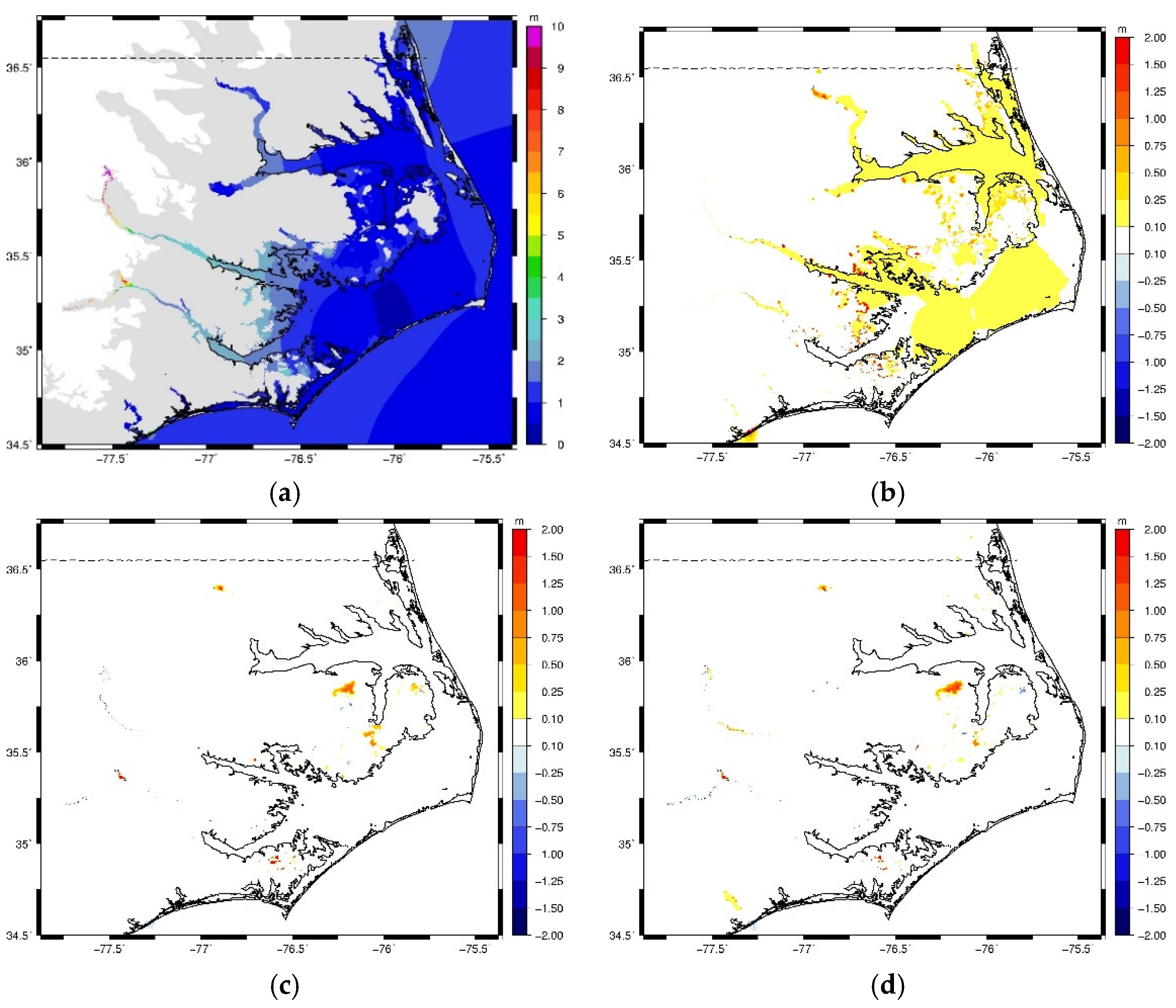
• The addition of riverine streamflow through lateral inflows can substantially impact both upland regions and the coastal transition zone, particularly if the peak riverine flows coincide with the storm surge. However, timing is specific to each storm and coastal impacts are also dependent upon the timing and magnitude of the streamflows. Although there was little coastal impact due to the riverine sources during Hurricane Irene, there was substantial flooding near the main Tar River reach (1–2 m), which would not be captured without the additional 74 NWM sources. The collection of more HWMs near major riverine reaches (after extreme weather events) would be helpful for further validating the methodology; although riverine flooding is noted in Figure 13d, no change is noted in the HWM analysis for the TWP4 and TWP78 simulations since most of the HWMs are not located in the immediate riverine area.
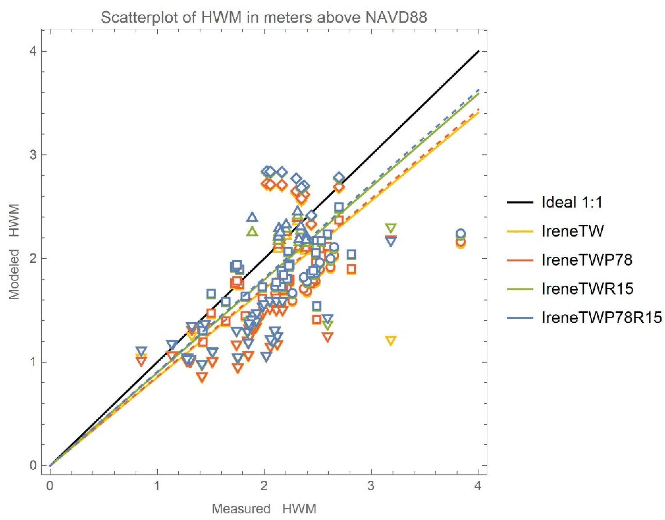
• The addition of precipitation over the wet ADCIRC nodes impacted a larger area, with a 10–20 cm increase in maximum water surface elevations throughout Pamlico Sound and the wet riverine reaches (Figure 13b) and higher localized impacts where temporal changes of 30–50 cm were noted in the Neuse River (Figure 12). The distributed source is more readily spread out over the water nodes but does not begin to accumulate over upland regions until they have already wetted due to riverine flooding or storm surge. HWM analysis indicates that the addition of precipitation provides the most improvement in the best-fit slope: 0.846 for TWR15 and 0.852 for TWP78R15, as compared to 0.808 for the current state of the model (TWF4).
• Due to the amount of data required, it is recommended that precipitation be input at intervals of 15 or 30 min to maximize accuracy in rainfall input and minimize data processing.

Additionally, there are several areas of future work that remain as the connection of hydrologic and hydrodynamic models is still in its infancy. These include:

• More efficient and frequent data entry (for both distributed and point sources) utilizing the ADCIRC coupling cap within the NOAA Environmental Modeling System framework [50] instead of file IO.
• One of the greatest needs is more accurate bathymetry in the upland rivers. While several databases exist for coastal bathymetry, much of the inland hydrology data is collected for individual studies and is not as readily (or publicly) available. Nor is it in a format that is readily applied to hydrodynamic models, since they are not as finely resolved as the riverine cross-sections created for typical hydrologic models (e.g., HEC-RAS [51]). A method for finding accurate and representative “average” cross-sectional bathymetries for the rivers must be developed.
• Additional studies with other storms may provide more information about conditions when the existing flux boundary riverine input is more accurate than using the lateral source term. No hard and fast rules can be developed from a single study and further guidance would be useful for modelers.
• Finally, the coupling with the NWM thus far is static in location and efforts are ongoing to create a dynamic coupling, whereby the upstream connection point will move as the floodplain wets (due to surge or riverine flooding). This will allow for more accurate upland flooding as the source will more accurately reflect the actual location of the incoming streamflow. A careful balance must be maintained when the input location is chosen since the ADCIRC hydrodynamic model is not made to be a hydrologic routing model and will not be as accurate as the hydrologic model itself in the furthest upland regions. However, this dynamic coupling in conjunction with further improvements to the wet/dry module within ADCIRC will improve the overall accuracy for the upland riverine flooding.

References

1. Blake, E.S.; Zelinsky, D.A. National Hurricane Center Tropical Cyclone Report: Hurricane Harvey (AL092017); NOAA Technical Report; National Oceanic and Atmospheric Administration, National Hurricane Center: Miami, FL, USA, 2018; p. 77.
2. Cangialosi, J.P.; Latto, A.S.; Berg, R. National Hurricane Center Tropical Cyclone Report: Hurricane Irma (AL112017); NOAA Technical Report; National Oceanic and Atmospheric Administration, National Hurricane Center: Miami, FL, USA, 2021; p. 111.
3. Stewart, S.R.; Berg, R. National Hurricane Center Tropical Cyclone Report: Hurricane Florence (AL062018); NOAA Technical Report; National Oceanic and Atmospheric Administration, National Hurricane Center: Miami, FL, USA, 2019; p. 98.
4. Wahl, T.; Jain, S.; Bender, J.; Meyers, S.D.; Luther, M.E. Increasing risk of compound flooding from storm surge and rainfall for major US cities. Nat. Clim. Chang. 2015, 5, 1093–1097. [Google Scholar] [CrossRef]
5. Stewart, S.R. National Hurricane Center Tropical Cyclone Report: Hurricane Matthew (AL142016); NOAA Technical Report; National Oceanic and Atmospheric Administration, National Hurricane Center: Miami, FL, USA, 2017; p. 96.
6. Van Cooten, S.; Kelleher, K.E.; Howard, K.; Zhang, J.; Gourley, J.J.; Kain, J.S.; Nemunaitis-Monroe, K.; Flamig, Z.; Moser, H.; Arthur, A.; et al. The CI-FLOW Project: A System for Total Water Level Prediction from the Summit to the Sea. Bull. Am. Meteorol. Soc. 2011, 92, 1427–1442. [Google Scholar] [CrossRef] [Green Version]
7. Dresback, K.M.; Fleming, J.G.; Blanton, B.O.; Kaiser, C.; Gourley, J.J.; Tromble, E.M.; Luettich, R.A.; Kolar, R.L.; Hong, Y.; Van Cooten, S.; et al. Skill assessment of a real-time forecast system utilizing a coupled hydrologic and coastal hydrodynamic model during Hurricane Irene (2011). Cont. Shelf Res. 2013, 71, 78–94. [Google Scholar] [CrossRef]
8. Taylor, A.; Huiquig, L. Latest Development in NWS’ Sea Lake and Overland Surges From Hurricanes Model. In Proceedings of the 18th Symposium on the Coastal Environment, American Meteorological Society Annual Meeting; Boston, MA, USA, 1 April 2020, p. 10. Available online: http://ams.confex.com/ams/2020Annual/mediafile/Manuscript/Paper370583/SLOSH_MPI_AMS-2020.pdf. (accessed on 15 October 2022).
9. NOAA Water Initiative. Available online: https://www.noaa.gov/water/explainers/noaa-water-initiative-vision-and-five-year-plan (accessed on 1 May 2020).
10. Zscheischler, J.; Westra, S.; van den Hurk, B.J.J.M.; Seneviratne, S.I.; Ward, P.J.; Pitman, A.; AghaKouchak, A.; Bresch, D.N.; Leonard, M.; Wahl, T.; et al. Future Climate Risk from Compound Events. Nat. Clim. Change 2018, 8, 469–477. [Google Scholar] [CrossRef]
11. Flowerdew, J.; Horsburgh, K.; Wilson, C.; Mylne, K. Development and evaluation of an ensemble forecasting system for coastal storm surges. Q.J.R. Meteorol. Soc. 2010, 136, 1444–1456. [Google Scholar] [CrossRef] [Green Version]
12. Beardsley, R.C.; Chen, C.; Xu, Q. Coastal Flooding in Scituate (MA): A FVCOM Study of the 27 December 2010 Nor’easter. J. Geophys. Res. Ocean. 2013, 188, 6030–6045. [Google Scholar] [CrossRef] [Green Version]
13. Bowler, N.E.; Arribas, A.; Mylne, K.R.; Robertson, K.B.; Beare, S.E. The MOGREPS short-range ensemble prediction system. Q. J. R. Meteorol. Soc. 2008, 134, 703–722. [Google Scholar] [CrossRef]
14. Tromble, E.M.; Kolar, R.L.; Dresback, K.M.; Hong, Y.; Vieux, B.; Luettich, R.A.; Gourley, J.J.; Kelleher, K.E.; Van Cooten, S. Aspects of Coupled Hydrologic-Hydrodynamic Modeling for Coastal Flood Inundation. In Proceedings of the 11th International Conference on Estuarine and Coastal Modeling, Reston, VA, USA, 4–6 November 2009; Spaulding, M.L., Ed.; ASCE: Seattle, WA, USA; pp. 724–743. [Google Scholar]
15. Ray, T.; Stepinski, E.; Sebastian, A.; Bedient, P.B. Dynamic Modeling of Storm Surge and Inland Flooding in a Texas Coastal Floodplain. J. Hydraul. Eng. 2011, 137, 1103–1110. [Google Scholar] [CrossRef]
16. Torres, J.M.; Bass, B.; Irza, N.; Fang, Z.; Proft, J.; Dawson, C.; Kiani, M.; Bedient, P. Characterizing the hydraulic interactions of hurricane storm surge and rainfall–runoff for the Houston–Galveston region. Coast. Eng. 2015, 106, 7–19. [Google Scholar] [CrossRef] [Green Version]
17. Ye, F.; Zhang, Y.J.; Yu, H.; Sun, W.; Moghimi, S.; Myers, E.; Nunez, K.; Zhang, R.; Wang, H.V.; Roland, A.; et al. Simulating Storm Surge and Compound Flooding Events with a Creek-to-Ocean Model: Importance of Baroclinic Effects. Ocean. Model. 2020, 145, 101526. [Google Scholar] [CrossRef]
18. Zhang, Y.; Ye, F.; Yu, H.; Sun, W.; Moghimi, S.; Myers, E.; Nunez, K.; Zhang, R.; Wang, H.V.; Roland, A.; et al. Simulating Compound Flooding Events in a Hurricane. Ocean. Dyn. 2020, 70, 621–640. [Google Scholar] [CrossRef]
19. Schiller, R.V.; Kouraftalou, V.H. Modeling River Plume Dynamics with the Hybrid Coordinate Ocean Model. Ocean. Model. 2010, 33, 101–117. [Google Scholar] [CrossRef]
20. Ye, F.; Huang, W.; Zhang, Y.; Moghimi, S.; Myers, E.; Pe’eri, S.; Yu, H. A Cross-Scale Study for Compound Flooding Processes During Hurricane Florence. Nat. Hazards Earth Syst. Sci. 2021, 21, 1703–1719. [Google Scholar] [CrossRef]
21. Brown, C.; Kovalenko, S.; Akan, C.; Tripathee, B.; Resio, D. Preliminary Design and Development of a Coupled Water Resources Resiliency Model of the St. Johns River Watershed Florida, USA. Proceedings 2020, 48, 19. [Google Scholar]
22. Leuttich, R.A.; Westerink, J.J. Formulation and Numerical Implementation of the 2D/3D ADCIRC Finite Element Model Version 44. Available online: https://adcirc.org/wp-content/uploads/sites/2255/2013/07/adcirc_theory_2004_12_08.pdf (accessed on 8 May 2022).
23. Dresback, K.; Szpilka, C.; Xue, X.; Vergara, H.; Wang, N.; Kolar, R.; Xu, J.; Geoghegan, K. Steps Towards Modeling Community Resilience Under Climate Change: Hazard Model Development. J. Mar. Sci. Eng. 2019, 7, 225. [Google Scholar] [CrossRef] [Green Version]
24. Courant, R.; Friedrichs, K.; Lewy, H. On the Partial Difference Equations of Mathematical Physics. IBM J. Res. Dev. 1967, 11, 215–234. [Google Scholar] [CrossRef]
25. Bilskie, M.V. (University of Georgia, Athens, Georgia USA). 2D Rainfall-Runoff Module for ADCIRC; presented to the ADCIRC Coordination monthly webinar on 26 June 2022.
26. Gochis, D.J.; Barlage, M.; Dugger, A.; FitzGerald, K.; Karsten, L.; McAllister, M.; McCreight, J.; Mills, J.; RefieeiNasab, A.; Read, L.; et al. The WRF-Hydro Modeling System Technical Description, Version 5.0; NCAR Technical Note; National Center for Atmospheric Research: Boulder, CO, USA, 2018; p. 107. [Google Scholar] [CrossRef]
27. NOAA National Water Model Reanalysis Model Data on AWS. Available online: https://docs.opendata.aws/nwm-archive/readme.html (accessed on 15 February 2021).
28. Kinnmark, I. The Shallow Water Wave Equations: Formulation, Analysis and Application. Lect. Notes Eng. 1986, 15, 1–87. [Google Scholar]
29. Lynch, D.R.; Gray, W.G. A Wave Equation Model for Finite Element Tidal Computations. Comput. Fluids 1979, 7, 207–228. [Google Scholar] [CrossRef]
30. Kolar, R.L.; Westerink, J.J.; Cantekin, M.E.; Blain, C.A. Aspects of Nonlinear Simulation using Shallow Water Models Based on the Wave Continuity Equation. Comput. Fluids 1994, 23, 523–538. [Google Scholar] [CrossRef]
31. Taylor, C.; Davis, J.M. Tidal and Long-Wave Propagation: A Finite Element Approach. Comput. Fluids 1975, 3, 125–148. [Google Scholar] [CrossRef]
32. Marchok, T.; Rogers, R.; Tuleya, R. Validation schemes for tropical cyclone quantitative precipitation forecasts: Evaluation of operational models for U.S. landfalling cases. Weather. Forecast. 2007, 22, 726–746. [Google Scholar] [CrossRef]
33. Zhang, J.; Qi, Y.; Langston, C.; Kaney, B.; Howard, K. A real-time algorithm for merging radar QPEs with rain gauge observations and orographic precipitation climatology. J. Hydrometeor 2014, 15, 1794–1809. [Google Scholar] [CrossRef] [Green Version]
34. Zhang, J.; Gourley, J. Multi-Radar Multi-Sensor Precipitation Reanalysis, Version 1.0; Open Commons Consortium Environmental Data Commons. 2018. Available online: https://edc.occ-data.org/nexrad/mosaic/ (accessed on 15 April 2021).
35. Flamig, Z.; Vergara, H.; Gourley, J. The Ensemble Framework For Flash Flood Forecasting (EF5) v1.2: Description and Case Study, Geosci. Model Dev. 2020, 13, 4943–4958. [Google Scholar] [CrossRef]
36. Geoghegan, K.M.; Fitzpatrick, P.; Kolar, R.L.; Dresback, K.M. Evaluation of a Synthetic Rainfall Model, P-CLIPER, for Use in Coastal Flood Modeling. Nat. Hazards 2018, 92, 699–726. [Google Scholar] [CrossRef]
37. U.S. Army Corps of Engineers; Hydrologic Engineering Center. HEC-HMS Hydrologic Modeling System, Technical Reference Manual CPD-74B; Hydrologic Engineering Center: Davis, CA, USA, 2000.
38. USGS Current Water Data for the Nation. Available online: https://waterdata.usgs.gov/nwis/rt (accessed on 20 April 2022).
39. Szpilka, C.M.; Dresback, K.M.; Kolar, R.L.; Moghimi, S.; Myers, E.P. Development of Accumulation Term in ADCIRC Hydrodynamic Model for Inclusion of Precipitation and Inland Hydrology; NOAA Technical Memorandum NOS CS 53; National Oceanic and Atmospheric Administration, National Ocean Service: Silver Spring, MD, USA, 2022; in press.
40. Dietrich, J.; Tanaka, S.; Westerink, J.; Dawson, C.; Luettich, R.; Zijlema, M.; Holthuijsen, L.; Smith, J.; Westerink, L.; Westerink, H. Performance of the Unstructured-Mesh, SWAN+ADCIRC Model in Computing Hurricane Waves and Surge. J. Sci. Comput. 2012, 52, 468–497. [Google Scholar] [CrossRef]
41. Pringle, W.J.; Wiraset, D.; Roberts, K.J.; Westerink, J.J. Global Storm Tide Modeling with ADCIRC v55: Unstructured Mesh Design and Performance. Geosci. Model Dev. 2021, 14, 1125–1145. [Google Scholar] [CrossRef]
42. Avila, L.A.; Cangialosi, J. National Hurricane Center Tropical Cyclone Report: Hurricane Irene (AL092011). NOAA Technical Report; National Oceanic and Atmospheric Administration, National Hurricane Center: Miami, FL, USA, 2011; p. 45. [Google Scholar]
43. Powell, M.; Houston, S.; Amat, L.; Morisseau-Leroy, N. The HRD Real-Time Hurricane Wind Analysis System. J. Wind. Eng. Ind. Aerodyn. 1998, 77, 58–64. [Google Scholar] [CrossRef]
44. NOAA Tides and Currents. Available online: http://tidesandcurrents.noaa.gov/ (accessed on 20 April 2022).
45. Yang, K.; Davidson, R.; Vergara, H.; Kolar, R.L.; Dresback, K.M.; Colle, B.A.; Blanton, B.O.; Wachtendorf, T.; Trivedi, J.; Nozick, L.K. Incorporating Inland Flooding into Hurricane Evacuation Decision Support Modeling. Nat. Hazards 2019, 96, 857–878. [Google Scholar] [CrossRef]
46. NOAA Tropical Cyclone Rainfall Data. Available online: https://www.wpc.ncep.noaa.gov/tropical/rain/tcrainfall.html (accessed on 10 April 2021).
47. USGS Flood Event Viewer. Available online: https://stn.wim.usgs.gov/FEV/#2011Irene (accessed on 20 April 2022).
48. NOAA/NOS’s VDatum 4.2.2: Vertical Datums Transformation. Available online: https://vdatum.noaa.gov/welcome.html (accessed on 1 May 2022).
49. Bush, S.T.; Dresback, K.M.; Szpilka, C.M.; Kolar, R.L. Use of 1D Unsteady HEC-RAS in a Coupled System for Compound Flood Modeling: North Carolina Case Study. J. Mar. Sci. Eng. 2022, 10, 306. [Google Scholar] [CrossRef]
50. Moghimi, S.; Vinogradov, S.; Myers, E.; Funakoshi, Y.; Van der Westhuysen, A.; Abdolali, A.; Ma, Z.; Liu, F. Development of a Flexible Coupling Interface for ADCIRC Model for Coastal Inundation Studies; NOAA Technical Memorandum NOS CS 41; National Oceanic and Atmospheric Administration, National Ocean Service: Silver Spring, MD, USA, 2019; p. 41.
51. Bruner, G.W. HEC-RAS, River Analysis System Hydraulic Reference Manual. Available online: https://www.hec.usace.army.mil/software/hec-ras/documentation/HEC-RAS_4.1_Reference_Manual.pdf (accessed on 30 April 2022).
Figure 1. Example of determining the lateral inflows or point sources given the location in longitude or latitude. The black dot represents the given location of the lateral inflow with the shaded triangles indicating the wetted elemental area used in determining the intensity. The red dot indicates the nodal location where this information is included within ADCIRC.
Jmse 11 00248 g001
Figure 2. (a) Temporal variation of precipitation intensities over a one-day simulation (value indicated in figure applied over the entire spatial domain), (b) Spatial variation of precipitation intensities (distribution applied for entire length of simulation for spatially varying test case and scaled by factor of zero to one for the spatial and temporally varying test case).
Jmse 11 00248 g002
Figure 3. (a) Idealized channel domain with node numbers for time series output indicated within the domain. Depths (below MSL) are shown in blue with the light gray area of the domain showing the land with topography above MSL. (b) Idealized streamflows used to test the lateral inflows.
Jmse 11 00248 g003
Figure 4. Model results compared to the steady state water depths with constant lateral inflows and river flux boundaries and with variable lateral inflows and river flux boundaries. Note that a distance of zero corresponds to the top of the channel at node 861.
Jmse 11 00248 g004
Figure 5. Elevation and velocity channel profiles at time t = 12 h and timeseries at the ideal test case input locations (top and middle of the channel) for the three different forcing mechanisms: river flux boundary condition, lateral inflow at the top of the channel and lateral inflow from the side (at the middle of the channel domain).
Jmse 11 00248 g005
Figure 6. Bathymetry and topography for the Tar-Neuse-Pamlico study area within North Carolina. Existing connection points for the river flux methodology are shown with magenta stars while the new NWM connection points are shown with orange plus signs. White bars indicate the end of the transects down the main stems (used for model comparison), which begin at the magenta stars. Data available for validation includes: USGS gaging stations (red X, names in black), tidal NOS stations (filled yellow diamonds), and high-water marks categorized by location (navy: squares—Tar/Neuse floodplains, circles—Lower Neuse, triangles—Upper Neuse, diamonds—Upper Tar and inverted triangles—Other). Red circle indicates location of Other HWM that is significantly impacted by the addition of the NWM streamflows.
Jmse 11 00248 g006
Figure 7. Accumulated rainfall (in cm) during Hurricane Irene obtained from: (a) NOAA [46] during 24–30 August 2011; (b) MRMS reanalysis data input into the ADCIRC model (at 5-min intervals) during 20–30 August 2011 and (c) actual rainfall amounts that were applied to wet nodes within the ADCIRC model. Solid black lines denote the coastline, but not the full water-only model domain.
Jmse 11 00248 g007
Figure 8. Difference plots of the applied precipitation (left-hand column) and resulting water elevations (right-hand column) during Hurricane Irene: (a) 60-min precipitation interval vs. 5-min precipitation interval, (b) 30-min precipitation interval vs. 5-min precipitation interval, (c) 15-min precipitation interval vs. 5-min precipitation interval. Note that all of the figures have the same scale, which does not have constant increments, and differences less than 1 cm are not shown.
Jmse 11 00248 g008aJmse 11 00248 g008b
Figure 9. Comparison of observed streamflows at USGS gauging stations to simulated streamflows at the nearest available NWM location.
Jmse 11 00248 g009
Figure 10. National Water Model input streamflows (cms) for the four main features in the study region during the simulation timeframe: Contentnea Creek, Neuse River, Fishing Creek and Tar River. The numbers following the names correspond with the NWM v1.2 feature identifications.
Jmse 11 00248 g010
Figure 11. Water level results from Hurricane Irene on 29 August 2011 for the four main stems in the Neuse-Tar-Pamlico area of North Carolina under the six simulation conditions give in Table 3. Black lines represent the channel bottom and solid gray vertical lines indicate the locations where the lateral inflow is input into ADCIRC from the NWM.
Jmse 11 00248 g011
Figure 12. Hydrographs (water surface elevation in meters above MSL) located just below the NWM insertion points on each of the four main rivers for the simulations given in Table 3.
Jmse 11 00248 g012
Figure 13. (a) Maximum WSE (above MSL) for the full TWP78R15 simulation with all source terms activated. Differences in maximum WSEs exploring influence of (b) precipitation addition (TWR15 less TW), (c) new lateral source term for riverine inputs (TWP4 less TWF4), and (d) additional riverine inputs (TWP78 less TWF4).
Jmse 11 00248 g013
Figure 14. Comparison of modeled water heights for all additional input source combinations relative to observations at select USGS gauge sites. Note that datum corrections for upland stations are approximate due to lack of tidal data that far upriver in the VDatum transformation tool.
Jmse 11 00248 g014
Figure 15. Comparison of modeled water heights for all additional input source combinations relative to observations at the available NOS stations (focused on timing of peak surge).
Jmse 11 00248 g015
Figure 16. Comparison of HWM scatter plots with new source terms. Shapes correspond to the locations shown in Figure 6 (diamonds—Tar River, triangles—Upper Neuse River, squares—Tar/Neuse floodplains, circles—Lower Neuse River, inverted triangles—all Other locations). Simulation abbreviations as per Table 3.
Jmse 11 00248 g016