Article

Spatial–Temporal Variations in Regional Sea Level Change in the South China Sea over the Altimeter Era

1
Center for Space Research and Technology, Huzhou Institute of Zhejiang University, Huzhou 313000, China
2
School of Ocean and Earth Science, Tongji University, Shanghai 200092, China
3
School of Software, Nanchang Hangkong University, Nanchang 330063, China
*
Author to whom correspondence should be addressed.
J. Mar. Sci. Eng. 2023, 11(12), 2360; https://doi.org/10.3390/jmse11122360
Submission received: 7 November 2023 / Revised: 8 December 2023 / Accepted: 11 December 2023 / Published: 14 December 2023
(This article belongs to the Special Issue Remote Sensing Techniques in Marine Environment)

Abstract

:
This study utilizes 27 years of sea level anomaly (SLA) data obtained from satellite altimetry to investigate spatial–temporal variations in the South China Sea (SCS). The local mean decomposition (LMD) method is applied to decompose the sea level data into three components: high-frequency, low-frequency, and trend components. By removing the influence of high-frequency components, multiple time series of regular sea level changes with significant physical significance are obtained. The results indicate that the average multi-year SLA is 50.16 mm, with a linear trend of 3.91 ± 0.12 mm/a. The wavelet analysis method was employed to examine the significant annual and 1.5-year periodic signals in the SCS SLA series. At the seasonal scale, the sea level rise in coastal areas during autumn and winter surpasses that of spring and summer. Moreover, there are generally opposing spatial distributions between spring and autumn, as well as between summer and winter. The linear trends in multi-year SLA for the four seasons are 3.70 ± 0.13 mm/a, 3.66 ± 0.16 mm/a, 3.49 ± 0.16 mm/a, and 3.74 ± 0.33 mm/a, respectively. The causes of SCS sea level change are examined in relation to phenomena such as monsoons, the Kuroshio Current, and El Niño–Southern Oscillation (ENSO). Based on the empirical orthogonal function (EOF) analysis of SCS SLA, the contributions of the first three modes of variance are determined to be 34.09%, 28.84%, and 8.40%, respectively. The temporal coefficients and spatial distribution characteristics of these modes confirm their associations with ENSO, monsoons, and the double-gyre structure of SCS sea surface temperature. For instance, ENSO impacts SCS sea level change through atmospheric circulation, predominantly affecting the region between 116° E and 120° E longitude, and 14° N and 20° N latitude.

1. Introduction

Sea level change, an important effect of global climate change, affects some aspects including land area, the number of islands, natural climate, and disasters, and has significant impacts on sustainable human being development. The South China Sea (SCS) is a territorial sea within China located to the south of the Chinese mainland and is a sea area in the Western Pacific, along with the Yellow Sea and East China Sea, collectively known as the three major marginal seas of China [1,2].
Numerous studies have investigated global and regional sea level changes and have identified the contributions of various factors (i.e., El Niño–Southern Oscillation, typhoons, barometric pressure, ocean convection, and extreme weather events), which found that there exists a significant correlation between sea level change and those factors at both temporal and spatial scales [3,4,5,6]. For example, Wang et al. [7] utilized the Morlet wavelet transform and the Estuary Coastal Ocean Model (ECOM) to analyze the characteristics of sea level anomalies in the South China Sea from 1980 to 2014. The results revealed a close relationship between sea level change and the ENSO phenomenon, with distinct seasonal differences influenced by tropical cyclones during summer and autumn. Wang and Wu [8] studied the relative contributions of surface heat fluxes and ocean processes to the development and formation of strong and weak climate Cold Tongue (CT) in the South China Sea, and discussed the individual and combined roles of ENSO and East Asian Winter Monsoon (EAWM) in the inter-annual variation in CT in the South China Sea. Guo et al. [9] conducted an analysis of the seasonal characteristics associated with the intrusion of the Kuroshio Branch (KB) into the surface layer of the South China Sea, providing insights into the driving mechanisms that contribute to its formation.
The SCS sea level change could be studied through geophysical signals and the environment, making its variation patterns difficult to discern. The commonly used traditional decomposition methods mainly focus on studying the long-term trend in sea level change and ignore the significance of its physical impact. For example, the Empirical Mode Decomposition (EMD) and Ensemble EMD (EEMD) methods have been used to isolate oscillations and provide robust acceleration estimates for satellite altimetry and tide gauge data in the South China Sea over the period of 1993–2016 [10,11,12], with a linear trend of 4.3 ± 0.3 mm/a. Tang et al. [13] employed the least squares, Ensemble Empirical Mode Decomposition (EEMD), and Autoregressive Integrated Moving Average (ARIMA) methods to study the spatiotemporal characteristics of SCS sea level change from 1993 to 2019, and found that the response of the SCS sea level change to ENSO events exhibits spatial differences. Yu et al. [14] analyzed the temporal–spatial distribution sea level changes in the South China Sea from 1993 to 2017 using linear regression, the Winters index smoothing method, and Empirical Mode Decomposition (EMD), obtaining a rise rate of 4.0 mm/a for the South China Sea with significant inter-annual and decadal changes, and a significant influence of ENSO on the SCS sea level change. Unlike the EMD and EEMD method, the local mean decomposition (LMD) method, based on Fourier transform, does not generate negative frequencies through the Hilbert transform of the Intrinsic Mode Function (IMF) components, and can better process nonlinear time series with less influence from the endpoint effect. The LMD method has good adaptability and represents a theoretical innovation in the field of time–frequency analysis, which makes it very suitable for analyzing nonstationary sea level change series. Few studies have applied LMD to analyze sea level change, except for Chi, who simply employed the LMD method to analyze global mean sea level change series and then extracted the long-term trend signal by filtering the high-frequency noise components [15].
In view of the relatively limited application of the LMD method for studying sea level change, in this paper, the LMD method is combined with wavelet analysis, least squares estimation, and the EOF method to analyze the spatiotemporal pattern of sea level change in the SCS over the past 27 years, which is of great significance for understanding the causes of SCS regional sea level change. The rest of this paper is organized as follows: the materials and methods are briefly described in Section 2. The results and analysis are presented in Section 3. Concluding remarks are given in Section 4.

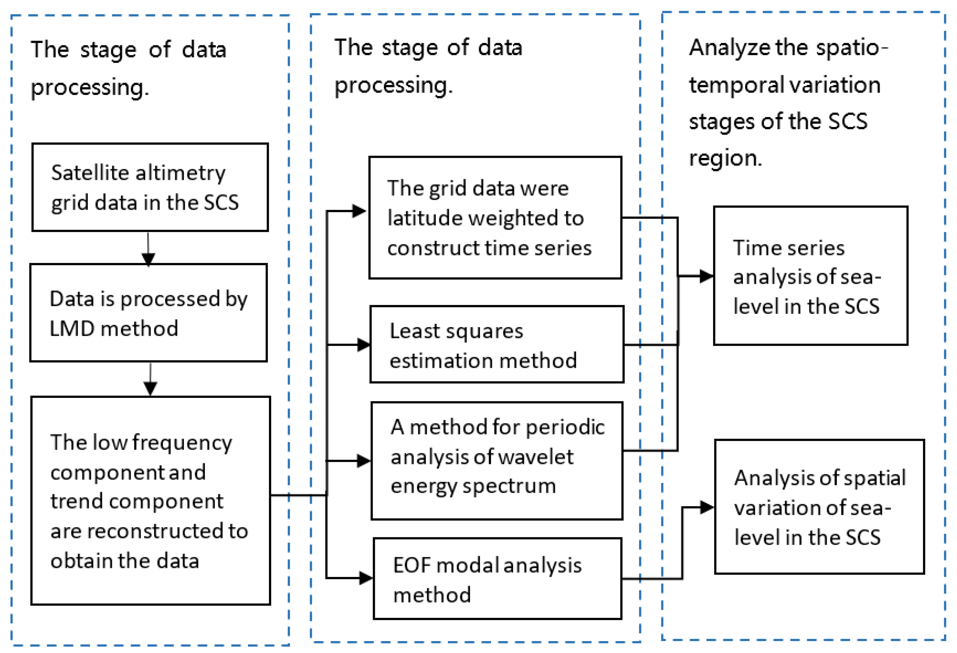
2. Materials and Methods

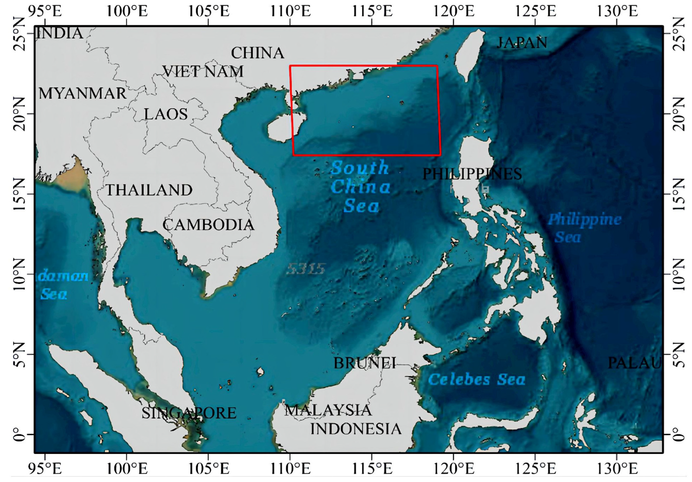
2.1. Adopted Datasets

The South China Sea is located in the center of the Asian–Australian monsoon region, serving as a link between the South Asian monsoon, East Asian monsoon, Northwest Pacific monsoon, and Australian monsoon subsystems. It covers an area of 350,000 square kilometers, with an average depth of 1212 m. To the east, it is adjacent to the Philippines, Palawan, and Kalimantan, and is separated from the Pacific Ocean. To the south, it neighbors the Malay Peninsula, the Natuna Islands, and Kalimantan, and is separated from the Indian Ocean. The South China Sea is the largest tropical marginal sea in the Western Pacific and an important passage connecting the Pacific and Indian Oceans [16,17,18,19,20,21].
The Copernicus Marine Environment Monitoring Service (CMEMS) is the marine component of the European Union’s Copernicus program, providing global data information from satellite observations and remote sensing data worldwide and regionally. This paper uses multi-source satellite gridded fusion altimetry data provided by https://resources.marine.copernicus.eu/ (accessed on 1 May 2021), including data from satellites such as ERS-1/2, TOPEX/Poseidon, GFO, Jason-1/2/3, Envisat, and Sentinel-3A, which have undergone orbit error correction between satellite altimeters and other error corrections, including atmospheric and tidal corrections. The spatial resolution is 1° × 1°, and the time range is from January 1993 to February 2020. The satellite altimetry data within the SCS region range from 110° E to 119° E and 14° N to 23° N (Figure 1).
The LMD method was employed to preprocess the spatiotemporal series of fused satellite altimetry data in the South China Sea region. This involved removing the high-frequency components and subsequently reconstructing a 27-year spatiotemporal series to derive the multi-year average variation in both space and time. To obtain the 27-year time series of sea level change in the entire South China Sea region, the latitudinal weighted method was applied to the temporal and spatial variation series. This approach accounts for the varying latitudinal influence on sea level changes across the region. By performing a periodic analysis of the wavelet energy spectrum, it is possible to extract the periodic characteristics of sea level changes over multiple years. To further investigate the modes of sea level change in the South China Sea, the EOF analysis method was employed to calculate the time coefficients and spatial distributions of different modes. This approach allows for a more comprehensive exploration of the underlying patterns and variations in sea level within the region (Figure 2).

2.2. Local Mean Decomposition Method

Geophysical signals related to sea level change are often nonlinear, nonstationary, and contain multiple frequency components, which are affected by various factors over time [22,23,24,25]. Smith proposed the local mean decomposition (LMD) method in 2005, a method for decomposing data that can analyze the local characteristics of nonlinear, nonstationary signals and better reflect the changing patterns of multiple modes contained in oscillation processes over time and their interrelationships [26]. Considering the characteristics of physical signal changes related to sea level change, this paper adopts the LMD method to extract the signals of sea level change. In this study, the related geophysical signals are denoted as abnormal sea level, and the mentioned signals can also be considered as time series.
The local extremum points and their corresponding time values of the time series, as well as the average values of two adjacent extremum points, are calculated to extract the characteristic information of the data [27]. For the local mean decomposition process of the original signal x ( t ) , the local extremum points are denoted as n i and their corresponding time values as t i , while the average values of two adjacent extremum points n i and n i + 1 are denoted as m i , with the expression given by [28]
m i = n i + n i + 1 2
where m i represents the local mean of the time series, and by extending the m i average value linearly between its corresponding time points, m 11 ( t ) can be obtained. By linear extension, the time series is divided into segments connected by different local means, which are then smoothed. The moving average method is applied to smooth m 11 ( t ) and to obtain the envelope estimation a 11 ( t ) .
Modulation is an important concept in signal processing that can embed the information contained in a signal into another signal. For complex nonstationary time series, the phenomena of amplitude modulation and frequency modulation coexist. Local amplitudes are calculated and modulated, and then frequency modulation is applied to obtain amplitude–frequency-modulated signals [28].
Using the local extremum point a i to calculate the local amplitude, its expression is
a i = n i n i + 1 2
where a i is referred to as the amplitude-modulating signal. Separating the local mean function m 11 ( t ) from the original time series x ( t ) , we obtain [28]
q 11 = x t m 11 ( t )
Next, it is demodulated by dividing q 11 ( t ) by the envelope estimation function a 11 ( t ) to obtain [28]
s 11 t = q 11 t a 11 ( t )
To obtain the pure frequency-modulating signal, the envelope estimation function a 12 ( t ) is computed for s 11 ( t ) . If a 12 ( t ) is not equal to 1, the s 11 ( t ) above iteration process is repeated until s 1 n ( t ) is a pure frequency-modulating signal, i.e., 1 s 1 n ( t ) 1 , and satisfies a 1 n + 1 ( t ) = 1 . Then, we have [28],
  q 11 t = x t m 11 t                         q 12 t = s 11 t m 12 t                     h 1 n t = s 1 n 1 t m 1 n ( t )
The product of all envelope estimation functions generated by the iteration yields the envelope signal a 1 t , which is [28]
a 1 t = a 11 t a 12 t a 1 n t = q = 1 n a 1 q t
Multiplying the function a 1 t represented by the envelope signal product by the pure frequency-modulating signal s 1 n ( t ) , we can express an amplitude–frequency-modulated signal containing amplitude and frequency information. The first PF component can be represented as [28]
P F 1 t = a 1 ( t ) s 1 n ( t )
In the above steps, the first PF component has been separated from the original time series, and the remaining time series can be expressed as u 1 ( t ) , with the loop steps repeated until u k is a monotonic function [28]
u 1 t = x t P F 1 t           u 2 t = u 1 t P F 2 t           u k t = u k 1 t P F k ( t )
Finally, the original time series can be represented as the sum of all PF components and a residual component u k , which is [28]
x t = p = 1 k P F p t + u k
In summary, this method decomposes geophysical signals into a sum of a finite number of PF components and a trend residue u k using LMD.
If the geophysical signal is a time series of sea level changes, the PF components contain low-frequency and high-frequency components, which can be further studied in conjunction with geophysical phenomena. The trend component can be used to estimate the rate of sea level rise.

2.3. Periodicity Analysis Method

The wavelet energy spectrum method can be used to explore the periodic change characteristics of time series. In this paper, wavelet energy spectrum analysis is applied to the sea level change time series [29]. The Morlet wavelet has a good balance in frequency and time scales and is adaptive in multi-scale analysis, so this wavelet was chosen as the basic wavelet [30], with the equation given by
ψ t = π 1 / 4 ( e j w 0 t e w 0 2 2 ) e t 2 2
where ω 0 represents the initial phase angle of the signal, generally taken as ω 0 = 6 .
The equation for the wavelet transform of the time series is [30]
W   f a , b = R f ( t ) ψ ¯ t b a d t
The equation for the wavelet energy spectrum is [30]
E a , b = W f ( a , b ) 2

2.4. Empirical Orthogonal Function (EOF) Analysis Method

Empirical orthogonal function (EOF) is a mathematical statistical method that decomposes the spatiotemporal distribution of variable fields into a linear combination of orthogonal functions called modes by analyzing the structural characteristics of variable fields [31,32,33]. Its purpose is to estimate and interpret the original field using principal component functions and their linear combinations with eigenvectors. The principal components are arranged according to the size of variance contribution and are mutually independent [34]. We suppose there are m variables in a determined range of an element field, observed n times, with the corresponding matrix given by [31]
X = X 11 X 12 X 1 m X 21 X 22 X 2 m X m 1 X m 2 X m m  
Decompose the elements into a linear combination of spatial and temporal functions, with the expression given by [32]
X i j = k = 1 m l i k y k j
where y k j is called the temporal coefficient or the principal component. l i k is called the spatial function, or the coefficient of the principal component, and different spatial functions are orthogonal to each other.

3. Results and Analysis

3.1. Spatial Analysis of Sea Level Change in South China Sea

Using satellite altimetry data ranging from 110° E to 119° E and 14° N to 24° N, the spatial distribution pattern of sea level within the South China Sea region was analyzed. A comprehensive analysis of the overall characteristics of the 27-year sea level spatial distribution in the South China Sea from January 1993 to February 2020 was conducted, as shown in Figure 3 and Figure 4.
From Figure 3, the spatial distributions of average multi-year SCS sea level change can be seen, with a minimum value of 27.72 mm and maximum value of 41.96 mm. Coastal areas, the southern part of the SCS, and the Mindoro Strait have notably greater annual average values, and the SLA in coastal areas is generally greater than that in noncoastal areas. The multi-year average is around 40 mm in the regions of 110° E to 113° E and 14° N to 16° N, and 111° E to 114° E and 20° N to 22° N. In areas close to the central deep-sea basin, east of the Luzon Strait, the Paracel Islands, and the Spratly Islands, the value is around 30 mm within the range of 114° E to 116° E and 16° N to 19° N, and 117° E to 118° E and 14° N to 17° N.
From Figure 4, it can be seen that the smallest multi-year mean sea level change rate in SCS is 2.2 mm/a, and the highest is 4.9 mm/a. A slight decrease in sea level occurs near the east of the Luzon Strait, and the sea level rise rate in coastal areas is faster, with the eastern part of Vietnam experiencing a significant rise. In the regions of 110° E to 113° E and 14° N to 17° N, the sea level change rate is generally greater than 4.0 mm/a, and in the regions of 114° E to 116° E and 16° N to 18° N, the multi-year mean rate is around 3.0 mm/a.

3.1.1. The Seasonal Spatial Patterns of Sea Level Change in the South China Sea

The SCS is the largest semi-enclosed marginal sea basin in the Western Pacific, with significant seasonal change characteristics and prevailing monsoons throughout the year. In the SCS region, the atmosphere transmits signals to the ocean through pressure, forming coupled oscillations, and both influence each other. The seasonal changes in SCS are affected by sea surface atmospheric stress, wind stress, sea surface temperature, the Kuroshio Current, and the ENSO phenomenon. Different seasons have different trends, and there are distinct regional change characteristics. The ENSO phenomenon affects the interaction between the ocean and the atmosphere, forming an ENSO cycle, and can be manifested in mid-to-high latitudes through changes in the Kuroshio Current. Coastal areas in the SCS are usually affected by wind-driven accumulation and thermal expansion, while open sea areas are mainly influenced by the thermal expansion of seawater [35,36,37].
Spring was defined as March to May, summer as June to August, autumn as September to November, and winter as December to February. The spatial variation in the SCS seasonal sea level change from January 1993 to February 2020 was analyzed using satellite altimetry grid data, as shown in Figure 5.
The northeast and southwest monsoons enter the region and are influenced by the Kuroshio Current during spring in the SCS [38]. According to Hung et al. [35], it has been shown that during a warming phase in the spring season in the tropical Western Pacific, the Western Pacific Subtropical High (WPSH) moves eastward. This phenomenon leads to the occurrence of dual cyclones in the Bay of Bengal and the Sumatra region prior to the onset of the summer monsoon in the South China Sea. It can be seen from Figure 5 that in the central part of the South China Sea, the multi-year mean sea level shows a rising trend, while the coastal area shows a negative sea level. The maximum observed value was 98.98 mm and the minimum was −41.31 mm. In the range from 110° E to 115° E and 14° N to 17° N, sea level generally exceeds 50 mm. This spatial distribution is closely related to the effect of wind stress curl and heat flux on sea level pattern.
During the summer, the southwest monsoon has entered the entire SCS region, and the spatial distributions are completely opposite to those of winter. This study examined the anti-phase characteristics of sea level variations in the South China Sea during winter and summer, which align with the conclusions obtained in Wu et al. [21]. This phenomenon is associated with above-normal rainfall in the southern part of the South China Sea during winter, while above-normal rainfall occurs in the northern part of the South China Sea during summer. The deep-water areas of the SCS exhibit positive anomalies, while the northwest and southwest shelf areas exhibit negative anomalies. Due to the influence of the southwest monsoon on the SCS, the multi-year mean of summer is higher than those of other seasons. The highest sea level change is 161.20 mm, while the lowest value is −115.3 mm.
During the monsoon transition season, the spatial distribution of the South China Sea in autumn exhibits a contrasting pattern compared to that observed in spring. As the southwest monsoon gradually weakens, the sea level in coastal areas gradually rises, and a negative anomaly center appears in the deep-water areas of the central South China Sea. Positive anomalies occur at 116° E to 118° E and 18° N to 21° N, and this phenomenon is related to the seasonal changes in wind stress curl [39]. The highest overall value reaches 173.10 mm, while the lowest reaches 4.9 mm.
Influenced by the cold northeastern winds during winter in SCS, the spatial distribution of sea level shows that the winter sea currents in the SCS should be the strongest cyclonic circulation throughout the year. Huo and Yang [39] pointed out that the basin-scale surface circulation in the SCS is predominantly marked by a negative sea surface height anomaly (SSHA), which is closely related to cyclonic activity during winter. In contrast, during summer, the same area exhibits a positive SSHA resulting from anti-cyclonic conditions. Moreover, the center of cyclonic force was situated in the northwestern part of Luzon Island. Those findings from Huo and Yang [39] are consistent with the results shown in Figure 5, which depict negative anomalies in both the deep-water regions of the South China Sea and the Luzon Strait. The highest overall value is 121.30 mm, while the lowest value is −106.7 mm. In the region of 116° E to 118° E and 16° N to 20° N, the multi-year mean is generally higher than −50 mm. As revealed by Hu et al. [38], during the winter, the circulation patterns in the South China Sea are primarily driven by monsoonal winds. Additionally, these circulation patterns are influenced by various local structures, such as warm currents in the western region, the intrusion of the Kuroshio, and small-scale local eddies.
Overall, the sea level in coastal areas is higher in autumn and winter than in spring and summer, and the spatial distribution in spring and autumn, as well as summer and winter, presents largely opposite situations. The spatial distributions of SCS linear trend for four seasons are shown in Figure 6.
For four seasons, there exist some significant differences for the location of maximum change rates. For example, the sea level rise rates near the Paracel and Spratly Islands are higher than other areas in the SCS during the spring season, reaching a maximum of 5.32 mm/a. However, the sea level rise rates near Scarborough Shoal are relatively high, with the highest reaching 5.89 mm/a. Moreover, the sea level rise rate is lower than in other seasons during the winter season in the SCS. Based on a thorough review of the relevant literature, we can observe that sea level changes in the SCS exhibit significant seasonal variations. These variations are influenced by various factors, including topography, ocean circulation patterns, and atmospheric condition [40,41,42,43], which was confirmed by Guo et al. [9]. According to the reference, during winter, there is a positive sea level change in the southwestern part of Taiwan Island, extending northwards, and a negative sea level change in the northwest direction of Luzon Island, extending southwards, which acts as a pumping effect. This phenomenon is related to the westward intrusion of the Kuroshio into the SCS. By analyzing the spatial distribution of average altimetry change rates in each season, it can be concluded that the sea level rise rates in spring and winter are normally lower than summer and autumn, the coastal areas in the SCS have higher rise rates in autumn than the other seasons, and multiple areas in the SCS exhibit rapid sea level rise in the summer [44].

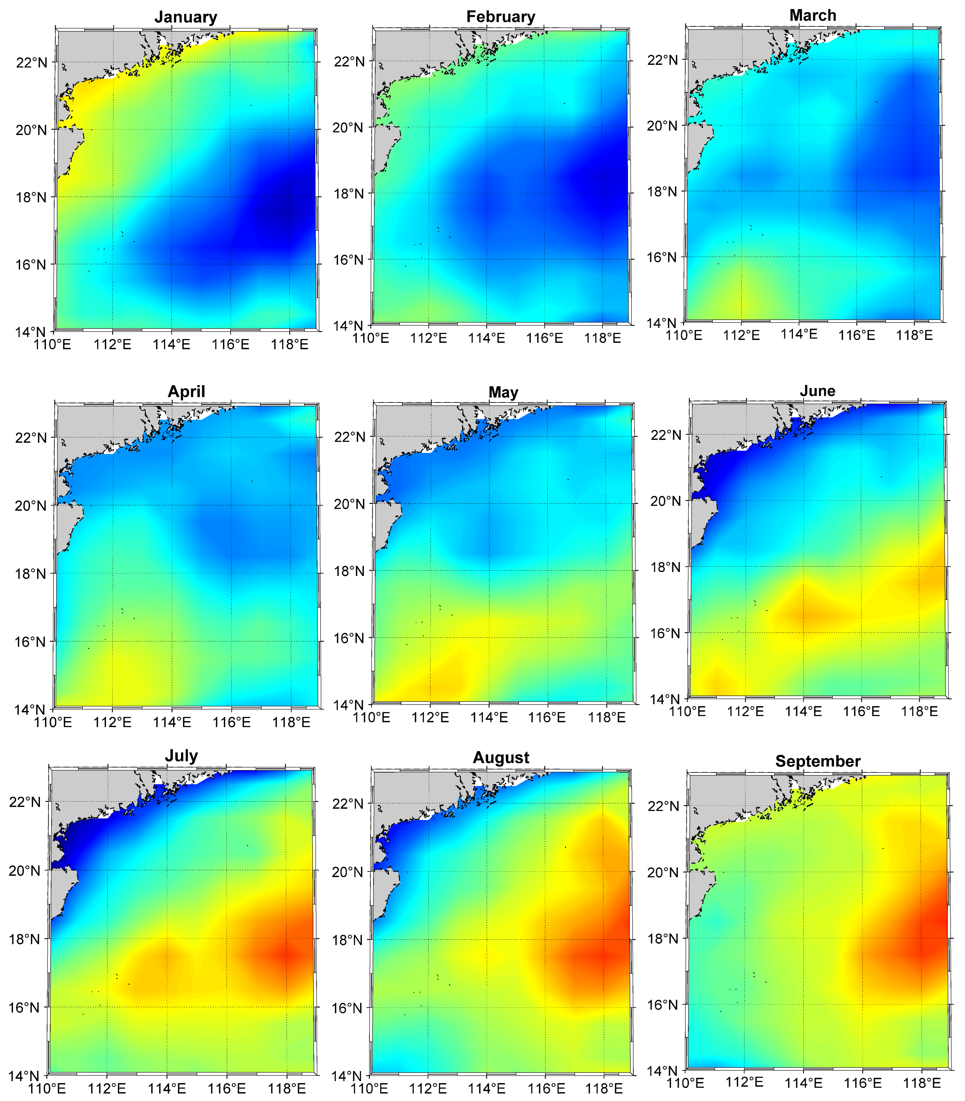
3.1.2. The Monthly Spatial Patterns of Sea Level Change in the South China Sea

Using multi-source satellite altimetry data from January 1993 to February 2020, the spatial patterns of monthly mean sea level change in SCS are presented in Figure 7. We can find that the spatial distributions of the SCS sea level change exhibited significant monthly differences over the 12 months. In January, coastal cities near Hainan, Hong Kong, and Macau generally had sea levels higher than 50 mm, with the highest value in these cities being 118.2 mm and the lowest being −127.00 mm. The northeast wind in the southwest direction raised the high sea level by 40 mm during February. With the intrusion of the Kuroshio Current, there exist significant spatial patterns for the following two months: March and April. However, the southeast monsoon contributed greatly to those spatial patterns of sea level change in the South China Sea from April to November [45,46]. The results comprehensively indicate that the 12-month multi-year mean spatial distribution in the SCS region is influenced by the region’s seasonal changes. Due to the effect of the Kuroshio Current, there are significant local changes in March, April, and May. Due to temperature and climate influences, January, February, October, November, and December have higher average values in coastal areas than other months and more negative average values in the SCS region. Under the influence of the warm and humid monsoon, the overall multi-year mean in June, July, August, and September is higher than in other months.
The results showed that the spatial distribution of SCS sea level change exhibited some significant differences among the 12 months. Coastal cities near Hainan, Hong Kong, and Macau generally had sea levels higher than 50 mm in January. The SCS sea level near the Paracel Islands and Woody Island rose to more than 40 mm due to the northeast wind moving in the southwest direction in February. The SCS sea level in coastal cities near Hainan, Hong Kong, and Macau decreased several folds in February compared with January. The area with negative SLA in the SCS region increased and the sea level of coastal cities near Hainan, Hong Kong, and Macau increased to approximately 10 mm in March and April due to the intrusion of the Kuroshio Current. The seawater moved towards the northwest in May due to the southwest monsoon, resulting in an increase in the sea level near the Zhongsha Islands. The southwest monsoon caused an increase in the sea level in June to August. The effect of the southwest monsoon gradually weakened in September, resulting in an overall decline in the sea level of the South China Sea region [47,48]. The sea level of coastal cities near Hainan, Hong Kong, and Macau was generally higher than 150 mm in October, and the areas with negative values increased. The sea level in the southwestern region declined in November and December due to the effect of the northeast monsoon.
The results comprehensively indicate that the 12-month multi-year mean spatial distribution in the SCS region is influenced by the region’s seasonal changes. Due to the influence of the Kuroshio Current, there are significant local changes in March, April, and May. Due to temperature and climate influences, January, February, October, November, and December have higher multi-year means in coastal areas than other months and more negative values in the SCS. Under the influence of the warm and humid monsoon, the overall value in June, July, August, and September is higher than in other months.

3.2. A Temporal Analysis of Sea Level Change in the South China Sea

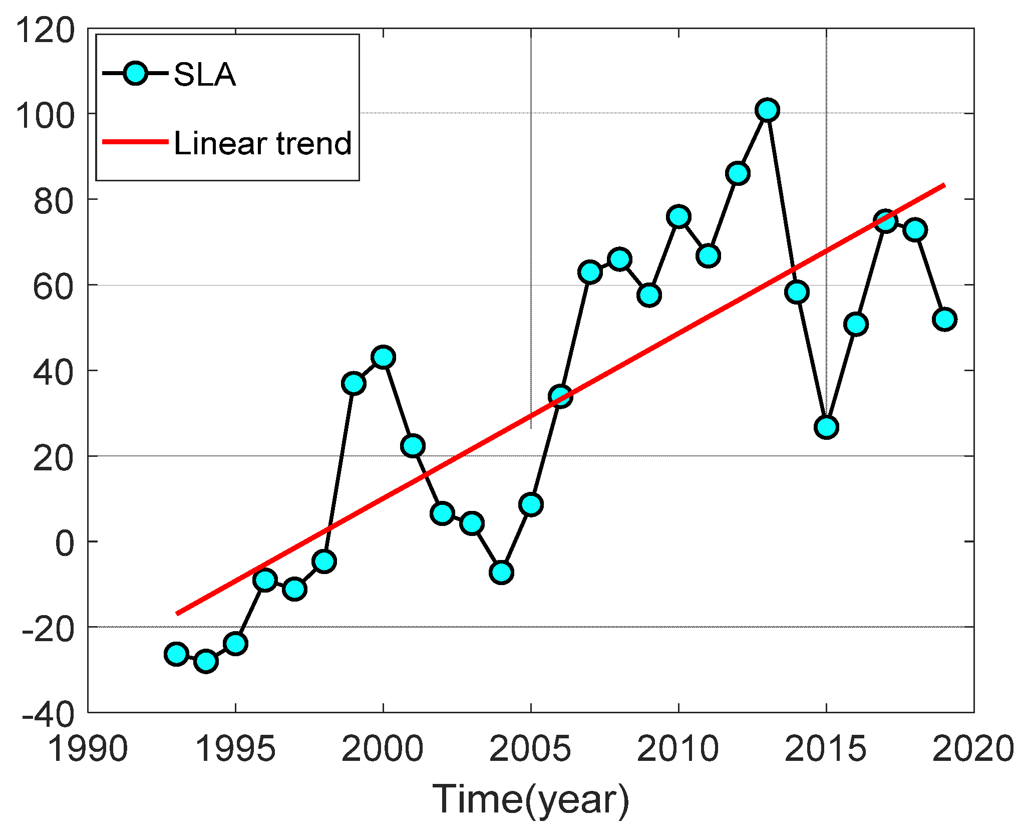
3.2.1. Monthly Mean Sea Level Change in the South China Sea

Monthly mean sea level change is calculated using the weighted average method based on the cosine value of φ (latitude), and the change in monthly mean sea level is obtained, as shown in Figure 8.
The least squares fitting method is then used to estimate the linear trend in SCS regional sea level change.
y = A + B t + C cos ( 2 π ω t + β )
where y represents the alteration in sea level; A denotes the constant component; B signifies the long-term trend element; t symbolizes time; C embodies the amplitude; ω characterizes the period; and β represents the phase.
By employing the local mean decomposition method to eliminate the influence of the PF high-frequency component and retain the trend component and low-frequency component, the yearly time series of the SCS regional mean sea level change was reconstructed, and its linear trend was estimated. The results are shown in Figure 9.
It was concluded that the average of SCS multi-year sea level change was 50.16 mm, with a linear trend of 3.91 ± 0.12 mm/a during the period of 1993–2020, which is close to 4.00 mm/a of the SCS regional mean sea level change rate for the period from 1993 to 2017 [14]. It reached a maximum of 100.18 mm in 2013 and a minimum of −7.23 mm in 2004 over the 27 years. According to Han and Huang [19], the low-frequency component of sea level variations in the South China Sea is more significantly influenced by the El Niño–Southern Oscillation (ENSO) at inter-annual scales. Therefore, we focused primarily on examining the relationship between annual mean sea level changes in the SCS and ENSO index.
The year 1998 was the mature period of a strong La Niña event, and a 32-month La Niña phenomenon occurred from 1998 to 2001. The SCS sea level continuously declined by 50.33 mm from 2000 to 2004. A 23-month La Niña phenomenon occurred from 2010 to 2012, and the SCS sea level continuously declined by 74.08 mm from 2013 to 2015. The results indicate that a long-lasting La Niña phenomenon leads to a significant decline in the SCS, and the change in SCS sea level has a certain lag in time.
The year 1997 was the mature period of a strong El Niño event, and a 13-month El Niño phenomenon occurred from 1997 to 1998. The SCS sea level continuously rose by 47.75 mm from 1998 to 2000. A 13-month El Niño phenomenon occurred again from 1997 to 1998, and the SCS sea level continuously rose by 47.75 mm from 1998 to 2000. A 19-month El Niño phenomenon occurred from 2014 to 2016, and the SCS sea level continuously rose by 48.12 mm from 2015 to 2017.
The comprehensive results demonstrate that a long-lasting El Niño phenomenon leads to a significant increase in SCS, with the changes in sea level exhibiting a certain time lag. This suggests that the method adopted in this study to obtain the yearly SCS mean sea level change series in the SCS is superior to traditional methods for extracting the low-frequency components of sea level change. The analysis of sea level changes and predictions of future sea levels are of practical significance.

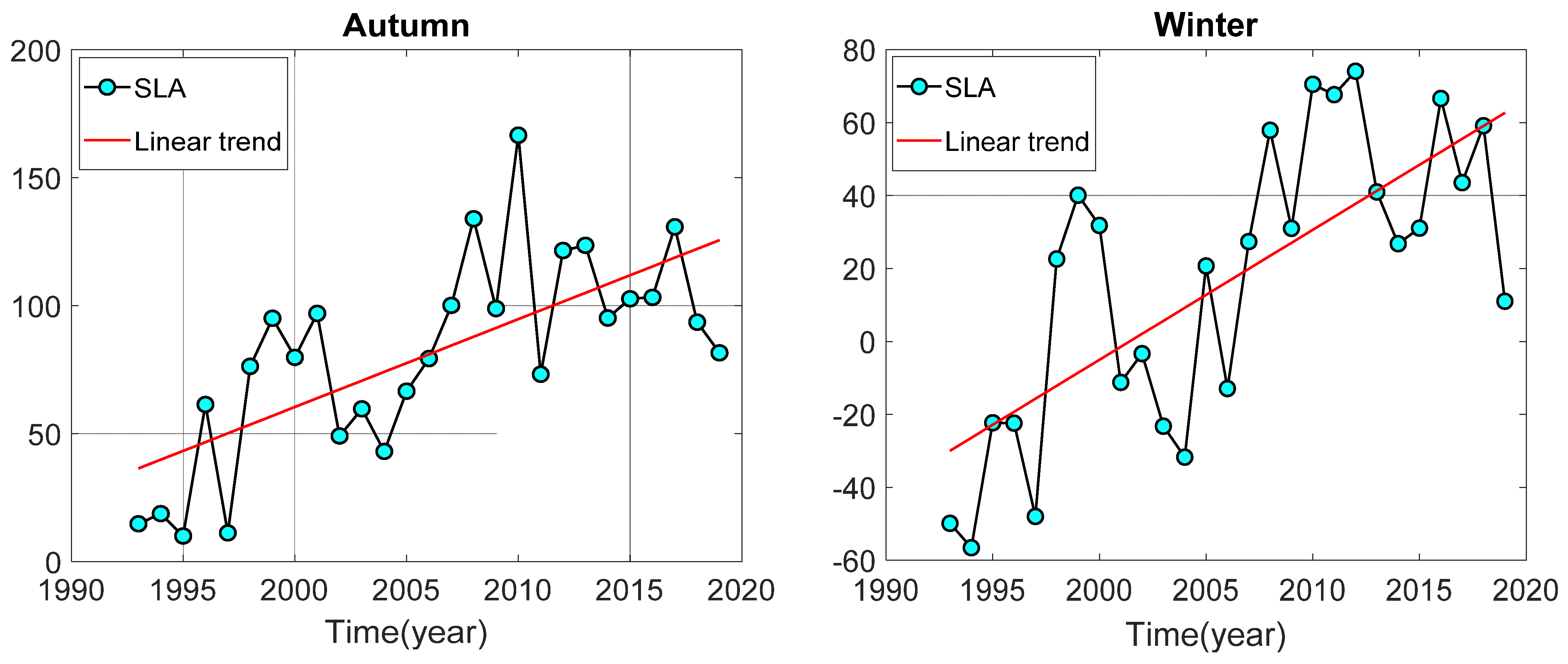
3.2.2. Seasonal Mean Sea Level Change in the South China Sea

The multi-year mean SCS sea level change and its rising rate can be obtained from gridded data over the different timespans. Therefore, examining the multi-year changes in the four seasons of the South China Sea enables a more comprehensive analysis of the underlying causes by considering the seasonal differences. To analyze the temporal variations and linear trends in the seasonal sea level change series in the SCS, the local mean decomposition method was employed to remove the influence of PF high-frequency components while retaining low-frequency components and trend components. The LMD method can decompose the low-frequency components with physical significance, which are the important components related to geophysical information in sea level change. The trend component represents a nonlinear time series of persistent sea level rise. The yearly SCS mean sea level change series in the SCS of four seasons were obtained, respectively, after the reconstruction of the trend component and the low frequency component, and their linear trends were estimated. The results are shown in Figure 10.
The results showed that the yearly mean changes in four seasons exhibited distinct seasonal characteristics over the study period. The results obtained by fitting the least squares method are shown in Table 1.
The multi-year mean of the SCS sea level change was 48.33 mm, with a linear trend of 3.70 ± 0.13 mm/a during the spring season. The multi-year mean was −73.07 mm in the spring season of 1993, whereas the sea level change exhibited a maximum value of 79.60 mm in 2012, with an increase in SCS sea level change of 152.67 mm. The sea level exhibited a sudden and significant rise during the spring season in 1998, 2005, and 2011, followed by a continuous decline from 2012 to 2015.
The average SCS sea level change was 47.71 mm, with an increase rate of 3.66 ± 0.16 mm/a during the summer season. The maximum sea level change during the summer period was 130.70 mm in 2013, with an overall increase of 152.93 mm. The sea level exhibited a sudden and significant rise in 2005 and 2011 during the summer, and a continuous increase from 1994 to 1998. The average SCS sea level change was 44.66 mm during the autumn season, with a rising rate of 3.49 ± 0.16 mm/a. The sea level changes exhibited a sudden and significant increase in the autumn of 1995 and 2004, followed by a consistent increase from 2004 to 2008 during the autumn season. The average SCS sea level change was 46.33 mm during the winter season, with an increase rate of 3.74 ± 0.33 mm/a.
The comprehensive results indicate that, influenced by climate changes such as temperature and precipitation, sea levels in winter and spring are generally lower than those in summer and autumn. Among these, the rate of increase in sea level is the lowest in autumn, and the average value range of sea level changes is the lowest in winter. To analyze the period and amplitude changes of the monthly SCS mean SLA time series, the local mean decomposition method was employed to remove high-frequency components and trend components, followed by anomaly transformation and time series reconstruction, with the results shown in Figure 11a. Wavelet analysis was conducted on this reconstructed time series, with the results shown in Figure 11b,c.
Figure 11 reveals that the wavelet energy spectrum reflects the presence of significant annual fluctuation signals with strong energy in SCS monthly mean SLA time series containing obvious periodic signals. Between 2009 and 2011, there are more prominent annual periodic signals with strong energy. The main periodic terms are 1 year and 1.5 years.

3.3. Modal Analysis of Mean Sea Level Change in the South China Sea

The EOF method describes the space of each mode by decomposing the data of the spatiotemporal distribution variable field into the linear combination of orthogonal functions of the corresponding modes. To study the structural features of the SCS multi-year mean from January 1993 to February 2020, the empirical orthogonal function (EOF) method was utilized to analyze the first three modes that contain 71.33% of the information in the SCS multi-year mean. The results are shown in Figure 12.
Figure 12 illustrates the spatial distribution of the modes and their corresponding time coefficients for the SCS mean sea level. The first mode accounts for 34.09% of the variance in SCS mean changes, the second mode accounts for 28.84%, and the third mode accounts for 8.40%. In terms of the modes’ shapes, the first mode is usually the ENSO mode, with its spatial distribution indicating that the ENSO phenomenon mainly affects the region from 116° E to 120° E and 14° N to 20° N. Comparing this with the spatial distribution of sea level in the SCS region shown in Figure 5, it can be inferred that the second mode is related to the seasonal changes in monsoons, rainfall, and the Kuroshio Current within the SCS region [49]. The spatial distribution of the third mode exhibits a certain similarity to the double-gyre structure of the SCS sea surface temperature, with an increase in sea level in the northeastern region and a declining trend along the coast and in the southwestern region [50,51,52].

4. Conclusions

From 1993 to 2020, the multi-year mean sea level in the SCS was 50.16 mm, with a rate of rise of 3.91 ± 0.12 mm/a. Specifically, during spring, the mean value was 48.33 mm with a change rate of 3.70 ± 0.13 mm/a; during summer, it was 47.71 mm with a change rate of 3.66 ± 0.16 mm/a; during autumn, it was 44.66 mm with a change rate of 3.49 ± 0.16 mm/a; and during winter, it was 46.33 mm with a change rate of 3.74 ± 0.33 mm/a.
Spatial analysis of the multi-year mean, seasonal multi-year mean, and monthly multi-year mean sea levels in the SCS revealed significant spatial variations in the patterns of change. The lowest value observed in the SCS was 27.72 mm, while the highest was 41.96 mm. The lowest change rate recorded was 2.2 mm/a, while the highest was 4.9 mm/a. The sea level rising rates varied across different grid cells in the SCS, with an overall positive change rate and multiple positive centers. During spring and winter, the sea level rise was lower compared to summer and autumn. Coastal regions experienced higher rising rates during autumn, while multiple areas exhibited rapid rises during the summer. The spatial distribution of the 12 months within the SCS region was influenced by regional seasonal climate variations and factors such as the Kuroshio Current, monsoons, and ENSO events.
Analysis of the periodic characteristics of the SCS sea level revealed a more pronounced annual periodic signal with strong energy between 2009 and 2011, primarily driven by terms of 1 year and 1.5 years. The first three modes contributed to the variance at rates of 34.09%, 28.84%, and 8.40%, respectively, representing modes associated with ENSO events, seasonal changes, and the double-gyre structure of the SCS sea surface temperature.

Author Contributions

Conceptualization, L.X. and S.Z.; methodology, L.X.; validation, F.W.; formal analysis, S.Z.; resources, F.W.; writing—original draft, L.X.; writing—review and editing, Y.J.; visualization, L.X.; supervision, S.Z.; project administration, Y.J. All authors have read and agreed to the published version of the manuscript.

Funding

This work was funded by the National Natural Science Foundation of China (42064001, 42374017).

Institutional Review Board Statement

Not applicable.

Informed Consent Statement

Not applicable.

Data Availability Statement

The satellite data used in this study are available via CMEMS (https://resources.marine.copernicus.eu/, accessed on 1 May 2021). ENSO data are available via the NOAA (https://cpc.ncep.noaa.gov/, accessed on 5 July 2021).

Conflicts of Interest

The authors declare no conflict of interest.

References

  1. Yi, S. Global Sea Level Change. In Application of Satellite Gravimetry to Mass Transports on a Global Scale and the Tibetan Plateau; Springer Theses; Springer: Singapore, 2019. [Google Scholar]
  2. Cazenave, A.; Dieng, H.-B.; Meyssignac, B.; von Schuckmann, K.; Decharme, B.; Berthier, E. The rate of sea-level rise. Nat. Clim. Chang. 2014, 4, 358–361. [Google Scholar] [CrossRef]
  3. Sun, J.; Oey, L.; Xu, F.-H.; Lin, Y.-C. Sea level rise, surface warming, and the weakened buffering ability of South China Sea to strong typhoons in recent decades. Sci. Rep. 2017, 7, 7418. [Google Scholar] [CrossRef]
  4. Chen, R.; Wen, Z.; Lu, R. Interdecadal change on the relationship between the mid-summer temperature in South China and atmospheric circulation and sea surface temperature. Clim. Dyn. 2018, 51, 2113–2126. [Google Scholar] [CrossRef]
  5. Pham, D.T.; Switzer, A.D.; Huerta, G.; Meltzner, A.J.; Nguyen, H.M.; Hill, E.M. Spatiotemporal variations of extreme sea levels around the South China Sea: Assessing the influence of tropical cyclones, monsoons and major climate modes. Nat. Hazards 2019, 98, 969–1001. [Google Scholar] [CrossRef]
  6. Wang, H.; Liu, K.; Wang, A.; Feng, J.; Fan, W.; Liu, Q.; Xu, Y.; Zhang, Z. Regional characteristics of the effects of the El Niño-Southern Oscillation on the sea level in the China Sea. Ocean. Dyn. 2018, 68, 485–495. [Google Scholar] [CrossRef]
  7. Wang, H.; Liu, K.; Gao, Z.; Fan, W.; Liu, S.; Li, J. Characteristics and possible causes of the seasonal sea level anomaly along the South China Sea coast. Acta Oceanol. Sin. 2017, 36, 9–16. [Google Scholar] [CrossRef]
  8. Wang, Z.; Wu, R. Individual and combined impacts of ENSO and East Asian winter monsoon on the South China Sea cold tongue intensity. Clim. Dyn. 2021, 56, 3995–4012. [Google Scholar] [CrossRef]
  9. Guo, J.; Zhang, Z.; Xia, C.; Guo, B. Seasonal characteristics and forcing mechanisms of the surface Kuroshio branch intrusion into the South China Sea. Acta Oceanol. Sin. 2019, 38, 13–21. [Google Scholar] [CrossRef]
  10. Agha Karimi, A. Internal variability role on estimating sea-level acceleration in Fremantle tide gauge station. Front. Earth Sci. 2021, 9, 474. [Google Scholar] [CrossRef]
  11. Kenigson, J.; Han, W. Detecting and understanding the accelerated sea-level rise along the east coast of the United States during recent decades. J. Geophys. Res. Ocean. 2014, 119, 8749–8766. [Google Scholar] [CrossRef]
  12. Fu, Y.; Zhou, X.; Zhou, D.; Li, J.; Zhang, W. Estimation of sea level variability in the South China Sea from satellite altimetry and tide gauge data. Adv. Space Res. 2021, 68, 523–533. [Google Scholar] [CrossRef]
  13. Tang, L.; Chen, M. Temporal and spatial variation characteristics of sea-level in the South China Sea in recent 30 years. J. Zhejiang Norm. Univ. (Nat. Sci.) 2022, 45, 446–454. [Google Scholar]
  14. Yu, R.; Xu, H.; Liu, B. Analysis of Spatial and Temporal Variation of sea-level in South China Sea Based on Satellite Altimeter Data. J. Ocean. Technol. 2021, 40, 102–433. [Google Scholar]
  15. Chi, Q. Optimization and Application of Endpoint Effects in Local Mean Decomposition; East China University of Technology: Nanchang, China, 2017. [Google Scholar]
  16. Zhou, L.T.; Tam, C.Y.; Zhou, W.; Chan, J.C. Influence of South China Sea SST and the ENSO on winter rainfall over South China. Adv. Atmos. Sci. 2010, 27, 832–844. [Google Scholar] [CrossRef]
  17. Rong, Z.; Liu, Y.; Zong, H.; Cheng, Y. Interannual sea level variability in the South China Sea and its response to ENSO. Glob. Planet. Chang. 2007, 55, 257–272. [Google Scholar] [CrossRef]
  18. Wang, C.; Wang, W.; Wang, D.; Wang, Q. Interannual variability of the South China Sea associated with El Niño. J. Geophys. Res. Ocean. 2006, 111. [Google Scholar] [CrossRef]
  19. Piton, V.; Delcroix, T. Seasonal and interannual (ENSO) climate variabilities and trends in the South China Sea over the last three decades. Ocean. Sci. Discuss. 2018. [Google Scholar] [CrossRef]
  20. Chao, S.Y.; Shaw, P.T.; Wu, S.Y. El Niño modulation of the South China sea circulation. Prog. Oceanogr. 1996, 38, 51–93. [Google Scholar] [CrossRef]
  21. Wu, R.; Huang, G.; Du, Z.; Hu, K. Cross-season relation of the South China Sea precipitation variability between winter and summer. Clim. Dyn. 2014, 43, 193–207. [Google Scholar] [CrossRef]
  22. Huang, N.E.; Shen, Z.; Long, S.R.; Wu, M.C.; Shih, H.H.; Zheng, Q.; Yen, N.-C.; Tung, C.C.; Liu, H.H. The empirical mode decomposition and the Hilbert spectrum for nonlinear and non-stationary time series analysis. Lond. R. Soc. Lond. 1998, 454, 903–995. [Google Scholar] [CrossRef]
  23. Saramul, S.; Ezer, T. Spatial variations of sea level along the coast of Thailand: Impacts of extreme land subsidence, earthquakes and the seasonal monsoon. Glob. Planet. Chang. 2014, 122, 70–81. [Google Scholar] [CrossRef]
  24. Veltcheva, A.; Soares, C. Nonlinearity of abnormal waves by the Hilbert-Huang Transform method. Ocean. Eng. 2016, 115, 30–38. [Google Scholar] [CrossRef]
  25. Schlurmann, T. Spectral analysis of nonlinear water waves based on the Hilbert-Huang transformation. J. Offshore Mech. Arct. Eng. 2002, 124, 22–27. [Google Scholar] [CrossRef]
  26. Smith, J.S. The local mean decomposition and its application to EEG perception data. J. R. Soc. Interface 2005, 2, 443–454. [Google Scholar] [CrossRef] [PubMed]
  27. Shabbir, M.; Chand, S.; Iqbal, F. Prediction of river inflow of the major tributaries of Indus river basin using hybrids of EEMD and LMD methods. Arab. J. Geosci. 2023, 16, 257. [Google Scholar] [CrossRef]
  28. An, F.P.; Liu, Z.W. Image Processing Algorithm Based on Bi-dimensional Local Mean Decomposition. J. Math. Imaging Vis. 2019, 61, 1243–1257. [Google Scholar] [CrossRef]
  29. Torrence, C.; Compo, G.P. A practical guide to wavelet analysis. Bull. Am. Meteor. Soc. 1998, 79, 61–78. [Google Scholar] [CrossRef]
  30. Santos, C.A.G.; Kisi, O.; da Silva, R.M.; Zounemat-Kermani, M. Wavelet-based variability on streamflow at 40-year timescale in the Black Sea region of Turkey. Arab. J. Geosci. 2018, 11, 169. [Google Scholar] [CrossRef]
  31. Hamlington, B.D.; Leben, R.R.; Strassburg, M.W.; Nerem, R.S.; Kim, K. Contribution of the Pacific Decadal Oscillation to global mean sea-level trends. Geophys. Res. Lett. 2013, 40, 5171–5175. [Google Scholar] [CrossRef]
  32. Nerem, R.; Rachlin, K.; Beckley, B. Characterization of global mean sea level variations observed by TOPEX/POSEIDON using empirical orthogonal functions. Surv. Geophys. 1997, 18, 293–302. [Google Scholar] [CrossRef]
  33. Han, W.; Meehl, G.A.; Stammer, D.; Hu, A.; Hamlington, B.; Kenigson, J.; Palanisamy, H.; Thompson, P. Spatial patterns of sea level variability associated with natural internal climate modes. In Integrative Study of the Mean Sea-Level and Its Components; Springer: Berlin/Heidelberg, Germany, 2017; pp. 221–254. [Google Scholar]
  34. Zhan, J.G.; Wang, Y.; Xu, H.Z.; Hao, X.G.; Liu, L.T. The Wavelet Analysis of sea level Change in China Sea during 1992~2006. Acta Geod. Cartogr. Sin. 2008, 37, 438–443. [Google Scholar]
  35. Hung, R.; Gu, L.; Zhou, L.; Wu, S. Impact of the thermal state of the tropical western Pacific on onset date and process of the South China Sea summer monsoon. Adv. Atmos. Sci. 2006, 23, 909–924. [Google Scholar] [CrossRef]
  36. Han, G.; Huang, W. Low-frequency sea level variability in the South China Sea and its relationship to ENSO. Theor. Appl. Climatol. 2009, 97, 41–52. [Google Scholar] [CrossRef]
  37. Zhang, Y.; Li, J.; Xue, J.; Zheng, F.; Wu, R.; Ha, K.-J.; Feng, J. The relative roles of the South China Sea summer monsoon and ENSO in the Indian Ocean dipole development. Clim. Dyn. 2019, 53, 6665–6680. [Google Scholar] [CrossRef]
  38. Hu, J.; Kawamura, H.; Hong, H.; Qi, Y. A Review on the Currents in the South China Sea: Seasonal Circulation, South China Sea Warm Current and Kuroshio Intrusion. J. Oceanogr. 2000, 56, 607–624. [Google Scholar] [CrossRef]
  39. Huo, D.; Yang, T. Seismic ambient noise around the South China Sea: Seasonal and spatial variations, and implications for its climate and surface circulation. Mar. Geophys. Res. 2013, 34, 449–459. [Google Scholar] [CrossRef]
  40. Chen, J.; Wen, Z.; Wu, R.; Chen, Z.; Zhao, P. Interdecadal changes in the relationship between Southern China winter-spring precipitation and ENSO. Clim. Dyn. 2014, 43, 1327–1338. [Google Scholar] [CrossRef]
  41. Kajikawa, Y.; Wang, B. Interdecadal change of the South China Sea summer monsoon onset. J. Clim. 2012, 25, 3207–3218. [Google Scholar] [CrossRef]
  42. Fang, G.; Wei, Z.; Fang, Y.; Wang, K.; Choi, B. Mean sea surface heights of the South and East China Seas from ocean circulation model and geodetic leveling. Chin. Sci. Bull. 2002, 47, 326–329. [Google Scholar] [CrossRef]
  43. Chao, S.Y.; Shaw, P.T.; Wang, J. Wind relaxation as possible cause of the South China Sea Warm Current. J. Oceanogr. 1995, 51, 111–132. [Google Scholar] [CrossRef]
  44. Jang, H.-Y.; Yeh, S.-W.; Chang, E.-C.; Kim, B.-M. Evidence of the observed change in the atmosphere–ocean interactions over the South China Sea during summer in a regional climate model. Meteorol. Atmos. Phys. 2016, 128, 639–648. [Google Scholar] [CrossRef]
  45. Ichikawa, K. Remote Sensing of the Kuroshio Current System. In Remote Sensing of the Asian Seas; Barale, V., Gade, M., Eds.; Springer: Cham, Switzerland, 2019. [Google Scholar]
  46. Zhang, Q.-H.; Fan, H.-M.; Qu, Y.-Y. Kuroshio Intrusion into the South China Sea. J. Hydrodyn. 2006, 18, 702–713. [Google Scholar] [CrossRef]
  47. Qiu, F.; Pan, A.; Zhang, S.; Cha, J.; Sun, H. Sea surface temperature anomalies in the South China Sea during mature phase of ENSO. Chin. J. Ocean. Limnol. 2016, 34, 577–584. [Google Scholar] [CrossRef]
  48. Wu, C.-R.; Wang, Y.-L.; Lin, Y.-F.; Chao, S.-Y. IIntrusion of the Kuroshio into the South and East China Seas. Sci. Rep. 2017, 7, 7895. [Google Scholar] [CrossRef]
  49. Chen, Y.; Zhao, Y.; Feng, J.; Wang, F. ENSO cycle and climate anomaly in China. Chin. J. Ocean. Limnol. 2012, 30, 985–1000. [Google Scholar] [CrossRef]
  50. Wu, W.; Liu, M.; Yu, S.; Wang, Y. Current Model Analysis of South China Sea Based on Empirical Orthogonal Function (EOF) Decomposition and Prototype Monitoring Data. J. Ocean Univ. China 2019, 18, 305–316. [Google Scholar] [CrossRef]
  51. Guo, J.; Fang, W.; Fang, G.; Chen, H. Variability of surface circulation in the South China Sea from satellite altimeter data. Chin. Sci. Bull. 2006, 51 (Suppl. 2), 1–8. [Google Scholar] [CrossRef]
  52. He, X.; Chen, Z.; Lu, Y.; Zhang, W.; Yu, K. Spatio-temporal Variations of Sea Surface Wind in Coral Reef Regions over the South China Sea from 1988 to 2017. Chin. Geogr. Sci. 2021, 31, 522–538. [Google Scholar] [CrossRef]
Figure 1. The map of the South China Sea area studied in this paper.
Jmse 11 02360 g001
Figure 2. Overall technical roadmap of the paper.
Jmse 11 02360 g002
Figure 3. The spatial distribution of average multi-year SCS SLA (unit: mm).
Jmse 11 02360 g003
Figure 4. The spatial distributions of linear trend in the SCS (unit: mm/a).
Jmse 11 02360 g004
Figure 5. Spatial distribution of seasonal multi-year mean in South China Sea (unit: mm).
Jmse 11 02360 g005
Figure 6. Spatial distribution of seasonal linear trend in South China Sea (unit: mm/a).
Jmse 11 02360 g006
Figure 7. Spatial distribution of monthly multi-year mean in South China Sea (unit: mm).
Jmse 11 02360 g007aJmse 11 02360 g007b
Figure 8. Monthly time series of sea level linear trend in South China Sea.
Jmse 11 02360 g008
Figure 9. Annual time series of sea level change and its change in South China Sea (unit: mm).
Jmse 11 02360 g009
Figure 10. Time series of seasonal multi-year mean linear trends in South China Sea (unit: mm).
Jmse 11 02360 g010aJmse 11 02360 g010b
Figure 11. Wavelet analysis of low-frequency components of sea level in South China Sea. (a) Low-frequency components of sea level in the South China Sea (unit: mm). (b) Wavelet analysis periodogram. (c) Amplitude (unit: mm). The colors in (b) indicate the results of the hypothesis tests, where the yellow part indicates significant periods of change.
Jmse 11 02360 g011
Figure 12. Mean sea level of the South China Sea analyzed by EOF method.
Jmse 11 02360 g012
Table 1. The linear trend and annual amplitude of sea level changes over four seasons from 1993 to 2020.
SeasonTrend (mm/a)Annual Amplitude (mm)Mean Value (mm)Maximum Value (mm)Time of Maximum (year)
Spring3.70 ± 0.1310.93 ± 0.15−48.3379.602012
Summer3.66 ± 0.1618.99 ± 0.1947.71130.672013
Autumn3.49 ± 0.1617.49 ± 0.0844.66166.622009
Winter3.74 ± 0.3318.27 ± 0.2746.3374.082012
Disclaimer/Publisher’s Note: The statements, opinions and data contained in all publications are solely those of the individual author(s) and contributor(s) and not of MDPI and/or the editor(s). MDPI and/or the editor(s) disclaim responsibility for any injury to people or property resulting from any ideas, methods, instructions or products referred to in the content.

