Numerical Prediction of Ship Resistance Based on Volume of Fluid Implicit Multi-Step Method

Abstract

The Volume of Fluid (VOF) method is used in two-phase fluid flow problems of ship hydrodynamic calculations, to capture the motion and distribution of the gas–liquid free surface. To ensure solution stability and accuracy, numerical simulations typically require separate mesh refinement for the free surface or a reduced time step, resulting in a significant increase in solution time. This study aims to compare the drag and vessel attitude change calculations of the VOF implicit multi-step method with the traditional single-step method, and to verify the feasibility of the method in the numerical prediction of ship resistance and flow field analysis. The results show that an implicit multi-step method with a reasonable number of internal iterations could obtain results close to those of the single-step method with a reduced time step, and the error in trim angle was relatively large, about 2%, but the solving time was only about half that of the latter. The method could also capture the shape and location of waves on the hull, especially in the vicinity of the ship, while the distribution of the waves in the far field differed from those in the experiments to some extent.

1. Introduction

The immiscible interface phenomenon is prevalent in marine engineering and plays a significant role in industrial applications involving two-phase fluid flow. The Volume of Fluid (VOF) method [1] is widely used in modeling flow for interface tracking, and is suitable for predicting the distribution and motion of interfaces. During navigation, the existence of a gas–liquid interface affects the motion response and propulsion efficiency of the ship, and, to some extent, the resistance.

Nowadays, reducing carbon emissions and fuel consumption is a pressing issue for the shipping industry; it is related to operating costs and is a requirement of the International Maritime Organization (IMO) for the Environment Ship Index [2], which is a measure of a ship’s compliance with current International Maritime Organization emission standards for reducing air emissions. Therefore, capturing the location and distribution of the free surface around the hull, and predicting the ship resistance accurately and efficiently, is of great importance for ship design and drag reduction.

The ship resistance forecasting methods include model tests and the Computational Fluid Dynamics (CFD) method. Compared to the latter, model tests are widely used and the experimental data are more reliable. When a ship is actually at sea, it is bound to be affected by both air and water resistance. Of these, water resistance can be categorized into calm water resistance and added resistance in waves [3]. Calm water resistance prediction is the estimation of drag force on a ship while moving forward in calm water [4]. Calm water resistance is closely related to the characteristics of the flow field around the ship, and is one of the important factors affecting the speed and energy consumption of the ship. In ship model tests, the resistance is typically treated based on Froude’s method, which divides the drag into the frictional resistance component and residuary resistance component [5]. A DTMB 5415 KCS hull was presented as a standard for examination and verification in Gothenburg [6,7] and Tokyo [8] workshops on CFD in ship hydrodynamics, and detailed experiments were conducted. Simonsen et al. [9] carried out model tests of a KCS hull for hydrostatic and wave conditions in a FORCE Technology towing tank in Denmark. The results of the hydrostatic calculations fitted well with the experimental values. Shivanchev et al. [10] conducted calculations using model tests and numerical methods, to test the additional resistance and ship response under calm and head wave conditions. And the unsteady CFD simulation results were in agreement with the experiments. However, flow field information acquisition is rather complicated and requires considerable time and cost. The short cycle time and fast iteration characteristics of the vessel optimization are not applicable to this scheme.

With the development of high-performance computers, and the gradual improvement of numerical methods and overlapping mesh techniques, direct CFD simulations have provided an approach to solving ship hydrodynamic calculations. Zeng et al. [11] illustrate the effect of curved surfaces on viscous drag in deep water by comparing a two-dimensional flat plate with three ship types, and demonstrate the effect of hull form on viscous drag in shallow water by comparing the Wigley hull, the KCS, and the Rhine 86. Campbell et al. [12], based on STAR-CCM+ software, discussed the effect of trim and draught on resistance in combined water. The influence of free surface on the accuracy of ship resistance should not be neglected. Shia et al. [13] proposed a URANS method for predicting resistance, treating a free surface via the VOF method, and the results for heave, trim, and resistance matched well with the tests. Ilangakoon and Malan [14] provided an approach for calculating high-order accurate curvature (second-order derivative at a point of the surface of a VOF free interface) based on a VOF interface on a non-orthogonal structured grid, which solved the interface curvature analytically. Jeroen et al. [15] discussed the feasibility of adaptive mesh refinement in ISIS-CFD solvers [16,17] applied to resistance predicting, and the results agreed well with experiments and reduced the computation time effectively.

For simulations using the VOF method, other scholars have also conducted different studies on such issues. Liu et al. [18] used a three-dimensional numerical model of six degrees of freedom (DOF) based on the shear stress transport (SST) k-ω eddy viscosity model to capture the complicated characteristics of the vertical water entry of an inclined cylinder at various entry velocities. Wen et al. [19] used a (SST) k-ω model to analyze the attitude and drag of a DTMB-5415 frigate during the steady water entry phase, where the fluid volume method was used to capture the interface between water and air. Zhenming et al. [20] applied a CFD approach combining LES modeling with free surface capture VOF techniques to simulate a primary split in a high-speed diesel jet. Xiaohan et al. [21] used the VOF method to track the inlet process of an ocean submersible buoy, studied the final deployment process of the anchor, and obtained the velocity changes, mechanical behavior, and fluid velocity changes of the three components through numerical simulations.

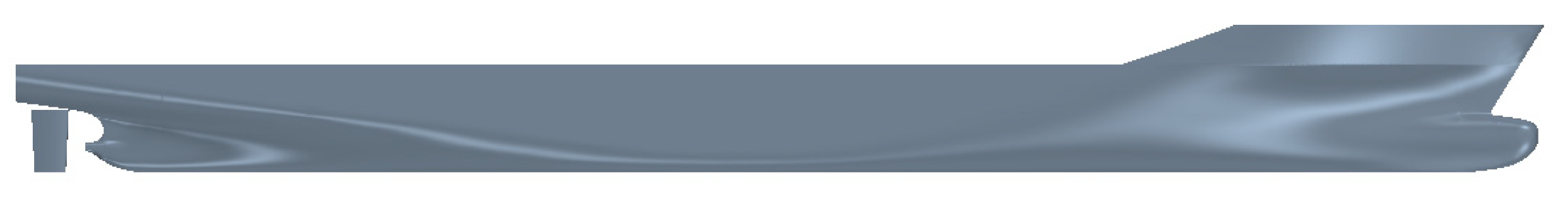
Despite the maturity of research on ship resistance calculations using CFD methods, there is less research related to free surface capture in ship hydrodynamics. This study focuses on the validation and application of the VOF implicit multi-step method to ship resistance predictions. In this paper, numerical simulations of calm water resistance are carried out for a KRISO Container Ship (KCS) model, based on the Unsteady Reynolds-Averaged Navier–Stokes (URANS) method, capturing the location and shape of the free surface using the VOF method. The advantages and limitations of the VOF implicit multi-step method are discussed based on calculations of the resistance and flow field distribution at Fr = 0.260 using both the single-step method and implicit multi-step method.

In addition, the research in this paper concentrates on the usage of the VOF algorithm, meshing and time step, solution time, and error. The Computational Fluid Dynamics method is considered a tool rather than a focused point. Therefore, the adopted methods are only described briefly, and the derivation and expansion are not further elaborated.

2. Ship Geometry and Condition

A KCS ship model (scale ratio of 31.6) appended with a fixed rudder was modeled in this paper. The geometry and main parameters of the hull and rudder are described in Figure 1 and

Table 1. The main particulars of the KCS model.

Main Particulars	Symbols and Units	Values
Scale ratio	λ	31.6
Length between the perpendiculars	LPP (m)	7.2786
Length of waterline	LWL (m)	7.3577
Beam of waterline	BWL (m)	1.019
Draft	D (m)	0.6013
Displacement	Δ (m3)	1.649
Block coefficient	CB	0.6505
Wetted area (with rudder)	S (m2)	9.512
Longitudinal center of buoyance	LCB (%LPP)	−1.48
Radius of gyration	Kxx/B	0.4
Radius of gyration	Kyy/LPP, Kzz/LPP	0.25

.

The ship resistance analysis [22,23] was carried out with reference to a standard example (Case 2.1), shown in

Table 2. The case conditions for the KCS model.

Parameters	Symbols and Units	Values
Density	ρ (kg/m3)	999.5
Kinematic viscosity	v (m2/s)	1.27 × 10−6
Speed	U (m/s)	2.196
Froude number	Fr	0.26
Reynolds number	Re	1.26 × 107

. The condition was chosen for a Froude number of 0.260, corresponding to a speed of 2.196 m/s in model scale. During the calculations, the change in vessel attitude (heave and trim) was taken into account and the position of the rudder was fixed.

3. Numerical Modeling

The predictions of calm water resistance were conducted using commercial CFD software STAR-CCM+, version 17.02.007. This section introduces the specific numerical methods and meshing strategies employed in the CFD simulations.

3.1. Governing Equations

Turbulence is inherently unsteady, but the property is typically centered on a mean value. According to this characteristic, the Unsteady Reynolds-Averaged Navier–Stokes method utilizes statistical steadiness and ensemble averaging to time-average the Navier–Stokes equations. For unsteady incompressible flows, the average continuity and momentum equations in tensor notation and Cartesian coordinates are as follows:

$$\frac{\partial {\overline{u}}_i}{\partial x_i}=0,$$

(1)

$$\rho \frac{\partial {\overline{u}}_i}{\partial t}+\rho {\overline{u}}_j\frac{\partial {\overline{u}}_i}{\partial x_j}=-\frac{\partial \overline{p}}{\partial x_i}+\frac{\partial }{\partial x_j}(2\mu {\overline{s}}_{ij}-\rho {\overline{{u^{\prime }}_j{u}^{\prime }}}_i),$$

(2)

$${\overline{s}}_{ij}=\frac{1}{2}(\frac{\partial {\overline{u}}_i}{\partial x_j}+\frac{\partial {\overline{u}}_j}{\partial x_i}),$$

(3)

where $\rho$ is the fluid density, ${\overline{u}}_i$ is the averaged velocity vector, $\overline{{u^{\prime }}_j{u^{\prime }}_i}$ is the Reynolds stress tensor term, and ${\overline{s}}_{ij}$ is the Reynolds-averaged version of the strain-rate tensor.

From Equations (1) and (2), there are ten unknowns in the three-dimensional problem. To solve these equations, it is necessary to devise a closure for the system, which is referred to as a turbulence closure model (TCM). The turbulence model in this paper is based on the Boussinesq eddy-viscosity assumption, and the expressions are defined as follows:

$$-\rho {\overline{{u^{\prime }}_i{u}^{\prime }}}_j=2{\mu }_t{\overline{s}}_{ij}-\frac{2}{3}\rho {\delta }_{ij}k,$$

(4)

where ${\mu }_t$ is the eddy viscosity, ${\delta }_{ij}$ is the Kronecker-delta function, and k is the turbulent kinetic energy.

The turbulence models applied in this paper are based on the Boussinesq eddy-viscosity assumption, which is based on the link between viscosity and turbulence: turbulence leads to dissipation and transport of mass, momentum, and energy in directions orthogonal to the streamlines, and the above phenomena are directly related to viscosity. Therefore, many turbulence models are based on the concept of eddy viscosity and the increase in viscosity in turbulence, and the increase in turbulence can also be represented by viscosity. The turbulence confinement models provided in STAR-CCM+ include both RANS turbulence models and scale solver simulations. For the Reynolds-averaged turbulence model, the eddy viscosity model in STAR-CCM solves additional transport equations to obtain the eddy viscosity ${\mu }_t$, such as the Spalart–Allmaras model for the single-equation, the k-ε model for the two-sided equation, and the k-ω model. The k-ε models for two-equation models include Standard k-ε model and Realizable k-ε model. The k-ω models include the Standard k-ω model and SST (Shear Stress Transport) k-ω model.

In this paper, the computational domain was discretized based on the Finite Volume (FV) method, and the discretized governing equations could be solved using a set of finite control volumes that constitute the domain. Each control volume contains nodes under which the flow variables are calculated, and the calculations require surface and volume integration for the corresponding control volume. A second-order accurate method [24] was applied, and we discretized the time in a second-order central difference format.

3.2. Physics Modeling

Shear Stress Transport (SST) k-ω turbulence model [25] was employed in this paper, and an additional cross-diffusion term was added. By combining the k-ε model in the far field and the k-ω model near the wall effectively through a hybrid function, the drawbacks of the k-ω turbulence model applied in real fluid simulations could be resolved. The turbulent kinetic energy k and the unit turbulent dissipation rate ω are defined as follows:

$$\frac{\partial }{\partial t}(\rho k)+\nabla ·(\rho k\bar{v})=\nabla ·\left[\left(\mu +{\sigma }_k{\mu }_t\right)\nabla k\right]+P_k-\rho {\beta }^{*}{f}_{{\beta }^{*}}\left(\omega k-{\omega }_0{k}_0\right)+S_k$$

(5)

$$\frac{\partial }{\partial t}(\rho \omega )+\nabla ·(\rho \omega \bar{v})=\nabla ·\left[\left(\mu +{\sigma }_{\omega }{\mu }_t\right)\nabla \omega \right]+P_{\omega }-\rho \beta f_{\beta }\left({\omega }^2-{\omega }_0^2\right)+S_{\omega }$$

(6)

where $\bar{v}$ is the mean velocity, $\mu$ is the dynamic viscosity, and $f_{\beta }^{\mathrm{*}}$ and $f_{\beta }$ are the free shear and bath extension correction factors, respectively. The resulting terms $P_k$ and $P_{\omega }$ are defined in the SST model as follows:

$$P_k=G_k+G_{nl}+G_b$$

(7)

$$P_{\omega }=G_{\omega }+D_{\omega }$$

(8)

where $G_k$ is the turbulence term, $G_b$ is the buoyancy term, $G_{nl}$ is the nonlinear term, $G_{\omega }$ is the unit dissipation term, and $D_{\omega }$ is the cross-diffusion term.

All-y+ wall treatment was used for the wall function, ensuring that the y+ value was greater than 30 to simulate the flow characteristics near the wall accurately, where y+ is given by the following equation:

$$y^{+}=\frac{\Delta y{u}_r\rho }{u}=\frac{\Delta y}{v}\sqrt{\frac{{\tau }_w}{\rho }}$$

(9)

where $u$ is the time-averaged velocity of the fluid, $u_r$ is the wall friction velocity, and $u_r={\left(\frac{{\tau }_w}{\rho }\right)}^{\frac{1}{2}}$. ${\tau }_w$ is the wall shear stress, and $\mathsf{\Delta }y$ is the distance to the wall (height of the first layer of the mesh).

In STAR-CCM+, the ship motion is achieved through the overset mesh and Dynamic Fluid Body Interaction (DFBI) module, which allows the vessel to move freely or with constraint. When a constraint exists, the constraint will allow some degrees of freedom and limit others. The equations for constrained motion are described as follows:

$$\varphi (d,t)=0,$$

(10)

where t is time, and d is the coordinate vector, defined by $d=(r_x,r_y,r_z,\varphi ,\theta ,\psi )$.

This study investigated the calm water resistance of the KCS hull, which was mainly influenced by the heave and trim with the other degrees of freedom being negligible. Hence, only y-axis rotation and z-axis translation were allowed (marked in red in Figure 2), as shown in Figure 2.

3.2.1. VOF Method

The Volume of Fluid method is generally utilized to predict the distribution and motion of an immiscible interface (e.g., gas and liquid). An important quality of immiscible phases is that fluids are always separated by a sharp interface. With sufficient grid resolution, this method is capable of tracking the shape of the free surface between gas and liquid. The distribution of each phase and the location of the interface are expressed as the volume fraction ${\alpha }_i$, and the transport equation is defined as follows:

$$\frac{\partial }{\partial t}{\displaystyle {\int }_V{\alpha }_{i}dV+{\displaystyle {\oint }_A{\alpha }_{i}vda={\displaystyle {\int }_V(S_{{\alpha }_i}-\frac{{\alpha }_i}{{\rho }_i}\frac{D{\rho }_i}{Dt})dV}}}-{\displaystyle {\int }_V\frac{1}{{\rho }_i}\nabla ({\alpha }_i{\rho }_i{v}_{d,i})}dV,$$

(11)

where a is the area vector, v is the mixed velocity, $v_{d,j}$ is the diffusion velocity, and $S_{{\alpha }_i}$ is the custom source term for phase i.

The continuity, momentum, and energy equations and related expressions for two-phase flow are defined as follows:

$$\frac{\partial }{\partial t}\left({\int }_V\rho dV\right)+{\oint }_A\rho v·da={\int }_{V}SdV$$

(12)

$$\begin{array}{cc}\hfill \frac{\partial }{\partial t}\left({\int }_V\rho vdV\right)+& {\oint }_A\rho v\otimes v·da\hfill \\ & =-{\oint }_{A}pI·da+{\oint }_{A}T·da+{\int }_V\rho gdV+{\int }_V{f}_{b}dV\\ & -{\displaystyle \sum _i}{\int }_A{\alpha }_i{\rho }_i{v}_{d,i}\otimes v_{d,i}·da+{\int }_V{S}_i^{\alpha }dV\end{array}$$

(13)

$$\begin{array}{cc}\hfill \frac{\partial }{\partial t}{\int }_V\rho EdV+{\oint }_A& \left[\rho Hv+{\displaystyle \sum _i}{\alpha }_i{\rho }_i{H}_i{v}_{d,i}\right]·da\hfill \\ & =-{\oint }_A{\dot{q}}^n·da+{\oint }_{A}T·vda+{\int }_V{f}_b·vdV+{\int }_V{S}_{E}dV\end{array}$$

(14)

$$S=\sum _i{S}_{a_i}·{\rho }_i$$

(15)

where S is the mass source term, p is the pressure, I and T are the unit and stress tensors, respectively, f_b is the body force vector, $S_i^a$ is the phase momentum source term, E and H denote the total energy and total enthalpy, respectively, and S_E is the customized energy source term.

The High-Resolution Interface Capturing (HRIC) scheme serves to simulate the convective transport of immiscible phases, and could be used to trace the position of the interface, as shown in Figure 3. The scheme is utilized by the VOF method to obtain an accurate second-order approximation of volume fraction, which is bound by an upper Courant Limit (CFL). When the CFL is exceeded, a first-order upwind scheme is employed to maintain stability, resulting in poor approximation at the interface. The introduction of a time sub-cycle into the volume fraction transport equation could resolve this problem, and improve the resolution of the gas–liquid fluid flow interface.

For a standard FV discrete and time-independent control volume, the integral expression for Equation (11) in arbitrary time intervals is described as follows:

$${\alpha }^{n+\Delta t}V-a^{n}V+{\displaystyle {\int }_{t^n}^{t^n+\Delta t}({\displaystyle {\sum }_A{\alpha }_f(s)vda})ds=}{\displaystyle {\int }_{t^n}^{t^n+\Delta t}(S(\alpha (s),\dots )}ds,$$

(16)

where ${\alpha }_f$ is the face value volume fraction, Δt is the current time step size, and the terms on the right-hand side of Equation (11) are combined into a single source term.

For the VOF single-step solution strategy of the solver, Equation (16) can be written in the following form:

$${\alpha }^{n+\Delta t}V-a^{n}V+\Delta t({\displaystyle {\sum }_A{\alpha }_f^{n+\Delta t}(\Delta t)vda})=\Delta tS({\alpha }^{n+\Delta t},\dots ),$$

(17)

where the face value ${\alpha }_f^{n+△t}$ is obtained from the HRIC solution, and treated implicitly according to time.

To resolve the time step restriction on the global time step size Δt, the multi-step method divides the time interval $[t^n,t^n+\Delta t]$ into N uniform sub-intervals $[t_i,t_{i+1}], i=0, \dots , N-1$, and calculates the intermediate solution for each sub-interval. The strategy of the VOF multi-step method supported in STAR-CCM+ includes both explicit and implicit multi-step methods, defined as follows:

$${\alpha }_{i+1}V-a_{i}V+\tau ({\displaystyle {\sum }_A{\alpha }_{f,i}(\tau )vda})=\tau S({\alpha }^{n+\Delta t},\dots ),$$

(18)

$${\alpha }_{i+1}V-a_{i}V+\tau ({\displaystyle {\sum }_A{\alpha }_{f,i+1}(\tau )vda})=\tau S({\alpha }^{n+\Delta t},\dots ),$$

(19)

In multi-stepping, the solution of the face value ${\alpha }_f$ is subject to the reduced time step size; thus, the upwind-blending corresponding to CFL is reduced. The sum of all sub-time steps gives:

$${\alpha }^{n+\Delta t}V-a^{n}V+{\displaystyle \sum _{i=0}^{N-1}\tau ({\displaystyle {\sum }_A{\alpha }_{f,i(i+1)}(\tau )vda})}=\Delta tS({\alpha }^{n+\Delta t},\dots ),$$

(20)

The stability of the explicit multi-stepping is bounded by the CFL condition ($CFL/N_{\exp }\le 1$). And the VOF explicit multi-step solver determines the number of required sub-steps automatically, and cannot be modified. Therefore, it is not applicable to practical marine engineering. However, implicit multi-stepping is not bound to the time step restriction, and the number of inner iterations could be customized, whereas the solver applies under-relaxed corrections to intermediate solutions. If the sub-time steps exceed the CFL limit of the HRIC scheme, it could lead to diffusion in the solution of the volume fraction.

3.2.2. Mesh Generation

Background and overset domain meshes were generated using the automatic meshing module and trimmed cell mesher in STAR-CCM+. The advantages of this meshing method are that each subdomain mesh is generated individually, the generation of subdomain meshes are not restricted, and the movement of subdomain meshes does not affect the overall mesh. The resulting mesh was stable, efficient, and of high quality, and was appropriate for resolving complex flow characteristics.

The flow separation phenomenon on the hull surface has a significant impact on resistance and pressure drop. To solve the flow characteristics accurately, a prism layer mesh was generated at the near-wall surface that was orthogonal to the boundary to ensure a wall y+ value around 30. Meanwhile, we captured the flow characteristics exactly, especially the location and shape of waves in the bow and stern with free surfaces. Thus, it is necessary to apply appropriate mesh refinement at the corresponding position. Figure 4 shows the layout of the computational domain and the mesh near the hull.

The calculation of ship calm water resistance is symmetrical; in order to improve the computational efficiency, a half domain was adopted for numerical simulations in this paper. The computational domain range was: $-3.0L_{pp}<x<1.0L_{pp}$, $0<y<1.5L_{pp}$, $-1.0L_{pp}<z<0.5L_{pp}$. The origin of the coordinate was located at the intersection of the initial waterline and central axis of the rudder stock, with the bow facing in the positive x direction, as shown in Figure 5. In order to simulate the flow field distribution of the free surface, and analyze the discrepancies between the traditional single-step method and implicit multi-step method, the meshing and boundary condition settings remained the same. The upstream, top, bottom, and side boundaries were set as the velocity inlet, while the downstream and mid-longitudinal profile were set up as the pressure outlet and symmetry, respectively.

For the purpose of avoiding reflections from ship waves reaching the boundary, which affect the accuracy and reliability of the solution, a wave dissipation region (e.g., a force source term) was set up. Forcing the 3D Navier–Stokes equations to obtain a simplified theoretical solution involving wave damping and wave force. In this work, the method proposed by Choi and Yoon [26] was applied, which added an additional drag term to the w-velocity equation to produce wave damping. Figure 6 shows a schematic diagram of the damping zone in the CFD simulations.

4. Results and Discussion

The following section aims to compare and analyze the resistance prediction results and flow field distribution of the VOF implicit multi-step method and Simple-step method. Verification and validation studies are carried out to illustrate the strengths and limitations of free surface capture and the computational cost, and to provide a reference method for ship resistance simulations.

4.1. Verification Study

Before carrying out numerical simulations based on the VOF implicit multi-step method, single-stepping was first employed to examine the flow field calculations considering the heave and trim motion of the KCS model. During the simulations, the model was subjected to ship attitude changes due to hydrodynamic and gravitational forces, and the amplitude of motion decreased until a state of complete equilibrium was reached. The results were also validated against available experimental data (Tokyo 2015), which included calm water resistance and free surface waves.

According to the procedure by Celik et al. [27], the mesh and time step conver-gence study was based on the Grid Convergence Index (GCI) to determine the form of convergence. Fine, medium, and coarse grids were used for validation, and the num-bers of grids were N₁, N₂, and N₃, and the mesh and time step [28] refinement factor r₂₁ are defined as follows:

$$r_{21}=\sqrt[3]{\frac{N_1}{N_2}}$$

(21)

$$r_{21}=\Delta t_2/\Delta t_1$$

(22)

where r₂₁ is the scaling of the grid and time. For the apparent order, p is the order of discretization, and is calculated using Equation (23):

$$p=\frac{1}{\ln (r_{21})}\left|\ln \left|\frac{{\epsilon }_{32}}{{\epsilon }_{21}}\right|+q(p)\right|,$$

(23)

$$q(p)=\ln (\frac{r_{21}^p-s}{r_{32}^p-s}),$$

(24)

$$s=1·\mathrm{sgn}(\frac{{\epsilon }_{32}}{{\epsilon }_{21}}),$$

(25)

where ${\epsilon }_{32}={\varphi }_3-{\varphi }_2$ and ${\epsilon }_{21}={\varphi }_2-{\varphi }_1$ represent the differences between coarse–medium and medium–fine solutions, where ${\varphi }_i$ corresponds to the solution for that grid (i = 1, 2, 3 for fine, medium, and coarse grids, respectively). s = 1 indicates that the results show consistent convergence, and s = −1 indicates that the results show oscillatory convergence. The expression for extrapolated values ${\varphi }_{ext}^{21}$ is described as follows:

$${\varphi }_{ext}^{21}=\frac{r_{21}^p{\varphi }_1-{\varphi }_2}{r_{21}^p-1},$$

(26)

Approximate errors $e_a^{21}$ and extrapolated relative errors $e_{ext}^{21}$ are defined as:

$$e_a^{21}=\left|\frac{{\varphi }_2-{\varphi }_1}{{\varphi }_1}\right|,$$

(27)

$$e_{ext}^{21}=\left|\frac{{\varphi }_{ext}^{12}-{\varphi }_1}{{\varphi }_{ext}^{12}}\right|,$$

(28)

In conclusion, the convergence index $GC{I}_{\mathrm{fine}}^{21}$ of the fine mesh is obtained using the following expression:

$$GC{I}_{fine}^{21}=\frac{1.25e_a^{21}}{r_{21}^p-1}$$

(29)

The primary objects of the convergence study include the resistance coefficient, trim, and heave, which are available through sensors in the model tests.

4.1.1. Spatial Convergence Study

The three resolutions of grids adopted for verification are fine, medium, and coarse grids, corresponding to 4,777,034, 2,151,616, and 1,027,928, respectively.

Table 3. Calculation of the discretization error for the spatial convergence study.

	Resistance Coefficient	Trim	Sinkage
r21	1.30	1.30	1.30
r23	1.28	1.28	1.28
φ1	0.0036944	−0.1740020 deg	−0.0135945 m
φ2	0.0036944	−0.1716800 deg	−0.01359466 m
φ3	0.0036180	−0.1762450 deg	−0.01376446 m
ε32	−7.64 × 10−5	−4.57 × 10−3 deg	−1.70 × 10−4 m
ε21	−3.43 × 10−8	2.32 × 10−3 deg	−1.50 × 10−7 m
s	1	−1	1
q	0.000929%	1.334467%	0.001103%
pa	6.15 × 10−1	3.49 × 10−2	5.61× 10−1
${\phi }_{\mathrm{ext}}^{21}$	3.13 × 101	2.67 × 100	2.86 × 101
${\mathrm{e}}_{\mathrm{ext}}^{21}$	2.00 × 10−9	1.27 × 10−2	6.00 × 10−9
${\mathrm{GCI}}_{\mathrm{fine}}^{21}$	0.0000003%	1.6103827%	0.0000007%

lists the mesh convergence analysis results for the ship resistance simulations, where N₁ = 4,777,034, N₂ = 2,151,616, and N₃ = 1,027,928.

As can be seen from Table 3, the numerical uncertainties for the resistance coefficient, trim and heave are 0.0000003%, 1.6103827%, and 0.0000007%, respectively, with an overall uncertainty of less than 2%.

4.1.2. Temporal Convergence Study

The calculation conditions for the time-step convergence study are similar to the grid convergence, with a Froude number of 0.260 being chosen for the simulations. The time step refinement factor r₂₁ remains constant, with a minimum time step of 0.005 s.

Table 4. Calculation of the discretization error for the temporal convergence study.

	Resistance Coefficient	Trim	Sinkage
r21	2.00	2.00	2.00
r23	2.00	2.00	2.00
φ1	0.0036809	−0.169457 deg	−0.0136624 m
φ2	0.0036944	−0.17168 deg	−0.01359466 m
φ3	0.0037140	−0.170599 deg	−0.0135868 m
ε32	1.95 × 10−5	1.08 × 10−3 deg	7.86 × 10−6 m
ε21	1.35 × 10−5	−2.22 × 10−3 deg	6.77 × 10−5 m
s	1	−1	1
${\mathrm{e}}_{\mathrm{a}}^{21}$	0.367314%	1.311837%	0.495813%
pa	5.32 × 10−1	1.04 × 100	3.11 × 100
${\phi }_{\mathrm{ext}}^{21}$	3.65 × 10−3	−1.67 × 10−1	−1.37 × 10−2
${\mathrm{e}}_{\mathrm{ext}}^{21}$	8.31 × 10−3	1.26 × 10−2	6.50 × 10−4
${\mathrm{GCI}}_{\mathrm{fine}}^{21}$	1.030297%	1.552207%	0.081352%

shows the time discretization errors of the main parameters, where Δt₁ = 0.005 s, Δt₂ = 0.01 s, and Δt₃ = 0.02 s.

As can be seen from Table 4, the numerical uncertainties of 1.030297%, 1.552207%, and 0.081352% were calculated for the numerical resistance coefficient, trim, and heave, respectively, with an overall numerical uncertainty error of less than 2%.

4.2. Validation Study

In the validation study, the subsequent simulations were carried out based on the time step Δt₂, taking into account the computational accuracy and costs. The accuracy of the numerical methods and physical models was verified by comparing the numerical results with the experimental values, to obtain the relative error of the numerical calculations. The results of the validation analysis are shown in

Table 5. Comparison of ship motion and resistance coefficients.

Mesh Type	Resistance Coefficient	Error	Trim (deg)	Error	Sinkage (m)	Error
N1	0.0036944	0.446	−0.1740020	−2.960	−0.01359451	2.478
N2	0.0036944	0.447	−0.1716800	−1.586	−0.01359466	2.477
N3	0.0036180	2.507	−0.1762450	−4.287	−0.01376446	1.259
EFD	0.003711		−0.169		−0.01394

, where EFD is the experimental value.

It can be seen from the results in Table 5 that the numerical calculations of calm water resistance of the KCS hull were in good agreement with the tests. The coarse grid showed a larger error of about 2.5%, while the fine and medium grids were close, within 0.5%. For the ship attitude, the predicted trim and heave of the KCS model basically matched the experimental value, and the results of the fine and medium grids were almost the same, with an error within 3%. The maximum error was about −4.3% for the coarse grid. Due to the fact that the results of N₂ grid were close to those of N₁, the N₂ configuration was used in the subsequent CFD simulations to reduce the solution time.

Through verification and validation analyses, the reliability and accuracy of the numerical methods and physical models adopted in the paper were examined. Hence, the subsequent calculations were performed using N₂ and Δt₂ for the flow field analysis.

Figure 7 shows the comparison results of the free surface wave at Fr = 0.260. Due to the lack of experimental data on the free surface wave of the KCS model (with a fixed rudder) at Fr = 0.260, the measurements of Kim et al. [23] were chosen to validate the wave simulation results. In this model test, the KCS model was not equipped with a rudder and fixed at the designed water plane. Nevertheless, the ship attitude varied slightly at current speed, and the effect of the rudder on the free surface wave was negligible. Therefore, it was worthwhile to compare these with this test values. These results showed that the traditional VOF single-step method could capture the ship waves accurately for the KCS model, and an apparent wave dissipation phenomenon was not observed, even in the far field. The shapes and wavelengths of the waves near hull matched well with the experiments, whereas the predicted wave height values at the bow and stern were larger. In the range of far field (2.0–3.0 L), the position of the wave crests and troughs, as well as the wavelengths, lagged slightly behind the measurement data.

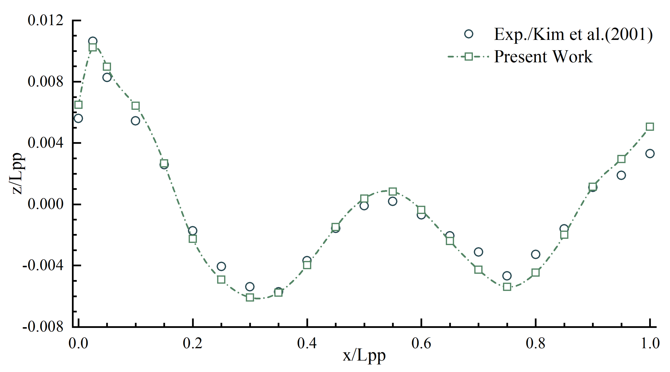
Figure 8 presents comparisons of the wave heights on the hull surface at Fr = 0.260. It can be seen from Figure 8 that the single-step method could also track the trend of waves on the hull precisely, especially the locations of crests and troughs, which were in good agreement with test values. Overall, the predicted wave crests at the bow and midship fitted better with the measurements, while the wave height of troughs near the midship was lower than that of the tests, and the errors were relative larger compared with the other positions.

As a result, the VOF single-step method was able to track and simulate the wave characteristics of the KCS hull. The reliability and effectiveness of this method for modeling the flow field were verified and validated.

4.3. Resistance Prediction and Flow Field Analysis

Compared to the single-step method, the VOF Multi-step method introduces time sub-cycles into the volume fraction transport equation, which can significantly improve the resolution of the two-phase fluid flow interface and capture the shape of the free surface effectively. The number of inner iterations in user-defined implicit multi-stepping permits a time step size N times greater than single-stepping. The solution time for the inner iterations is much lower than that required to shorten the time step, thus significantly reducing the cost with guaranteed result accuracy.

4.3.1. Computational Cost

This section compares the resistance prediction results and flow field characteristics of implicit multi-stepping with single-stepping. Based on the N₂ grid configuration, the time steps Δt₁ and Δt₂ were chosen for the single-step method in the CFD simulations. The implicit multi-step method, based on Δt₂, calculated the calm water resistance and flow field for inner iteration numbers of 1, 2, and 4, where the number of inner iterations is the number of iterations performed in a loop.

Table 6. Comparison of motion and resistance coefficients of different VOF methods.

Case	Method	Resistance Coefficient	Error	Trim (deg)	Sinkage (m)
case 1	SS_0.01 s	0.0036944	0.447	−0.1716800	−0.01359466
case 2	SS_0.005 s	0.0036809	0.812	−0.1694570	−0.01366240
case 3	IM(1)_0.01 s	0.0036944	0.447	−0.1716700	−0.01366019
case 4	IM(2)_0.01 s	0.0036780	0.890	−0.1730820	−0.01367844
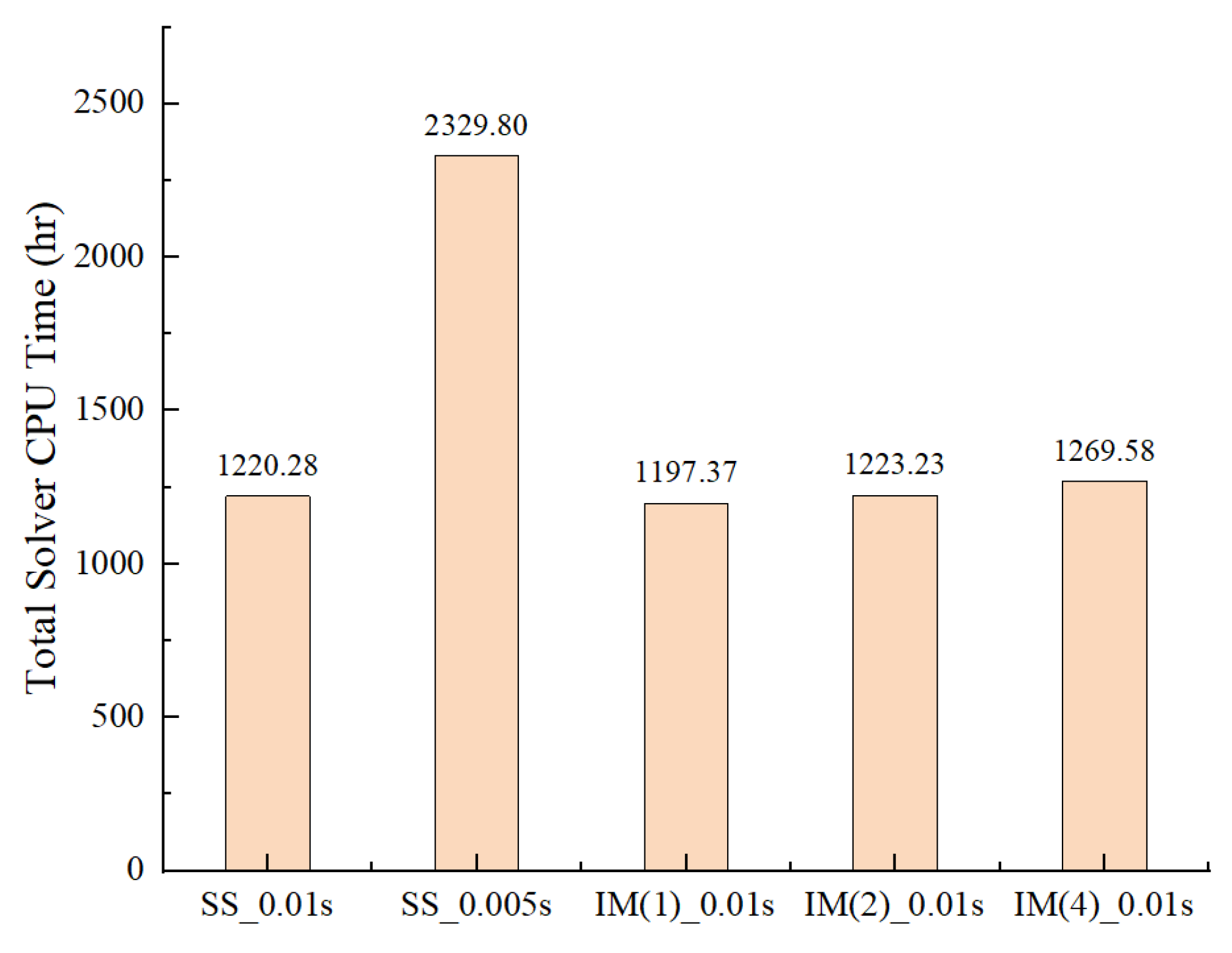
case 5	IM(4)_0.01 s	0.0036784	0.880	−0.1727190	−0.01366914

and Figure 9 illustrate the results of the ship resistance calculation using different VOF methods and a comparison of the computational costs, where case 1 is a single-step method with a time step of 0.01 s; case 2 is a single-step method with a time step of 0.005 s; and cases 3, 4, and 5 are implicit multi-step methods with internal iterations of 1, 2, and 4, respectively, and all with a time step of 0.01 s.

As shown in Table 6, it can be seen that the results and solution time were almost the same for the single-step method (case 1) and the implicit multi-step method with the iteration number taken as one (case 3) for the same time-step size. Both were able to accurately resolve the ship resistance and attitude of the KCS with an error of less than 0.5%. Cutting the step size to half that of case 1 (case 2), the VOF single-step method could predict the main parameters precisely with an error of −0.27% in trim, but the computational cost required was 1.91 times that of case 1.

The implicit multi-step approach resolved the volume fraction N times in each flow time step to obtain a clear interface. The resistance and heave results for both agreed well, with a maximum error within 0.15%. For trim calculations, the VOF implicit multi-step method (case 4 and case 5) provided relatively large errors of −2.201% and −2.415%, yet the costs were only 0.53 and 0.55 times that of single-stepping (case 3), reducing the solution time for predictions significantly.

4.3.2. Free Surface

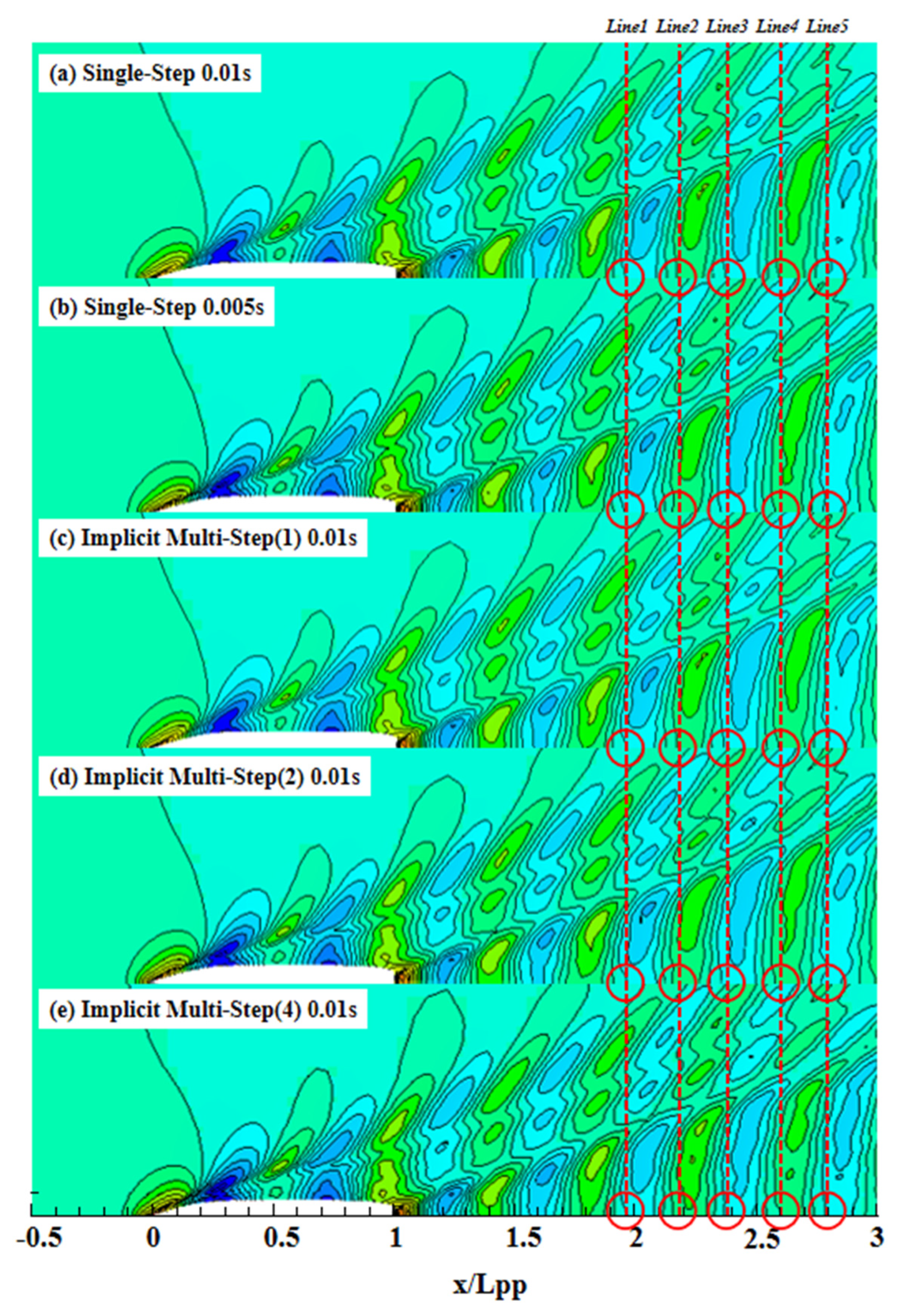
Figure 10 shows a comparison of the flow field distribution between the VOF single-step method and the implicit multi-step method for solving the free surface waves. The results demonstrate that both methods could simulate the wave features of the KCS model, and no obvious wave dissipation phenomenon is observed in the far field. In the case of waves near the hull, the implicit multi-step approach could trace the location of wave crests and troughs, and the wavelengths corresponded well to the experimental values. The above flow field predictions were consistent with single-stepping.

The wavelengths of free surface waves in the far field region exhibited small differences. Lines 1–5 indicate the location of the wave height contours at different distances from the stern (case 1). Line 1 was located about one time the ship length to stern, and the predicted wave heights in cases 1–5 were in good agreement with Line 1. Lines 2–5 were placed in the far field, where the simulated wave locations of cases 2–5 were ahead of those of case 1 and closer to the experiments. The shapes of free surface waves in case 1 and case 3 were generally consistent, with wavelengths slightly lower than the calculations in the single-step method. With the implicit multi-step approach, when the number of inner iterations was 2, the results were similar to those obtained by reducing the time-step size to half that of the original. The wavelength and shape of waves in far field region matched well. Increasing the number of inner iterations to four, the wavelength in the far field was similar to that in case 2 and case 4, but the shape of the waves was quite different from both, especially in the region after Line 5 (see Figure 10e).

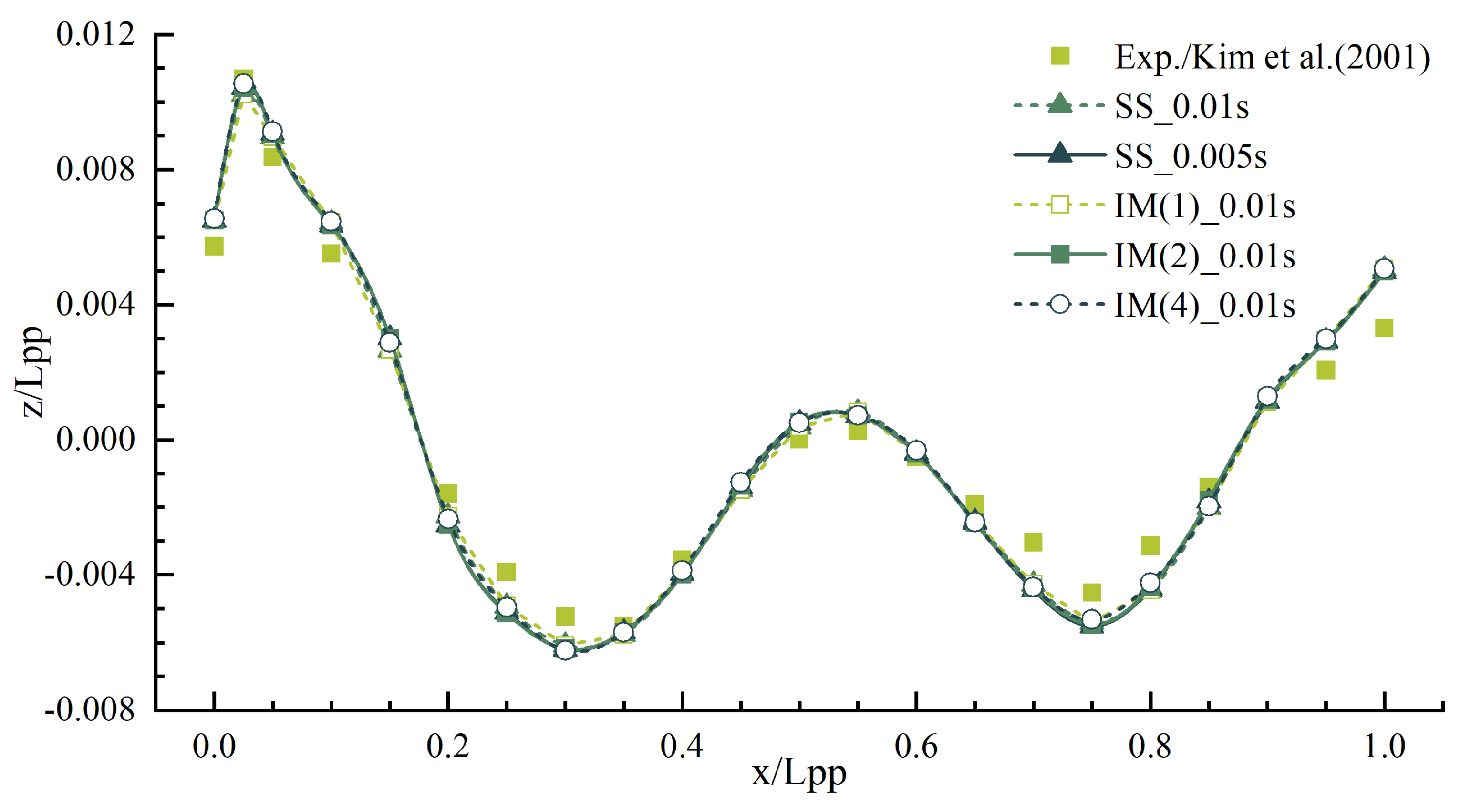
As can be seen from Figure 11, the VOF implicit multi-step method can simulate the trend of the hull surface waves more accurately. Compared to the experiments, our method provided a more accurate result for the location and height of wave crests at the bow and midship, while it was relatively incorrect for waves near the midship trough and at the stern. At the same step size, the single-step (case 1) and the implicit multi-step approaches (case 3) with an inner iteration number of one provided similar results, except the latter were closer to the tests. The numerical calculations for the implicit multi-step method with two inner iterations (case 4) agreed well with the results of case 2. Increasing the number of inner iterations to four (case 5), the calculations for the trough near the midship were closer to the measurements and corresponded closely with the actual trend of the waves on the hull surface.

In comparison to single-stepping, the implicit multi-step approach has significance with respect to capturing the location and shape of the two-phase fluid flow interface with reducing solution time. The following introduces a comparison between the single-step and implicit multi-step methods, with the pressure and wave distribution near the bow.

According to Figure 12, the VOF implicit multi-step approach was equivalent to the traditional single-step method, when the number of inner iterations was taken as one. The surface pressure distribution at the bow was generally consistent. The results for the inner iteration number of two were in good agreement with the case of reducing the step size (case 2).

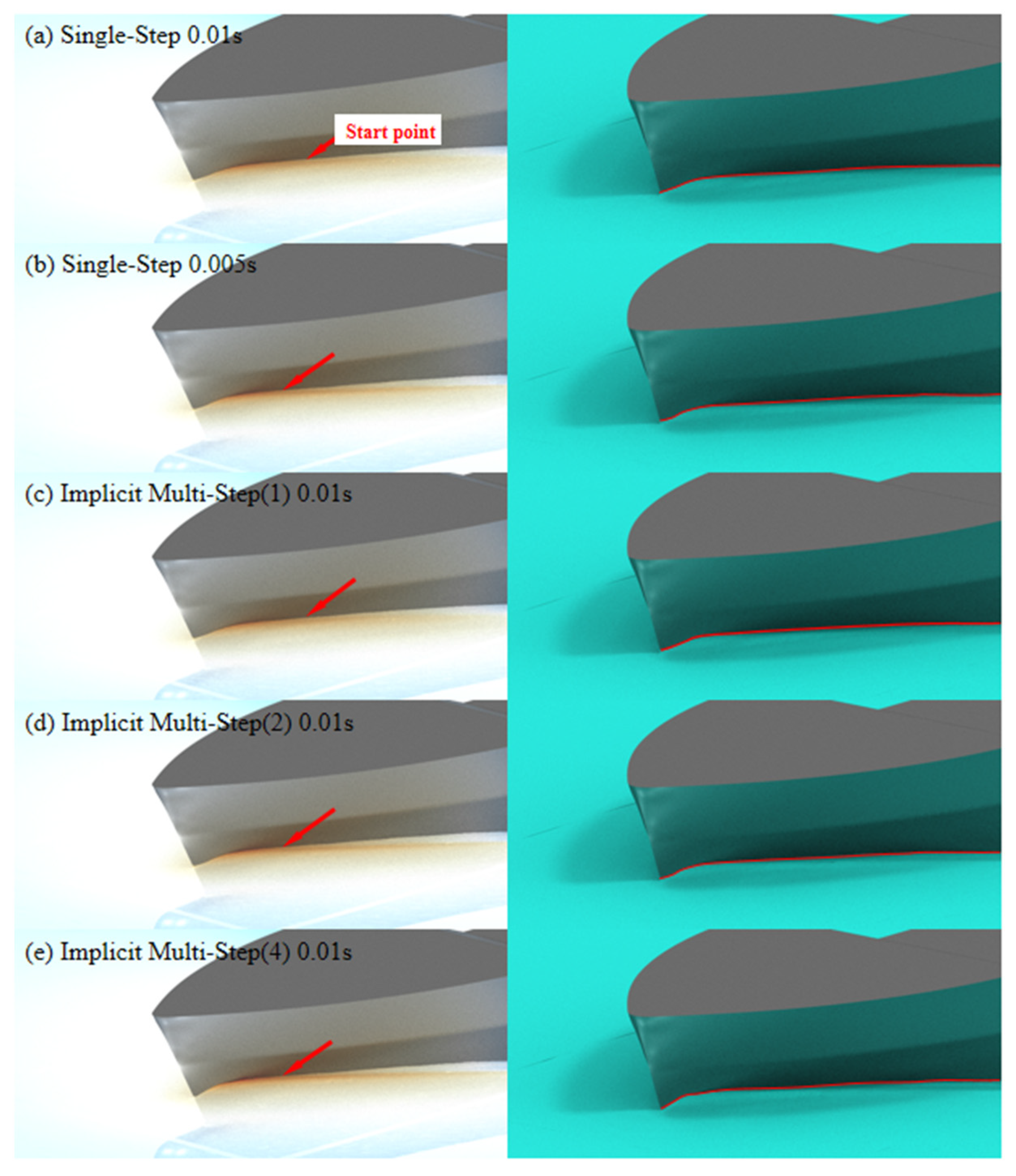
Figure 13 shows a comparison of simulations of the shape of bow waves using the different models. As can be seen from the right column of Figure 13, the implicit multi-step method with an internal iteration number of one agrees well with the waveform model in case 1. As the number of internal iterations is increased to two, the trend of the bow wave based on the implicit multi-step method is the same as in case 1 and case 3. Increasing the number of internal iterations to four, the shape of the waves becomes closer to the bow. The trend of the hull surface wave also matches well, but the decline after the first wave peak is relatively slow. As can be seen in the left column of Figure 13, the implicit multi-step method with an internal iteration number of one agrees with the predictions of case 1 in terms of the trend of the hull surface wave and the onset of the ship’s wave decline. As the number of internal iterations is increased to two, the location of the start of the wave’s descent is closer to the bow of the ship. Increasing the number of internal iterations to four, the location of the wave descent point agrees with cases 2 and 4.

5. Conclusions

In this paper, calm water resistance simulations for a standard KCS model at Fr = 0.260 were performed based on CFD method. The calculation results and flow field of both the single-step and multi-step methods were compared and analyzed, and then, we discussed the strengths and limitations.

The calculation results of the model using an implicit multi-step method with reasonable internal iterations were close to those using a single-step method with a reduced time step method. At the same time-step size, the single-step and the implicit multi-step approaches with an inner iteration number of one provided similar results, and the solution time required was the same, with an error within 0.5%. As the inner iterations increased to two, the multi-step method and single-step method with reducing step size had a better fit in terms of resistance and heave, while the error in trim was greater than single-stepping. The error for both was about 2%, while the solution time was only 0.53 times that of the latter. Increasing the inner iteration number to four, the error in the predicted trim values of multi-stepping was relatively low, and the solution time was only 0.55 times that of single-stepping.

Compared to the single-step approach, the implicit multi-step method had significant advantages in capturing the position and shape of the free surface at a lower time cost. When the number of internal iterations was sufficient, the implicit multi-step method could accurately capture the pressure distribution near the bow, and the shape and position of the bow wave. However, in the far field range (2.0–3.0 L) the wavelengths predicted using the multi-step method were closer to the experiments, but the shapes of the waves differed from the experimental measurements for a larger number of inner iterations.

This work only verified the feasibility of the VOF implicit multi-step method for ship hydrodynamic prediction, excluding ship self-propulsion and maneuvering. Future research will discuss whether the VOF implicit multi-step method can be applied to ship self-propulsion and maneuvering [29], and deeply investigate and verify the effect of the number of inner iterations on ship hydrodynamic calculations.