Article

A Simplified Approach for Predicting Bend Radius in HDPE Pipelines during Offshore Installation

1
McDermott Asia Pacific, Kuala Lumpur 50250, Malaysia
2
Department of Civil and Environmental Engineering, Universiti Teknologi PETRONAS, Seri Iskandar 32610, Perak, Malaysia
3
Ocean and Shore Technology (OST) Research Group, Department of Naval Architecture and Ocean Engineering, Seoul National University, Seoul 08826, Republic of Korea
4
School of Civil, Environmental and Architectural Engineering, Korea University, Seoul 02841, Republic of Korea
5
Research Institute of Marine Systems Engineering, Seoul National University, Seoul 08826, Republic of Korea
*
Authors to whom correspondence should be addressed.
J. Mar. Sci. Eng. 2023, 11(10), 2032; https://doi.org/10.3390/jmse11102032
Submission received: 9 September 2023 / Revised: 11 October 2023 / Accepted: 13 October 2023 / Published: 23 October 2023
(This article belongs to the Section Ocean Engineering)

Abstract

:
Traditionally, subsea pipelines designed for the transportation of oil, gas, and water are constructed using carbon steel due to its strength, toughness, and ability to operate at temperatures up to 427 °C. However, polyethylene (PE), especially its high-density variant (HDPE), presents advantages such as reduced installation costs, diminished water leakage, and superior corrosion resistance. As research endeavours to enhance PE properties, its adoption for subsea applications is anticipated to rise. This study first delineates the mechanical behaviour of HDPE pipelines for offshore installation, identifying pulling tension, dimension ratio, water depth, and air fill ratio as the paramount lay parameters. Subsequently, a theoretical bend radius equation was derived from pipelaying mechanics using a purely geometric approach. Within this equation, two determinants, parameter X and parameter Y, dictate the sagbend bend radius. Regression analysis elucidated the relationships of lay parameters with both X and Y, yielding a general equation for X in terms of pull tension, water depth, and air fill ratio and another for Y as a function of water depth. Together, these geometric determinants underpin the sagbend bend radius estimation model. For overbend bend radius prediction, a lay index (IL) was fashioned from the aforementioned three parameters. Correlation assessments between the lay index and overbend bend radius revealed R2 values of 0.940, 0.836, and 0.712 for pipes with diameters of 2.0, 2.5, and 3.0 metres, respectively. This underscores the model’s proficiency in predicting the bend radius, albeit with decreasing precision for larger-diameter pipelines.

1. Introduction

In recent times, non-metallic pipes have gained precedence in offshore project development. A multitude of research has delved into understanding the behaviour of such pipelines [1,2,3]. High-density polyethylene (HDPE) often finds use as an internal lining for steel pipes in marine environments and forms part of composite pipe material. Regarding the HDPE, limited studies have been conducted recently, as follows.
Kuliczkowska and Gierczak [4] examined the buckling failure mechanisms of HDPE rehabilitation pipes and assessed various design strategies against this issue. Their research revealed notable discrepancies in different calculation methods and highlighted key factors in buckling evaluation. Yang et al. [5] investigated the abnormal leakage effect of a buried HDPE pipe. They concluded that most of the failures may be caused by erosion–corrosion and mechanical damage and have investigated the biological degradation. Wu et al. [6] conducted field explosion tests on buried HDPE pipelines, analysing factors influencing dynamic responses. Based on their findings, they established explosive charge standards and devised damage prediction models for different damage levels. Majid and Elghorba [7] conducted HDPE pipe failure analysis by a static test and proposed simplified approaches to assess the damage. Guidara et al. [8] performed a structural integrity assessment of defected HPDE pipes. They focused on the burst test and FE-based ECA by a J-integral technique. Guidara et al. [9] continuously proposed a semi-empirical model for structural integrity assessment for HDPE pipes. However, studies related to subsea pipeline installation using HDPE pipes are limited.
Other frequent linings include polyvinyl chloride (PVC), fusion-bonded epoxy (FBE), and corrosion-resistant alloy (CRA) [10,11]. Conversely, pure HDPE pipes dominate the construction of seawater intake and discharge systems in coastal processing facilities. Extensive research has been conducted on the installation of offshore carbon steel pipelines and pipe-in-pipe systems [12,13,14]. However, offshore HDPE pipeline installations diverge from carbon steel installations, primarily because of HDPE’s lightweight properties. Carbon steel pipes predominantly employ the S-lay and J-lay installation methods. The S-lay process sees the pipeline transition from a horizontal vessel position, curving downwards to the seabed in an emblematic S-shape. In contrast, the J-lay method, preferred for deeper waters, deploys the pipeline from a vertical lay system (VLS) tower, assuming a J-shape [15].
Pipelines during offshore installations endure external pressure, bending, and axial load from various environmental forces [16,17], impacting their fatigue life over operational phases [18,19,20,21]. Hence, ensuring pipelines perform as designed without compromising integrity is paramount. Analytical optimization of the design is vital for effective real-world operation, underlining the importance of a profound understanding of installation analysis modelling techniques. HDPE pipes in marine applications, predominantly for water intake or discharge, are favoured due to their high corrosion resistance, low surface roughness (enhancing hydraulic behaviour), and exceptional resilience against environmental forces. Roberts et al. [22] indicated that outfall diffuser depths typically range from 20 m to 40 m. Pipelines situated in water depths beyond 60 m are classified as deep water. Notably, in 2012, Makai Ocean Engineering undertook a repair study on a 40” diameter HDPE intake pipeline located at a depth of 670 m. Utilising the Orcaflex software (ver 9.6), Rocheleau and Jensen [23] crafted a finite element (FE) model to emulate a large-diameter catenary HDPE pipeline and its anchoring system, enhancing the repair methodologies through a better understanding of design behaviour.
Several authors, including Johansen et al. [24] and Ravlic et al. [25], have illuminated the challenges of subsea pipeline installations. In brief, the challenges including the research gap and the technical reviews on HDPE pipeline studies and guidelines are concisely illustrated in Figure 1a,b. More recently, Kim et al. [26] detailed the design and installation of an ultra-large HDPE intake pipeline in Algeria, boasting a diameter of 2.5 m and dimension ratios of 26 and 30. The pipe dimension ratio (DR) is defined as the ratio of a pipe’s outer diameter to its wall thickness. Intriguingly, as the DR increases, indicating a larger diameter, the wall thickness proportionally decreases.
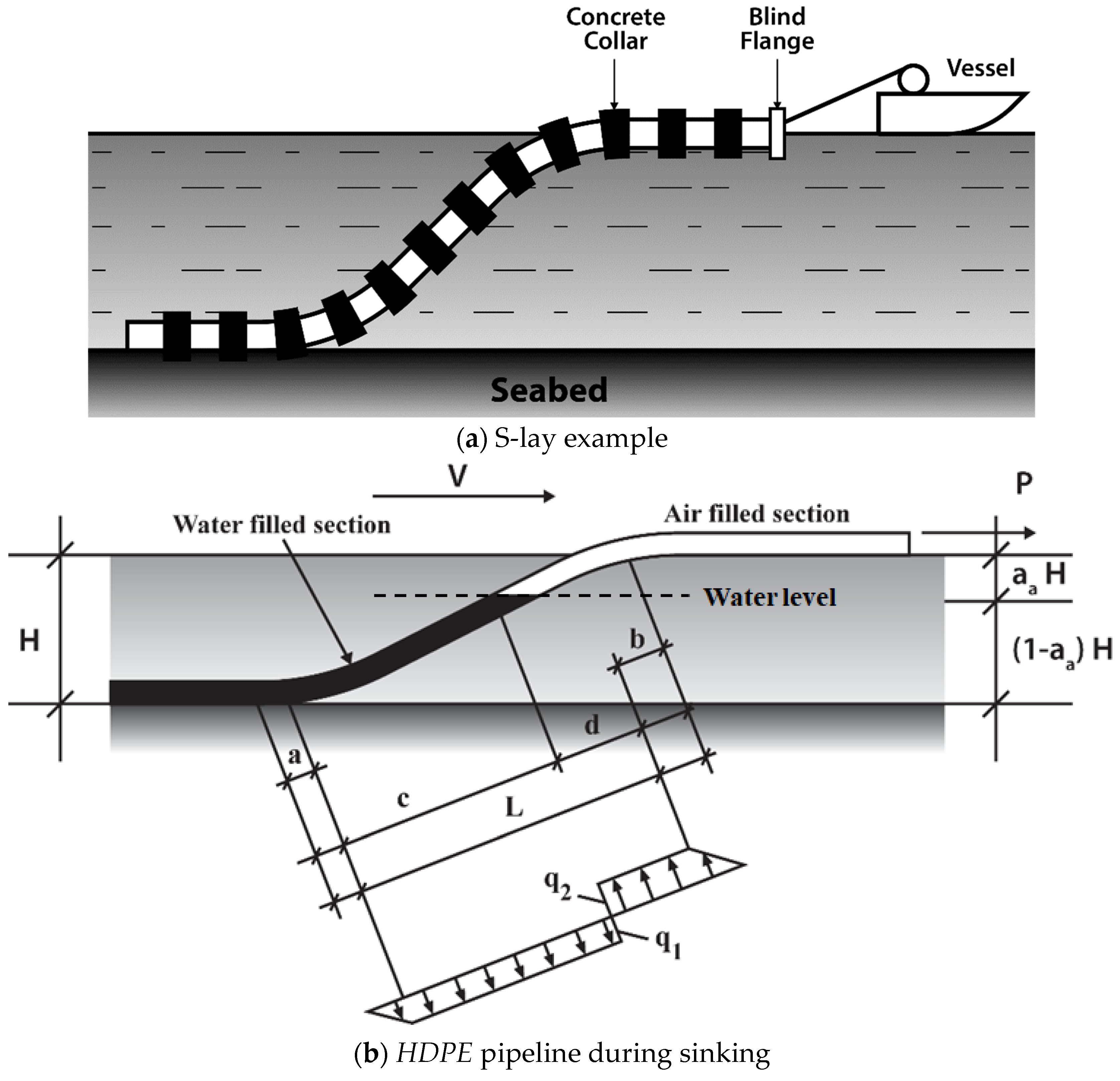
A critical observation was that the pipe’s simplified minimum yield stress (SMYS) stood at a significant 92%, especially when considering a 70 kN pulling force. The HDPE pipeline is typically installed via the float-and-sink method, as illustrated in Figure 2a. Enhanced modelling techniques during the sinking phase can potentially yield improved analysis results. Since the introduction of PE pipes for marine installations in the late 1950s, the S-lay sinking method has predominantly been employed. As presented by Andtbacka et al. [33], the essential premise of this method involves the pipe initially floating on the seawater’s surface, followed by water being filled from one end while pull tension is exerted at the opposite end.
However, a novel conceptual study by Stentiford and Wooley [27] proposed three distinct installation methods for PE pipelines for depths of up to 1000 m. The first, known as the ocean surface floating tow method, requires buoyancy modules to be fixed at specific intervals. These modules ensure the pipeline’s top breaches the seawater’s surface. Following this, the pipeline is towed to its designated location by a tugboat. Once in position, buoys are gradually released, causing the pipeline to descend onto the seabed. The second method, termed the buoyant catenary, employs a clump weight attached at both the inshore and offshore ends of the pipeline. Installation is orchestrated so that both weights descend to their respective positions. Due to its low-density nature, the buoyancy of the PE pipeline makes it assume an inverted catenary shape. Lastly, the ocean floor tow method allows the pipeline to be towed out to sea, hovering just above the seabed to minimise current impacts.
Historically, the definition of “large diameter” for PE pipes has evolved. In 1982, a pipe with a 1.0 m diameter and a dimension ratio of 23 was deemed large [28]. By 2009, marine cooling water pipelines for the Terga power plant were being constructed with a diameter of 2.0 m and a dimension ratio of 26 [34]. Presently, PE pipes are manufactured in sizes reaching up to 3260 mm in diameter, with dimension ratios ranging from 17 to 41 [35]. Consequently, it is plausible to infer that mechanical properties consistent with pipes smaller than 3.0 m can be achieved, given the similarity in dimension ratios. This research endeavours to provide insights into the characteristics and behaviour of large-diameter HDPE and to introduce a streamlined model to predict the bend radius of the pipeline during offshore installation. This study specifically examines pipes of 2.0 m, 2.5 m, and 3.0 m in diameter, spanning dimension ratios of 17, 21, 26, 33, and 41.

2. Sinking Process Mechanism

Earlier research primarily relied on static analysis of pipeline issues. Initially, the pipeline profile, often assumed to adopt an S-shape during the sinking operation, was an unknown variable. The most critical stage is the sinking process, depicted in Figure 2b. For a successful installation, it is imperative to strike a balance between the downward forces (q1) and upward forces (q2). Downward forces primarily stem from the concrete weights attached to the pipeline, while the buoyancy of the air-filled pipeline section generates the upward forces.
For the sinking process to commence and progress, the downward forces must slightly outweigh the upward forces. However, maintaining this delicate balance remains a central challenge. It is crucial to prevent the acceleration of downward forces; this can be managed by monitoring the sinking speed and adjusting the internal air pressure accordingly. If sinking speed escalates, air pressure can be increased, and the reverse is also true. Tools like valves and compressors play a vital role in regulating this pressure. A primary concern for the pipeline is potential damage due to buckling at the sea’s surface or bottom, caused by bending. As illustrated in Figure 2b, key factors influencing the sinking process include upward and downward forces, pulling force (P), air pressure, and sinking velocity (V). Notably, this study specifically focuses on the upward, downward, and pulling forces.

3. Study of Interest

To develop a simplified method for predicting the bend radius of large-diameter HDPE pipelines, we delved into the following research domains:
  • Analysing the impact of depth variation on the pipeline’s total stress and curvature.
  • Investigating the influence of applied tension variations on total stress and curvature.
  • Evaluating the effect of the pipe’s dimension ratio (DR) on total stress and curvature.
  • Comparing results for pipe diameters of 2.0 m, 2.5 m, and 3.0 m.
  • Conducting a regression analysis on the primary parameters for pipeline installation.
  • This study presents analysis results obtained from static modelling. In this initial study, static analysis is adequate to obtain the effect of water depth, pull tension, pipe DR and AFR on pipe curvature or bend radius for the formulation of bend radius prediction. Hence, dynamic analysis, which takes into account the vessel and pipeline hydrodynamic behaviour, has not been analysed.

3.1. Sinking Model

This research explored various modelling techniques to simulate the structural response of HDPE pipeline sinking operations, as depicted in Figure 3 and Figure 4. The pros and cons of each sinking method are detailed in Table 1 and Table 2. Three modelling techniques were compared to assess the stress load distribution on the pipeline. The decision matrix method facilitated the identification of the most suitable technique among the three, considering criteria such as load distribution, model complexity, and sagbend and overbend stress ratios. Load distribution pertains to the load imposed on the pipe due to arbitrary buoys, clumps, or weights in the model, with techniques A and B demonstrating high values. Model complexity reflects the intricacy of each technique, gauged by the number of objects involved. The stress ratio gauges the analysis loading stress against the PE’s minimum yield strength in the sagbend and overbend regions. Preliminary findings identified the equivalent weight method as the superior approach for modelling HDPE pipeline sinking (see Table 3). Consequently, Model C, representing this method, was chosen for the parametric study analysis.

3.2. Effect of Depth Variation

For this investigation, the finite element software OrcaFlex (version 9.6) was chosen to analyse the impact of various parameters on the resulting stresses and strains. The properties of the pipe utilised in this study are detailed in Table 4, Table 5 and Table 6. An initial pull tension of 153 kN, calculated using Equation (1), was applied to assess the influence of varying depth values on the pipelay’s shape, as well as its stress and strain responses.
T = w s u b × w . d .
Here, T is the tension (kN), w s u b is the pipeline’s submerged weight, and w . d . (mm) is water depth.
Table 4. Pipe data.
Table 4. Pipe data.
DescriptionUnitPipe
Outer diametermm2000
Wall thicknessmm77
Table 5. Material data.
PropertyUnitValue
Densitykg/m3960
Yield strengthMPa23
Tensile modulus (short)MPa950
Poisson’s ratio-0.4
Minimum required strength (MRS) MPa10
Table 6. Concrete collar data.
DescriptionUnitValue
Spanm6
Air fill rate%20
While maintaining a constant tension, the water depth was varied in increments of 10 m to observe its effects on the pipeline until it reached a point of overstress or buckling. As observed, with an increase in water depth, the pipeline profile tends to become steeper. Figure 5 and Figure 6 illustrate the stress and curvature variations in the pipeline throughout the sinking process. Notably, as the water depth rises, there is a corresponding increase in both stress and curvature when tension remains unchanged. It is crucial to highlight that, depending on the chosen design criteria for installation, the results can vary significantly. For instance, under stress limit criteria, the pipeline can sustain depths up to 27 m before failure, as depicted in Figure 5. In contrast, if considering the local buckling limit, this threshold extends up to 60 m before observing a failure.
w . d . = 12 O D
In line with Pipelife’s guidelines, water depths greater than 24 m qualify as the “deepwater” region, as formulated in Equation (2) [36]. Due to the unique challenges and conditions present in deepwater installations, the pulling tension needs to be adapted. To accommodate for these depths, the pull tension was adjusted to double its previous value, increasing it to 300 kN. This study further examined increasing water depths, beginning from a 30 m depth and incremented in 20 m intervals. The results of this approach, including the impact on stress, curvature, and any observed buckling or failure points, are discussed in the subsequent sections.
In evaluating the stress design parameters, it was discerned that the pipeline reached an overstressed condition at a relatively shallow depth of 27 m. When the pulling tension was strategically augmented to account for challenges inherent to deepwater operations, there was a modest reduction in pipeline stress, bringing it down to 14.3 MPa. Yet, upon incrementally increasing the water depth, the pipeline swiftly approached its stress threshold again at a depth of 30 m, a phenomenon illustrated in Figure 7. Parallel observations made on pipe curvature, as demonstrated in Figure 8, offer insight into its behaviour across a spectrum of water depths, ranging from 30 m up to a critical point where buckling transpired at 90 m. A pivotal observation from this analysis is the predominant influence of pulling tension adjustments on the pipeline’s curvature (or bend radius) in contrast to the impact it has on the pipeline stress.

3.3. Effect of Tension Variation

The integrity and profile of a pipeline are significantly influenced by the pulling tension applied. To delve deeper into the effects of varying tension parameters, we systematically increased the pull tension in increments of 150 kN, culminating at 450 kN. Figure 9 vividly captures the subsequent transformations in the sagbend curvature as the tension escalates.
The repercussions of heightened pulling on the pipeline’s stress and curvature dynamics are comprehensively depicted in Figure 10 and Figure 11. Notably, escalating the pull tension results in a marked decline in the maximum stress and curvature, both in the overbend and sagbend zones. However, this diminishing effect is considerably more pronounced in the sagbend region compared to its counterpart. To quantify, tension enhancement from 153 kN to 450 kN triggers a 13.5% reduction in curvature in the overbend zone, while the sagbend region experiences a more substantial drop of 26.7%, as corroborated by Table 7.

3.4. Effect of Pipe Dimension Ratio

The pipe’s dimension ratio (DR) is defined as the ratio of a pipe’s outer diameter to its wall thickness. Intriguingly, as the DR increases, indicating a thicker diameter, the wall thickness proportionally decreases. For the scope of this analysis, our reference pipeline spotlights a DR of 26. This section critically assesses the ramifications of varying pipe DRs on integral aspects of the pipe—notably its stress and curvature. A deliberate selection of five DR values, which are prominently utilised in manufacturing, forms the foundation of this study. These chosen DRs are 17, 21, 26, 33, and 41. In our numerical simulation, a pipe with a 2.0 m diameter saw its wall thickness methodically reduced across the specified DRs: from 117 mm, progressing to 95 mm, 77 mm, 60 mm, and finally reaching 49 mm.
The profound influence of DR on the bend radius, specifically in the sagbend and overbend regions, is meticulously explored. Figure 12 and Figure 13 encapsulate the tangible effects of stress and curvature on the pipeline across the spectrum of the five DR variations. Of these, the pipe with a DR of 41 manifested the most pronounced stresses and curvatures. In stark contrast, the pipe characterised by a DR of 17 showcased the least stress and curvature. Synthesising these observations, it is discernible that a pipe with a lower DR is advantageous. Not only does it boast a more expansive cross-sectional area conducive to stress mitigation, but its robustness also empowers it with enhanced resistance to bending loads.

3.5. Effect of Pipe Diameter

The focal point of this study is on large-diameter, high-density polyethylene (HDPE) pipes. An essential parameter under investigation is the interplay between the pipe diameter and its consequential effects on both pipe stress and curvature. Throughout this exploration, the pipe’s dimension ratio (DR) was held constant at a value of 26. A comprehensive analysis was executed on pipes with diameters spanning 2.0 m, 2.5 m, and 3.0 m. As depicted in Figure 14, intriguingly, the diameter does not exert a pronounced influence on the pipeline stress, particularly in the overbend region. The stress variations here are negligible, illustrating a near-uniform stress distribution irrespective of the diameter. Conversely, in the sagbend region, a marginal escalation in stress is discernible with increasing diameter.
Figure 15 provides a more nuanced understanding of the curvature dynamics. There is a marked amplification in pipe curvature, evident in both the overbend and sagbend regions, directly attributable to diameter augmentation. This observation underscores the criticality of meticulous design considerations for large-diameter pipelines. Their heightened susceptibility to local buckling, especially under bending loads, mandates rigorous design and evaluation protocols.

3.6. Effect of Pipe Air Fill Ratio (AFR)

As indicated in Figure 16, the float-and-sink profile of a floating HDPE pipeline varies with the air fill ratio (AFR) property, a widely recognised parameter in the industry to characterise the loading degree during the sinking phase. The AFR represents the fraction of the internal volume of the pipe that must be air-filled to achieve balance with the ballast weights attached [22]. Additionally, AFR correlates with the water level elevation inside the HDPE pipeline beneath the sea surface, as illustrated in Figure 2.
Analysis of a 2.0 m diameter pipe submerged at a 30 m water depth with a tension of 200 kN showcased the influence of AFR on the pipe’s peak stress and bend radius, as depicted in Figure 17 and Figure 18. Notably, the maximal stress is minimised at an AFR of 10% and escalates to its peak within the 30–35% AFR spectrum. Beyond an AFR of 40%, its influence on pipe stress becomes negligible. In terms of both structural integrity and cost efficiency, a lower AFR is preferable.
Furthermore, the bend radius’s relationship with AFR is evident in Figure 18, indicating a reduction in the bend radius as the AFR climbs. This reduction effect is particularly pronounced in the sagbend region compared to the overbend. A decreased AFR facilitates the use of lighter ballast weights on the pipeline, ensuring the stability of the anchored pipeline remains paramount. Employed weights must sufficiently anchor the pipeline, guaranteeing vertical and horizontal stability, be it within a trench or directly on the seabed [29].

4. Geometric Formulation of S-Lay Bend Radius

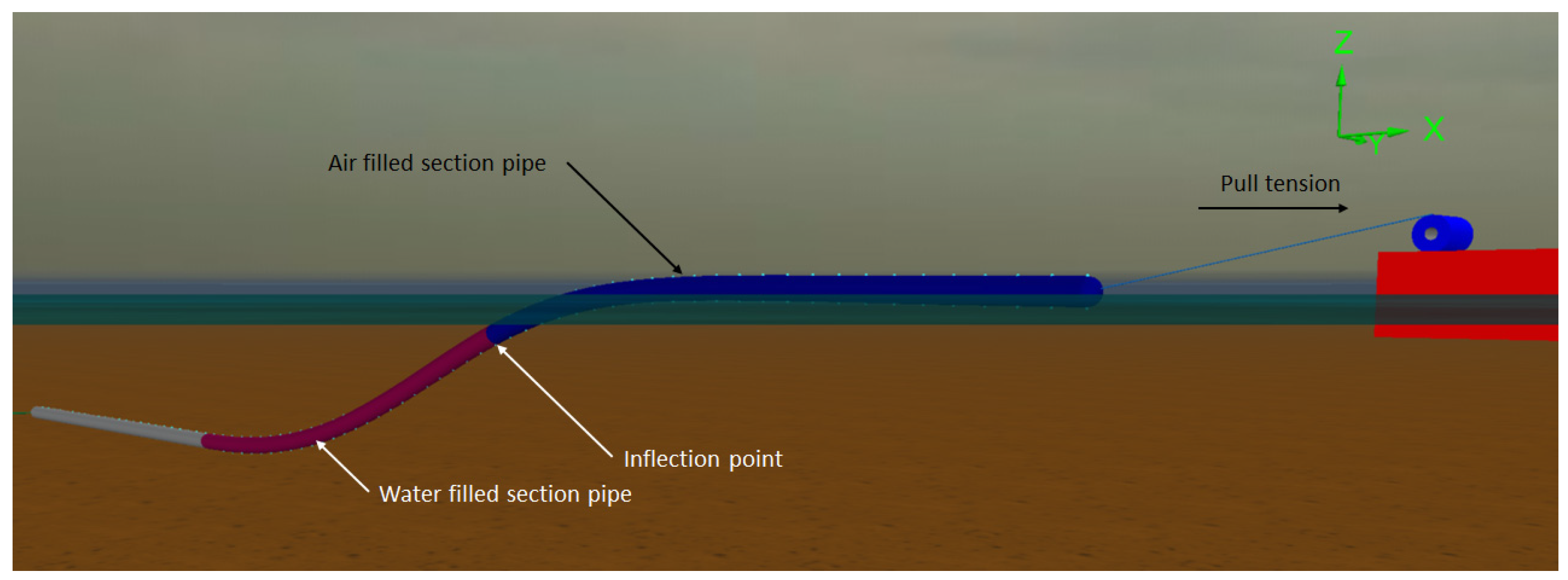
During the float-and-sink operation, the pipeline’s static configuration is primarily influenced by two factors: the pulling tension and the internal air pressure. Of these, only the pulling tension can be actively controlled during the sinking process, given that the bend radius inherently depends on this tension. This axial tension in the pipeline is characterised by both vertical and horizontal components.
The vertical component arises from the combination of the water depth and the weight of the flooded pipe. In contrast, the horizontal pull tension serves a crucial role in managing the characteristic “S” configuration of the pipeline as it transitions from the water’s surface to the seabed. This transition can be segmented geometrically into two distinct sections: the overbend and sagbend, visualised in Figure 19. From the configuration provided in Figure 19, a relationship between R, X, and Y is derived, with the Pythagoras theorem offering the foundational basis for the relationship, as articulated in Equation (3):
R = X 2 + Y 2 2 Y
where R represents the pipe’s bending radius in the sagbend region. The parameter X denotes the horizontal distance between the inflexion point and the touchdown point (TDP), while Y signifies the vertical distance from the inflexion point to the seabed. Additionally, “w.d.” refers to the water depth, and AFR stands for the air fill ratio. Interestingly, a design with a 50% air fill ratio results in comparable pipe curvature in both the overbend and sagbend regions.
In practical scenarios, the general understanding is that the bend radius along a catenary continuously decreases, reaching its minimum value in the touchdown zone (TDZ). However, this study’s focus is on large-diameter pipes, characterised by their heightened bending stiffness. As a result, the influence of the bend radius on the catenary’s shape becomes less pronounced.

5. Identification of Parameters X and Y

The geometry of parameter (Xh) also depends on the water depth, tension, and AFR [29]. The general equation derived for this parameter is:
X h = K ( T 200 ) + X i
K = 6 D 2 + ( 14 w . d . ) D + 4 w . d . + 7 5000
In the equation, the factor “K” stands as the slope of the regression line when comparing tension to the parameter—Xh. This slope, represented by factor K, conveys the rate of change in parameter X with respect to the pull tension, T. Furthermore, the term Xi designates the initial horizontal distance. Given that both the water depth and the pipe diameter influence the parameter X, the factor K is adjusted to encompass effects from these variables, making it a function of both water depth and pipe diameter.
To shed light on this relationship, a correlation analysis was conducted. This analysis assessed the water depth—acting as the predictor—across all three pipe sizes in relation to factor “K”. Figure 20 captures this relationship, showcasing a positive linear regression for pipes with diameters of 2.0 m, 2.5 m, and 3.0 m. Stemming from these observed relationships, a more comprehensive equation, Equation (5), was crafted. This equation positions factor K as a function of water depth and pipe diameter, and it is grounded in the principles of linear regression analysis.
Since Xi is the initial horizontal distance (pipeline without pull tension), it is dependent on the water depth and AFR property. Figure 21 shows that X i and A F R have a power relationship with constants A and n as Equation (6). This diagram also demonstrates that these constants are dependent on water depth. As water depth increases, the constant A and n increase as well. Hence, the correlation of constant A and n as a function of water depth and pipe diameter was established. From a simple correlation study, both constants A and n have quadratic correlation, and the general equation for these constants can be derived as shown in Equations (7) and (8).
X i = A A F R n
A = 0.005 w . d . 2 + 0.7 w . d . + 5 D + 12
n = 0.00005 w . d . 2 0.0004 w . d . + 0.4 + 0.015 D
Thus, combining all of these functions, the general equation for parameter X h is proposed as below:
X h = 6 D 2 + ( 14 + w . d . ) D + 4 w . d . + 7 5000 T 200 + A A F R n
Factor = water   depth constant   term
Y v = w . d . 4 A F R + w . d . 2.86
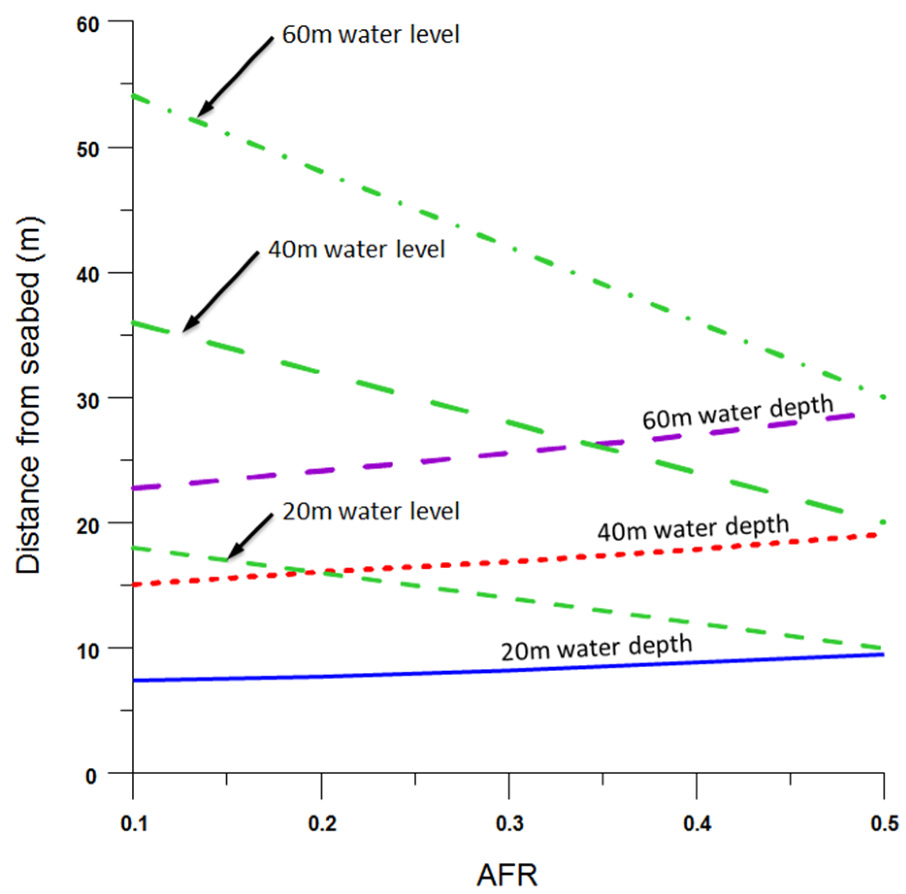
The relationship developed between AFR and Y is a linear regression line with linear term m and constant term C. Constant (m) is the slope, and (C) is the y-intercept where both of these values are functions of water depth. Based on the parameter Y v profile in Figure 22, there is a positive linear correlation observed between (m) and (C) and the water depth. As water depth increases, these two constant terms increase as well. Thus, from observation, factors (m) and (C) can be obtained from Equation (10). Table 8 summarises this correlation and the recommended factor values. The recommended values were selected by averaging the factor for each water depth linear profile. Then, these two-factor values were substituted into a linear equation to form a general equation for estimating the inflexion point location or lay vertical parameter Y. Hence, the recommended general equation derived for parameter Y v proposed is as Equation (11).

6. Simplified Bend Radius Prediction Method

6.1. Sagbend Bend Radius

The previously discussed section introduced a geometrically driven equation to approximate the pipelay bend radius. This equation was employed to deduce the theoretical bend radius with the analysis being executed at a 20% AFR for each test case. The outcomes of these studies are tabulated in Table 9. A perusal of this table reveals that the bend radii calculated using the geometry-based approach are significantly (and conservatively) larger than those obtained using OrcaFlex (version 9.6) [37]. When considering the variance in the DR across pipe diameters of 2.0 m, 2.5 m, and 3.0 m, the average discrepancies between the computational method and the analytical bend radius are 18%, 16%, and 12%, respectively.
Further structural analysis revealed that the AFR directly impacts the pipe’s bend radius in both the sagbend and overbend domains. To accommodate this observation, Equation (12) was adjusted to incorporate this difference factor, which is presented as follows:
R s b = X h 2 + Y v 2 2 Y v ε
where R s b is the sagbend radius, X h is the horizontal lay distance (parameter X) and Y v is the vertical lay distance (parameter Y), and ε is the difference factor. The difference factor or residual is the difference in analytical calculation to the numerical. Theoretically, the bend radius in the overbend region for AFR 0.5 is equal to that in the sagbend region.
The primary aim was to discern the disparity in bend radius predictions between the analytical method and the outcomes from OrcaFlex. An extensive analysis was undertaken for 36 distinct scenarios, incorporating diverse tension levels, water depths, and AFRs. For every individual scenario, the bend radius calculated analytically was juxtaposed against the OrcaFlex software’s outputs. This comparative analysis is vividly depicted in Figure 23, which plots the analytically predicted bend radius against the actual values derived from OrcaFlex.
A glance at this graph reveals a scatter plot of analytical vs. OrcaFlex results for the sagbend region’s bend radius. The correlation between the analytical model’s prognostications and the OrcaFlex results is notably robust, with an R2 value of 0.89, suggesting a high degree of linearity.
Nonetheless, it is imperative to highlight that the model’s performance can be bifurcated into two distinct realms. The initial realm encompasses actual values spanning from 50 to 150. Within this precinct, the model exhibits an emphatic linear relationship. Conversely, the subsequent realm envelopes actual values ranging from 150 to 250. In this latter domain, while a positive linear correlation persists, the data appear more scattered and less concentrated.
A noteworthy observation from the graph is that a preponderance of data points within the second zone is associated with an AFR of 0.2. This is symbolised by the orange triangle icon. Such a manifestation implies a potential limitation of the model: it exhibits diminished precision for AFRs falling below 0.3.
To address inconsistencies in Equation (12) evident from the zone 2 data in Figure 23, a coefficient was introduced. Initially, we derived the optimal coefficient for every individual load case to decode the underlying data trends. These coefficients were subsequently categorised based on three determinants: AFR, tension, and water depth. A comparative regression analysis was executed, pitting each parameter-centric model against the actual MBR model. The reliability of these models was assessed using their R2 values. Notably, our findings indicated the superior accuracy of the tension-based coefficient.
Drawing on insights from the pipe structural behaviour segment, it was observed that an uptick in DR corresponded to a diminishing pipe bend radius. As such, tension was utilised to factor in the influence of DR, culminating in the development of a coefficient, denoted as C s b , poised to refine the bend radius geometry equation. Figure 24 visualises the process of deriving the C s b value. With the integration of this coefficient, we have revamped the bend radius equation, enabling a more precise estimation of the sagbend’s bend radius.
R s b = C s b X h 2 + Y v 2 2 Y v
Here, C s b is the sagbend parameter coefficient, which can be determined by Figure 24.
Figure 24. Sagbend dimension ratio coefficient value (Csb).
Jmse 11 02032 g024

6.2. Overbend Bend Radius

An investigation was conducted to discern the relationship between the bend radii at sagbend and overbend for HDPE pipes with diameters of 2.0 m, 2.5 m, and 3.0 m. This relationship was visually represented in Figure 25, which plots the sagbend bend radius against its overbend counterpart. From the scatter plot, an unmistakable positive linear correlation between the two radii emerges. This correlation is quantitatively captured by a correlation coefficient (r) value of 0.53, underscoring a moderate uphill linear relationship between the sagbend and overbend bend radii.
However, the regression analysis yielded an R2 value of 0.28. As per Moore et al. [38], an R2 value surpassing 0.7 is indicative of a strong relationship between variables, suggesting that our analysis might fall short of this benchmark. Such an outcome hints at the influence of multiple factors, like water depth, tension, and AFR, on the overbend radius. Despite this, the sagbend and overbend bend radius do share a pronounced significant positive correlation, a conclusion supported by a p-value that is less than 0.01.
To address the limitation posed by the R2 value being less than 0.7, a strategic decision was made to formulate an index that consolidates the critical parameters affecting the pipeline installation: tension, water depth, and AFR. This unified measure, named the lay index ( I L ), encapsulates these three variables into a singular composite value.
To construct the I L , various combinations of the three parameters were averaged together employing a trial-and-error methodology. A robust set of 108 distinct cases was examined and subsequently illustrated on a scatter plot. The lay index ( I L ) spans the horizontal axis in this graphical representation, while the bend radius stretches vertically. As seen in Figure 26, the overall trend within the I L scatter plot can be best described by a power function correlation. A rigorous evaluation of different I L variations was undertaken to pinpoint the formulation yielding the highest R2 value across all pipe diameters. As a result of this scrutiny, the finalised lay index ( I L ) crafted for predicting the overbend bend radius is defined as:
I L = 1.0 AFR 100 w . d . 3 T 2
where w . d . is water depth, T is lay tension, and AFR is air fill ratio. This lay index ( I L ) value is used in the estimation of the bend radius in the overbend region. The models proposed for estimation on the bend radius according to the pipe size diameter were presented as Equations (15)–(17).
R o b ( 2.0 ) = C o b 117 I L 0.12
R o b ( 2.5 ) = C o b 124 I L 0.11
R o b ( 3.0 ) = C o b 139 I L 0.1
Here, C o b is the D R coefficient for overbend, and I L is the lay index. Similar to the sagbend model, an increase in the pipe’s D R would cause a reduction in the pipe’s bend radius. The D R effect is adjusted into a parameter coefficient ( C o b ) to improve the bend radius result. The coefficient values are presented in Table 10.
Figure 26. Lay index (IL) vs. overbend MBR.
Jmse 11 02032 g026

7. Concluding Remarks and Recommendations

In light of these findings, the outcomes presented in this research are best suited for the Pre-FEED stage of HDPE structural design. This implies that they hold considerable potential for early-phase considerations, aiding in preliminary evaluations without the need for exhaustive data or analysis. However, as with any scientific endeavour, it is essential to recognise the boundaries of its applicability. While this study has made significant strides, there are specific limitations that have been underscored:
  • Diameter Constraints: The reliability of the design equation may diminish for pipes with a diameter of less than 2.0 m or those that exceed 3.0 m.
  • Water Depth Considerations: The model’s efficiency might be compromised in locations where water depths extend beyond 60 m.
  • DR Spectrum: The equation is finely tuned to a particular DR (dimension ratio) range, specifically between 17 and 41. Results outside this domain need to be interpreted with caution.
Given these constraints, it is pivotal for stakeholders to treat this equation as a preliminary tool, avoiding its application for conclusive design decisions. In closing, while the research has bridged some gaps, the journey towards a comprehensive and universally applicable design equation is ongoing. To fortify the findings and expand the horizons of the proposed model, further research is advocated. Such endeavours would aim to refine the model, addressing its present limitations, and ensuring it is adaptable to a broader spectrum of marine HDPE pipeline installations.
The influence of pipelay parameters on the dynamic behaviour of HDPE pipeline offshore installation is an essential aspect for broader understanding. Therefore, it is recommended to carry out further study on the hydrodynamic behaviour of offshore HDPE pipeline installation in the future.

Author Contributions

Conceptualization, M.Z.J. and D.K.K.; methodology, M.Z.J., Y.T.K. and D.K.K.; software, M.Z.J. and Y.T.K.; validation, M.Z.J., Y.T.K. and S.K.; formal analysis, Z.M. and S.K.; investigation, M.Z.J., Y.T.K. and D.K.K.; writing—original draft preparation, M.Z.J., Y.T.K. and D.K.K.; writing—review and editing, S.K. and D.K.K. All authors have read and agreed to the published version of the manuscript.

Funding

This work was supported by the New Faculty Startup Fund from Seoul National University and the Brain Pool program funded by the Ministry of Science and ICT through the National Research Foundation of Korea (2021H1D3A2A02094658).

Institutional Review Board Statement

Not applicable.

Informed Consent Statement

Not applicable.

Data Availability Statement

Not applicable.

Acknowledgments

The authors appreciate the kind support from Seoul National University (Republic of Korea), Korea University (Republic of Korea), and Universiti Teknologi PETRONAS (Malaysia).

Conflicts of Interest

The authors declare no conflict of interest.

Abbreviations and Symbols

AFRAir fill ratio/air fill rate
C o b Overbend parameter coefficient
C s b Sagbend parameter coefficient
C R A Corrosion-resistant alloy
D R Dimension ratio
F B E Fusion-bonded epoxy
F E Finite element
F E E D Front-end engineering design
H D P E High-density polyethene pipe
I L Lay index (overbend)
J - l a y Pipelaying in J-shape configuration
K Slope of the regression line between T   and   X h
M B R Minimum bend radius
P E Polyethene
P V C Polyvinyl chloride
R o b Maximum bend radius in overbend region
R s b Maximum bend radius in sagbend region
S - l a y Pipelaying in S-shape configuration
S M Y S Specified mean yield strength
T Tension
T D P Touchdown point
T D Z Touchdown zone
V L S Vertical lay system
w . d . Water depth
w s u b Submerged weight of the pipeline
X h Horizontal distance from the inflexion point
X i Initial horizontal distance
Y v Vertical distance from the inflexion point

References

  1. Bai, Y.; Tang, J.D.; Xu, W.P.; Cao, Y.; Wang, R.S. Collapse of reinforced thermoplastic pipe (RTP) under combined external pressure and bending moment. Ocean Eng. 2015, 94, 10–18. [Google Scholar] [CrossRef]
  2. Ruan, W.D.; Bai, Y.; Yuan, S. Dynamic analysis of unbonded flexible pipe with bend stiffener constraint and bending hysteretic behavior. Ocean Eng. 2017, 130, 583–596. [Google Scholar] [CrossRef]
  3. Yue, Q.J.; Lu, Q.Z.; Yan, J.; Zheng, J.X.; Palmer, A. Tension behavior prediction of flexible pipelines in shallow water. Ocean Eng. 2013, 58, 201–207. [Google Scholar] [CrossRef]
  4. Kuliczkowska, E.; Gierczak, M. Buckling failure numerical analysis of HDPE pipes used for the trenchless rehabilitation of a reinforced concrete sewer. Eng. Fail. Anal. 2013, 32, 106–112. [Google Scholar] [CrossRef]
  5. Yang, X.-L.; Wang, S.-H.; Gong, Y.; Yang, Z.-G. Effect of biological degradation by termites on the abnormal leakage of buried HDPE pipes. Eng. Fail. Anal. 2021, 124, 105367. [Google Scholar] [CrossRef]
  6. Wu, T.; Jiang, N.; Zhou, C.; Luo, X.; Li, H.; Zhang, Y. Experimental and numerical investigations on damage assessment of high-density polyethylene pipe subjected to blast loads. Eng. Fail. Anal. 2022, 131, 105856. [Google Scholar] [CrossRef]
  7. Majid, F.; Elghorba, M. HDPE pipes failure analysis and damage modeling. Eng. Fail. Anal. 2017, 71, 157–165. [Google Scholar] [CrossRef]
  8. Guidara, M.A.; Bouaziz, M.A.; Schmitt, C.; Capelle, J.; Haj Taïeb, E.; Azari, Z.; Hariri, S. Structural integrity assessment of defected high density poly-ethylene pipe: Burst test and finite element analysis based on J-integral criterion. Eng. Fail. Anal. 2015, 57, 282–295. [Google Scholar] [CrossRef]
  9. Guidara, M.A.; Bouaziz, M.A.; Schmitt, C.; Azari, Z.; Hadj-Taieb, E. A semi-empirical model for structural integrity assessment of defected high density polyethylene pipes. Eng. Fail. Anal. 2019, 100, 273–287. [Google Scholar] [CrossRef]
  10. Gavriilidis, I.; Karamanos, S.A. Bending and buckling of internally-pressurized steel lined pipes. Ocean Eng. 2019, 171, 540–553. [Google Scholar] [CrossRef]
  11. Yu, S.Y.; Choi, H.S.; Lee, S.K.; Kim, D.K. Trend and review of corrosion resistant alloy (CRA) for offshore pipeline engineering. J. Ocean Eng. Technol. 2014, 28, 85–92. [Google Scholar] [CrossRef]
  12. Jiwa, M.Z.; Kim, D.K.; Mustaffa, Z.; Choi, H.S. A systematic approach to pipe-in-pipe installation analysis. Ocean Eng. 2017, 142, 478–490. [Google Scholar] [CrossRef]
  13. Yu, S.Y.; Choi, H.S.; Lee, S.K.; Park, K.S.; Kim, D.K. Nonlinear soil parameter effects on dynamic embedment of offshore pipeline on soft clay. Int. J. Nav. Archit. Ocean Eng. 2015, 7, 227–243. [Google Scholar] [CrossRef]
  14. Yu, S.Y.; Choi, H.S.; Park, K.S.; Kim, Y.T.; Kim, D.K. Advanced procedure for estimation of pipeline embedment on soft clay seabed. Struct. Eng. Mech. 2017, 62, 381–389. [Google Scholar] [CrossRef]
  15. Kyriakides, S.; Corona, E. Mechanics of Offshore Pipelines, 2nd ed.; Elsevier: Oxford, UK, 2023; Volume 1. [Google Scholar]
  16. Kim, D.K.; Incecik, A.; Choi, H.S.; Wong, E.W.C.; Yu, S.Y.; Park, K.S. A simplified method to predict fatigue damage of offshore riser subjected to vortex-induced vibration by adopting current index concept. Ocean Eng. 2018, 157, 401–411. [Google Scholar] [CrossRef]
  17. Kim, D.K.; Wong, E.W.C.; Lee, E.B.; Yu, S.Y.; Kim, Y.T. A method for the empirical formulation of current profile. Ships Offshore Struct. 2019, 14, 176–192. [Google Scholar] [CrossRef]
  18. Kim, D.K.; Wong, E.W.C.; Lekkala, M.K.R. A parametric study on fatigue of a top-tensioned riser subjected to vortex-induced vibrations. Struct. Monit. Maint. 2019, 6, 365–387. [Google Scholar] [CrossRef]
  19. Kim, Y.T.; Kim, D.K.; Choi, H.S.; Yu, S.Y.; Park, K.S. Fatigue performance of deepwater steel catenary riser considering nonlinear soil. Struct. Eng. Mech. 2017, 61, 737–746. [Google Scholar] [CrossRef]
  20. Lekkala, M.R.; Latheef, M.; Jung, J.H.; Kim, Y.T.; Kim, D.K. Fatigue damage assessment of offshore riser subjected to vortex-induced vibrations by SHEAR7. Int. J. Nav. Archit. Ocean Eng. 2022, 14, 100464. [Google Scholar] [CrossRef]
  21. Sivaprasad, H.; Lekkala, M.R.; Latheef, M.; Seo, J.; Yoo, K.; Jin, C.; Kim, D.K. Fatigue damage prediction of top tensioned riser subjected to vortex-induced vibrations using artificial neural networks. Ocean Eng. 2023, 268, 113393. [Google Scholar] [CrossRef]
  22. Roberts, P.J.W.; Salas, H.J.; Reiff, F.M.; Libhaber, M.; Labbe, A.; Thomson, J.C. Marine Wastewater Outfalls and Treatment Systems; IWA Publishing: London, UK, 2010. [Google Scholar]
  23. Rocheleau, G.; Jensen, D. Finite element modelling, design and repair of a deep seawater HDPE intake pipeline. In Proceedings of the 25th International Ocean and Polar Engineering Conference (ISOPE 2015), Kona, HI, USA, 21–26 June 2015. [Google Scholar]
  24. Johansen, O.; Ravlic, N.; Langgard, T.; Larsen, I.; Musulin, N.; Ivancic, A.A. Sibenik outfall project—An attempt to change final user’s role in outfall projects. In Proceedings of the 3rd International Conference on Marine Waste Water Discharges and Environment (MWWD 2004), Catania, Italy, 27 September–2 October 2004. [Google Scholar]
  25. Ravlic, N.; Barbalic, I.; Musulin, N.; Ivancic, A.A.; Langgard, T.; Catlak, Z. Stobrec outfall—Successful application of long length HDPE pipe concept. In Proceedings of the 3rd International Conference on Marine Water Waste Discharges and Environment (MWWD 2004), Catania, Italy, 27 September–2 October 2004. [Google Scholar]
  26. Kim, Y.T.; Park, K.S.; Choi, H.S.; Yu, S.Y.; Kim, D.K. Method for installation of marine HDPE pipeline. In Proceedings of the 3rd International Conference on Civil, Offshore, Environmental Engineering (ICCOEE 2016), Kuala Lumpur, Malaysia, 15–17 August 2016. [Google Scholar]
  27. Stentiford, R.D.J.; Wooley, K.J. Conceptual design of a plastic pipeline in 1000m water depth. In Proceedings of the Advances in Subsea Pipeline Engineering and Technology (ASPECT 1996), Aberdeen, UK, 27–28 November 1996. [Google Scholar]
  28. Jackson, L.A. LARGE DIAMETER POLYETHYLENE SUBMARINE OUTFALLS. Coast. Eng. Proc. 1984, 1, 210. [Google Scholar] [CrossRef]
  29. Pipelife. Technical Catalogue for Submarine Installation of Polyethylene Pipes; Pipelife Norge AS: Stathelle, Norway, 2002. [Google Scholar]
  30. Pita, E. PE Pipes for Sea Outfalls and Water Intakes: A Comparison between Solid Wall and Helicoidally Welded Pipe; International Perspective on Water Resources & the Environment: Izmir, Turkey, 2013. [Google Scholar]
  31. Shiri, H.; Banae, M.; Arabi, V. A Novel Installation Methodology for Ultra-Large Diameter Sea Water Intake Pipelines. In Proceedings of the ISOPE International Ocean and Polar Engineering Conference, Busan, Republic of Korea, 15–20 June 2014. [Google Scholar]
  32. Rogez, F. Deep large seawater intakes: A common solution for Floating LNG in oil & gas industry and OTEC in marine renewable energy. In Proceedings of the 4th International Conference on Ocean Energy (ICOE 2012), Dublin, Ireland, 17–19 October 2012. [Google Scholar]
  33. Andtbacka, A.; Masar, I.; Bjorklund, I. 50 years supply of PE pipes for marine applications. Experience gained and technical developments in half a century. In Proceedings of the 4th International Conference on Marine Waste Water Discharges and Environment (MWWD 2006), Antalya, Turkey, 6–10 November 2006. [Google Scholar]
  34. Pipelife. Benefit from PE Pipe’s Unique Design and Unrivalled Benefits Wherever Your Project Is; Pipelife Norge AS: Stathelle, Norway, 2012. [Google Scholar]
  35. AGRU. AGRULINE Large Diameter Piping System: The Durable PE Piping System for High Volume Flow; AGRU Company: Bad Hall, Austria, 2017. [Google Scholar]
  36. PPI. Marine Installations. Handbook of Polyethylene Pipe, 2nd ed.; The Plastics Pipe Institute: Irving, TX, USA, 2012. [Google Scholar]
  37. OrcaFlex. User’s Manual Version 9.6; Orcina Ltd.: Cumbria, UK, 2012. [Google Scholar]
  38. Moore, D.S.; Notz, W.I.; Fligner, M.A. The Basic Practice of Statistics, 6th ed.; W.H. Freeman Publisher: New York, NY, USA, 2013. [Google Scholar]
Figure 1. Technical reviews on HDPE-pipeline-related studies including guidelines [23,24,26,27,28,29,30,31,32].
Jmse 11 02032 g001
Figure 2. Schematic view of the offshore pipeline float-and-sink installation method.
Jmse 11 02032 g002
Figure 3. HDPE pipe sinking model.
Jmse 11 02032 g003
Figure 4. Finite element (FE) model of the sinking process.
Jmse 11 02032 g004
Figure 5. Stress diagrams of the HDPE pipeline laid at different water depths at 150 kN of tension.
Jmse 11 02032 g005
Figure 6. Curvature diagrams of the HDPE pipeline laid at different water depths at 150 kN of tension.
Jmse 11 02032 g006
Figure 7. Stress diagrams of HDPE pipeline laid at different water depths at 300 kN of tension.
Jmse 11 02032 g007
Figure 8. Curvature diagrams of HDPE pipeline laid at different water depths at 300 kN of tension.
Jmse 11 02032 g008
Figure 9. Sagbend curvature profile due to tension variation.
Jmse 11 02032 g009
Figure 10. Stress diagram of the pipeline under different tension values.
Jmse 11 02032 g010
Figure 11. Curvature diagram of the pipeline under different tension values.
Jmse 11 02032 g011
Figure 12. Stress diagram of the pipeline under different pipe dimension ratios.
Jmse 11 02032 g012
Figure 13. Curvature diagram of the pipeline under different pipe dimension ratios.
Jmse 11 02032 g013
Figure 14. Stress diagram of the pipeline under different pipe diameters.
Jmse 11 02032 g014
Figure 15. Curvature diagram of the pipeline under different pipe diameters.
Jmse 11 02032 g015
Figure 16. Effect of AFR on the pipe profile.
Jmse 11 02032 g016
Figure 17. Effect of AFR on maximum stress.
Jmse 11 02032 g017
Figure 18. Effect of AFR on bend radius.
Jmse 11 02032 g018
Figure 19. S-lay bend radius geometry configuration.
Jmse 11 02032 g019
Figure 20. Correlation results for factor K.
Jmse 11 02032 g020
Figure 21. Effect of AFR on initial Xi for 2.0 m OD pipe.
Jmse 11 02032 g021
Figure 22. Effect of AFR on the vertical distance of inflexion point.
Jmse 11 02032 g022
Figure 23. Predicted vs. actual value for 2.0 m pipe with AFRs of 0.2, 0.3, 0.4 and 0.5.
Jmse 11 02032 g023
Figure 25. Scatter plot of sagbend and overbend.
Jmse 11 02032 g025
Table 1. Comparison of the advantages of different modelling techniques.
MethodsAdvantages
Buoy
Able to run in time domain.
Clump
Quick to model and run.
Equivalent weight
Quick to model and run.
Better load distribution.
Table 2. Comparison of the disadvantages of different modelling techniques.
MethodsDisadvantages
Buoy
Buoy is the model as a point load.
Requires many model objects (3D buoy and links).
Difficult to refine model.
Floating profile is not accurate.
Clump
Clump is the model as a point load.
Limited to static calculation.
Equivalent weight
Limited to static calculation.
Requires performing hand calculation of the equivalent weight.
Table 3. Final decision matrix table for modelling selection.
CriteriaWeightageBuoyClumpEquivalent
Load distribution (kN)9−0.483−0.5181
Model complexity7−211
Sagbend stress ratio6−201
Overbend stress ratio61−0.50
Total Score-−24.347−0.66222
Table 7. Curvature reduction percentage.
Pulling Tension
(kN)
Curvature at Region
OverbendSagbend
1530.01630.0105
4500.01410.00778
Reduction (%)13.526.7
Table 8. Summary of the constant m and c with water depth based on regression line of Figure 22.
Vertical YWater DepthLinear Term, mFactor (m)Constant Term, cFactor (c)
Y20205.43.76.72.96
Y40409.84.114.12.84
Y606015.14.021.12.84
Recommended factors value-4.0-2.86
Table 9. Result analysis for comparison of bend radius at 20% AFR.
ParameterUnitOuter Diameter (OD)—m
2.02.53.0
Dimension Ratio (DR)-172126334117212633411721263341
Water Depth (w.d.)m30
TensionkN200
Xm14.3014.4514.5014.6014.6614.3014.4214.4814.5714.5714.2014.3514.3814.4614.49
Ym514845434155524946436056534946
RadiusEquation958475686210999887869126111998978
Orcaflex7769635651918273655910796867668
Difference%18.9524.1620.6823.1318.9516.6417.5817.0116.4114.6415.0413.313.8814.1212.56
Table 10. Coefficient for overbend value.
Dimension Ratio (DR)1721263341
Cob10.9560.9220.8950.878
Disclaimer/Publisher’s Note: The statements, opinions and data contained in all publications are solely those of the individual author(s) and contributor(s) and not of MDPI and/or the editor(s). MDPI and/or the editor(s) disclaim responsibility for any injury to people or property resulting from any ideas, methods, instructions or products referred to in the content.

