Impact Costs Due to Climate Change along the Coasts of Catalonia

Abstract

Climate change is an increasingly critical issue impacting coasts and coast structures, leading to erosion, flooding, sea level rise, etc. These significantly impact not only the environment and society, but also the regional infrastructure and economy. This study focused on assessing the costs associated with climate change along the coast of Catalonia. An innovative tool in Python called GCIFS (Georeferenced Impact Forecast System) was developed for the assessment, which is based on LiDAR measurements, cartography, and online databases to predict future coastlines and economic impacts. The proposed methodology considered unique beach-specific scenarios, and multiple direction and altitude vectors to identify difficult-to-erode areas and existing protections were generated. Seven approaches based on forecasted sea-level rise with and without coastal geomorphology were applied to 262 beaches. Local impact factors and potential protection, using detailed data on infrastructure and building typology, were included in the cost evaluation, resulting in estimated costs by the year 2100 of EUR 8846.00 million for the worst-case scenario, EUR 3587.36 million for a conservative prediction including geomorphology, and EUR 822.67 million for a prediction based on local erosion and geomorphology. It was concluded that 170,676 m of protection structures is required. The selected approach, technologies, and detailed information are critical for an adequate assessment.

1. Introduction

Climate change is a reality with significant consequences to be expected in this century, leading to economic impacts in vulnerable zones, as has been documented by several authors who have investigated the associated sea level rise, erosion, and changes in other parameters including infrastructure damage in Europe and worldwide, among other topics related to vulnerability and impact costs on shorelines as well as how to build resilience systems to survive and protect our future development [1,2,3,4,5,6,7,8,9,10,11,12,13,14,15,16,17,18,19,20,21,22,23,24,25,26,27,28,29].

There have been several studies on the vulnerability and risks of climate change over coasts [11,12,30,31,32]. Models like DIVA (Dynamic Interactive Vulnerability Assessment model), DINAS-COAST (Dynamic and interactive assessment of national, regional, and global vulnerability of coastal zones to climate change and sea-level rise), or the CIAM model (Coastal Impact and Adaptation Model) have also been created, but they have some limitations or use different models, tools, information, or perspectives to those used in the present study [33,34,35]. LiDAR technology (to be described later) has also been employed for studies on other coasts [36,37,38] as well as other technologies or automated methods [39,40,41]. Although all of these studies reported valuable information, only a few have assessed the economic impacts, which were based only on direct cost approximations, with simplified procedures based on unitary costs. In very few studies was a detailed assessment, based on specific structures and the monetary cost of their losses, carried out [37], and not for the coast of Catalonia.

In order to obtain precise information to mitigate the climate change effects on Catalonian coasts, the main objective of this study was to assess the impact, in terms of cost, to the coastal infrastructure due to the average sea level rise induced by climate change with a high degree of precision. In order to do so, a numerical and georeferenced tool was developed to provide high resolution data in an automatic way for any given beach type. To achieve this objective, several steps were followed and can be summarized as follows. (1) To develop procedures to (a) create unique beach-specific scenarios by means of cartographic and laser altimeter measurements, (b) determine shorelines using different erosion theories including or not sea rise level, geomorphology, and existing protection walls, (c) identify and quantify future infrastructure loss and land, (d) calculate the required number and length of protection measures for each beach, and (e) assess the current and future loss costs due to impacted infrastructure and land as well as the costs of potential protection structures by considering the economic and local factors through open access databases. (2) To apply the complete model to the coast of Catalonia. (3) To determine the impact costs for different types of infrastructure, land, and protection. (4) To create a very high resolution database with as much data as possible to provide information for decision makers that is able to be extended in future studies.

It is expected that using the developed tool will allow us to define new shorelines with important differences, regardless of whether or not each beach geomorphology is considered. It is also expected that future potentially impacted zones will be quantified in a precise way, avoiding erroneous predictions for nether lands away from the ocean. It is considered that the use of information based on geographic and laser information will allow for high resolution results, in order to assess the costs due to impacted infrastructure in a more effective way. Since the area under study is large, large costs are expected, but the proposed tool will allow for overestimations to be avoided.

2. Methodology

All of the methodology was implemented in the Georeferenced Coastal Impact Forecast System (GCIFS) software (Figure 1). The program was mainly developed in Python2.7 using Python built-ins and Arpcy tools.

A shapefile stores the non-topologic information of the geometry and spatial attributes of the spatial datasets. The geometry is stored as a shape in a vectorial coordinate. Each shapefile is formed by eight extensions: ‘.cpg’, ‘.dbf’, ‘.prj’, ‘.sbn’, ‘.sbx’, ‘.shp’, ‘.shp.xml’, and ‘.shx’ [42]. These and the other files are related to the methodology and processes described in the following. A detailed description was not pursued in the present study as we only wanted to show the main characteristics of GCIFS and its results through a case study for the whole shoreline of Catalonia to illustrate the power and adequacy of the software to predict the impact costs under climate-change induced phenomena. For very detailed information on GCIFS, the interested reader is referred to [42]. All modules included in GCIFS are depicted in Figure 2.

The modules in Figure 2 are necessarily executed in sequence (top–down in the figure), and each module can, in turn, have submodules. The GCIFS lab module, the first module, creates a given beach scenario with the geographical location, orientation, longitude, altitude, etc. The basic function of GCIFS lab is to allow the execution of the analysis of the erosion submodules by considering the geomorphology and infrastructure at a high resolution. GCIFS lab is composed of the submodules presented in Figure 3.

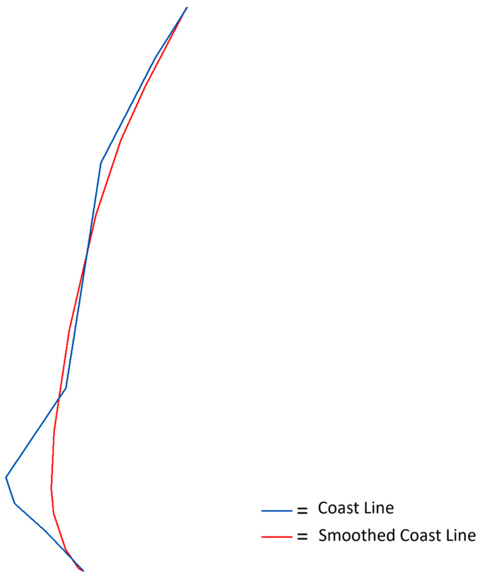
The flowchart in Figure 3 follows the flow as indicated by the arrows. The function in each submodule can be inferred from Figure 3 (as stated before, more details can be found elsewhere [42]), but some highlights of these submodules are given. In brief, the submodule “Coast lines” uses cartographic information to create shorelines for each beach and smooths them [43] by means of a polynomic approximation with an exponential core; this is illustrated in Figure 4. A smoothing parameter, PTS, is determined by GCIFS, which is empirically defined [42] as other empirical factors and considerations [42].

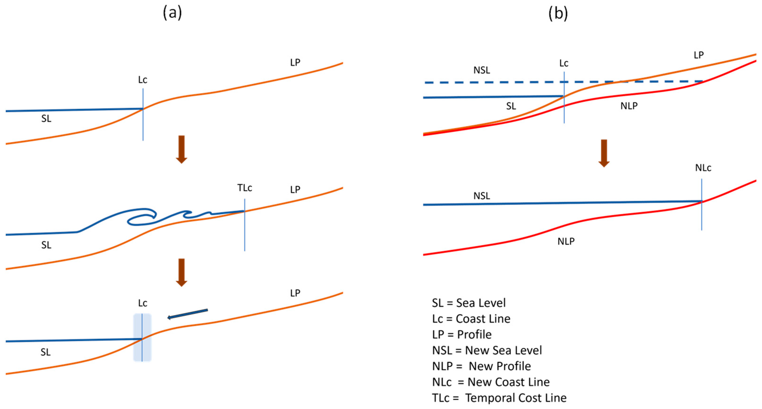
The submodule “Directions” in Figure 3 determines the directions for each individual shoreline. The term ‘Run-up’ [44], used for a flooding that occurs and ends in a very limited time period without modifying the geomorphology of the beach [44,45] (Figure 5a), was avoided. In this study, another erosion approach was pursued, since a modified long-term profile was required; such an approach implies a direction that will tend to create a new beach but preserve the original shape [46], as shown in Figure 5b. The profile shown in Figure 5 refers to the boundary between the longitudinal section between the beach and the ocean.

To apply the submodule “Directions”, several common parameters are required, as the beach secant, S, is given by

$$S=\frac{Y_1-Y_0}{X_1-X_0}$$

(1)

where X₀ and Y₀ and X₁ and Y₁ are the coordinates of the first and second points, respectively; its corresponding angle, SA, is computed as

SA = arctan(S)

(2)

The beach transversal (Equation (3)) is given below

$$Tr=arctan\left(\frac{-1}{S}\right)$$

(3)

and other parameters like the ocean location, beach orientation, and lateral extension; a direction correction was also carried out [42].

The submodule “LiDAR” in Figure 3 generates multivectors (multiple direction and altitude vectors) along each considered beach. A georeferenced shoreline is determined with unique vectors denoted as U-vectors, which have a common direction but with a unique varying elevation or depression; this was inspired by Cliord exterior algebra [14]. To do so, the Light detection and Ranging (LiDAR) technique is used [47]. Another important concept is the digital elevation model (DEM), which is created through direct field measurements using, for instance, topographic surveys with GPS and altimeters as well as several techniques to store them as raster images [48]. Since the advent of LiDAR radar, all DEMs with a resolution less than 5 × 5 m can be determined with this radar. It can be described as a high-resolution sensor, fixed or movable, that is provided with a pulse laser transmitter and a receptor [47]. For large land lengths, the georeferenced data are normally obtained in an air transported way (Figure 6a) or by scanning (Figure 6b).

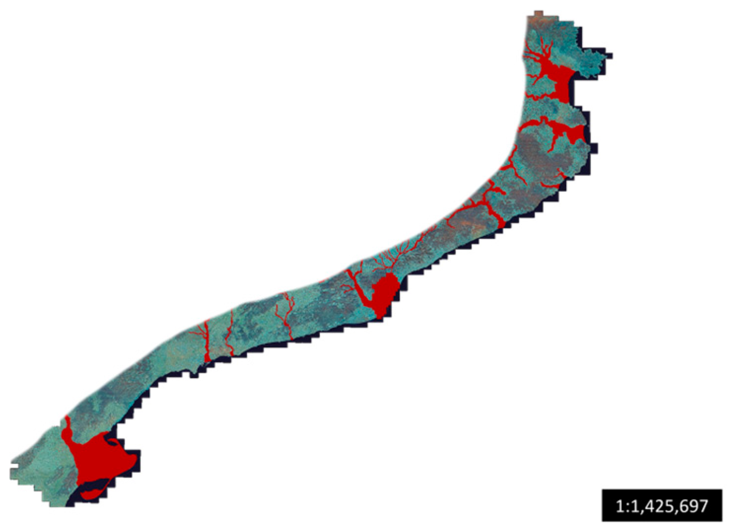
As previously mentioned, in the Catalonian cartographic system (CCS), all DEMs with a resolution less than 5 × 5 m are based on LiDAR radar, providing a resolution as high as 1 × 1 m in certain areas, as shown in Figure 7.

High-resolution data play a key role in the accurate estimation of erosion (or other climate change related phenomena), future shorelines, and associated costs, as stated above. In Catalonia, a database in a cloud with a minimum density of 0.5 points/m² is available for altimetry precision with an average 6 cm of quadratic error [49]. The original LiDAR files (raw data) are stored as the file type LAS (extension ‘.las’, the three first letters of laser; see also

Table 1. Erosion models.

Model	Description
Brunn5	Brunn’s law with an increase in the annual average sea level IPCC-RCP8.5
Brunn3	Brunn’s law with an increase in the annual average sea level IPCC-RCP4.5
Alde	Without an increase in the annual average sea level IPCC-RCP8.5
Erlv	Local erosion
Gcifsln	Maximum erosion for each multivector using the local erosion data

), the same as those generated by the American Society for Photogrammetry and Remote Sensing [50]. These LAS files are available as a compressed version in the file type LAZ (extension ‘.laz’), as created by the open project ‘LASzip’. [51]. The ‘Las_dataset’ (Table 1) is an independent file that creates references to every ‘.las’ file. 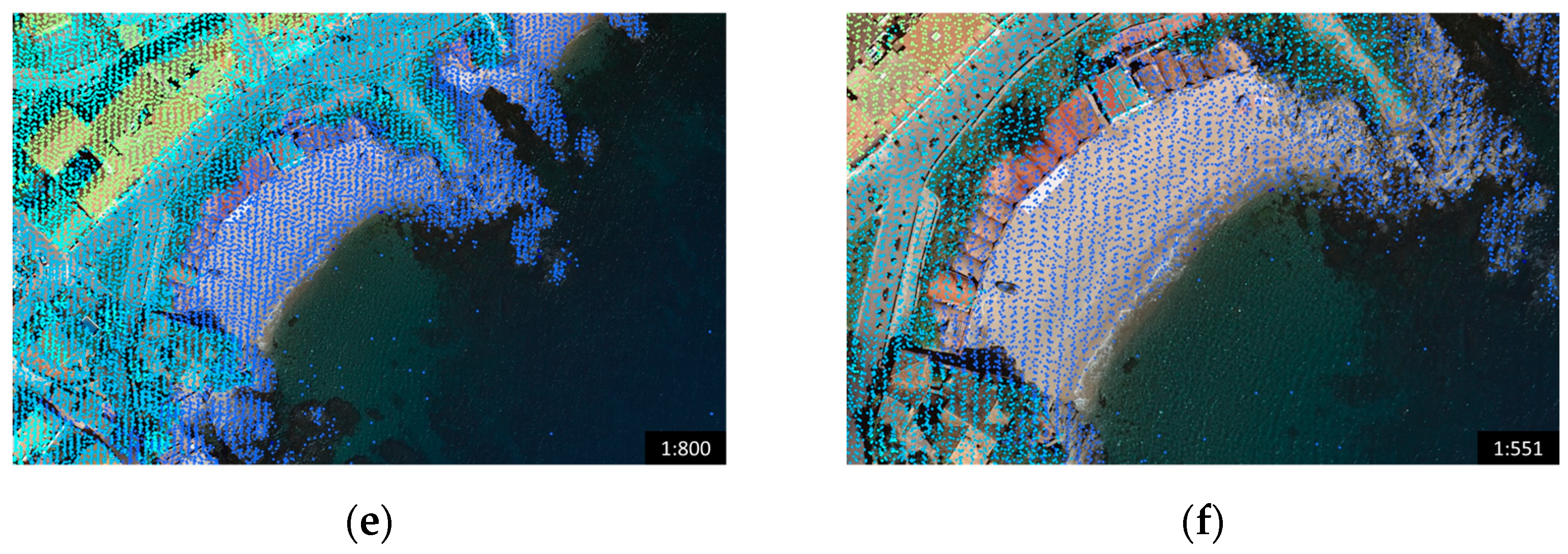A thorough description of the ‘Las_dataset’ is available in [42]; although this reference is in Spanish, the most relevant information is contained here as well as in the employed references (see the References section, together with an English translation of the title of [42]). An example of the processed images using these files is shown in Figure 8.

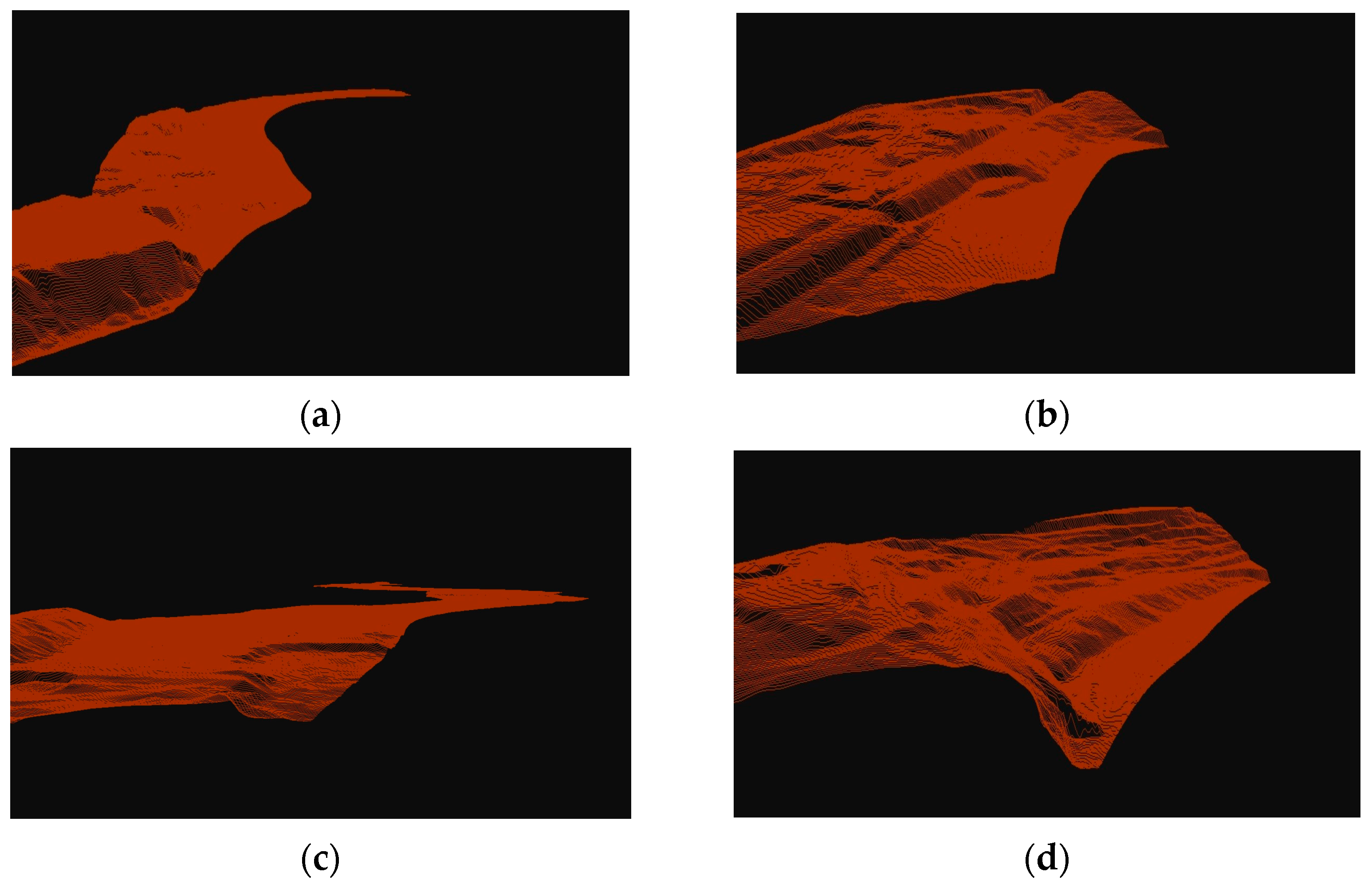
The LiDAR information is also used to create the multivectors, as schematically shown in Figure 9. The use of multivectors leads to real models like the one shown in Figure 10. More details can be found in [42].

The multivectors in turn allow for the use of the submodules “Polygons” and “Area under the curve” to generate base polygons such as those shown in Figure 11 as well as compute their corresponding areas by well-known numerical integration methods (e.g., Ref. [52]) and to delimit the beach regions.

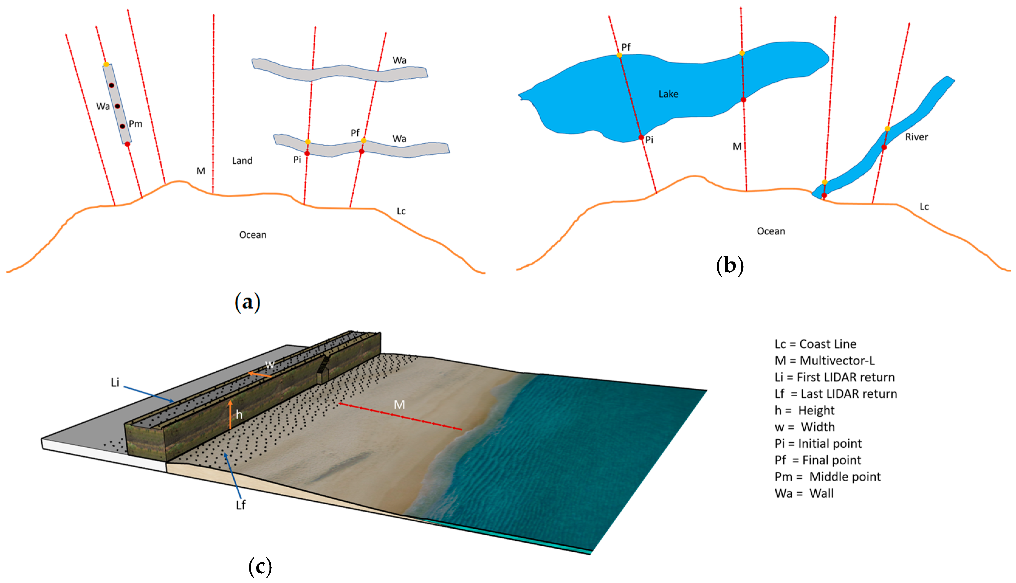
Finally, the submodules of GCIFS lab termed as “Walls” and “Water bodies” are used to identify, filter, and measure the existing walls (e.g., protection structures) and the water bodies in the area under study, respectively. This is schematically illustrated in Figure 12a–c.

This includes all submodules of GCIFS lab. The next module in Figure 2, termed as “GCIFS Analysis”, is described in the following.

“GCIFS Analysis” is the second module shown in Figure 2. It is in this module that the beaches are analyzed and the erosion computed. It uses the previous module information as input, which is also subdivided into submodules, as shown in Figure 13.

Rather than describing each submodule in Figure 13 (the names of the submodules are indicative of their purposes), a brief description of the salient points of the “GCIFS Analysis” is given below. The contact points can be determined using different erosion models, as listed in Table 1 [53].

The erosion is computed over the created scenarios based on the limiting distance of each multivector, from the current shoreline up to the predicted shoreline for a given year. This is determined for every beach for the Brunn5, Brunn3, and Alde models, for each beach for Erlv, and for each multivector in GCIFSln [53]. The Brunn5 and Brunn3 models are based on a limiting distance as per the maximum predictions of IPCC-RCP8.5 of an average sea level rise of 1 m and IPCC-RCP4.5 of 0.76 m, respectively; these correspond to the coast erosion estimated with Brunn’s law by Mimura and Nobuoka [53]. For the Alde model, the new shoreline is derived only for the average sea level rise IPCC-RCP8.5 without erosion. The Gcifsln model proposed in GCIFS determines a vectorial erosion capacity (VEC) factor for each multivector using the local annual erosion data. The factor is defined by the area under the curve of the multivector in the local erosion length. Subsequently, each contact line (second submodule in Figure 13) of each multivector is computed by means of the VEC factor for the desired year (Figure 14).

Two itinerancy systems for each multivector can be included or excluded without impacting the general procedure (Figure 15). One is Acba, a system that identifies possible geographical alterations of slow erosion like cliffs or large terrain volumes in short distances [54].

The other one is termed Walltsy, and it detects incomplete walls. If an incomplete wall is detected, Acba checks whether a difficult-to-erode geography is located behind the wall, and a factor to limit the water advance will be considered. In contrast, if the location is free, the erosion model applied at the time will be kept. This is illustrated in Figure 16a and Figure 16b, respectively.

If several beaches are analyzed simultaneously, the software is able to identify impact polygons that can be superposed and correct the neighbor polygons with this problem (Figure 17).

The model is originally designed to work with all of the required systems. So far, only two have been presented: (1) Acba, which allows for the identification of zones as cliffs with minimum erosion for the time period of interest, and (2) Walltsy, which allows for the identification and measurement of infrastructures (as provided by local cartography) as protection walls that limit the erosion of the zone. Both systems were used in this study as indicated, except for Brunn5_no and Brunn3_no, so that differences could be identified. If these (identification) systems are employed (i.e., Acba and Walltsy), more precise results can be obtained because these difficult-to-erode zones are identified. As shown later, this will have an impact on the costs (i.e., the total costs when these systems are employed are much lower because much more refined information is employed, and less infrastructure and regions are impacted). Not using these systems (i.e., using less precise information) will lead to an overestimation of the total costs, as expected.

All of the previous information can be used to compute the impact volumes for each segment, as shown in Figure 18, which in turn allows one to obtain the total impact volume by addition. GCIFS Analysis can also quantify segment areas, the impacted beach area in m², the intersection with the ocean, intersection with other water bodies, and the total erosion of the beach for a year.

The next module in Figure 2 is termed as “GCIFS Infra” and is described below.

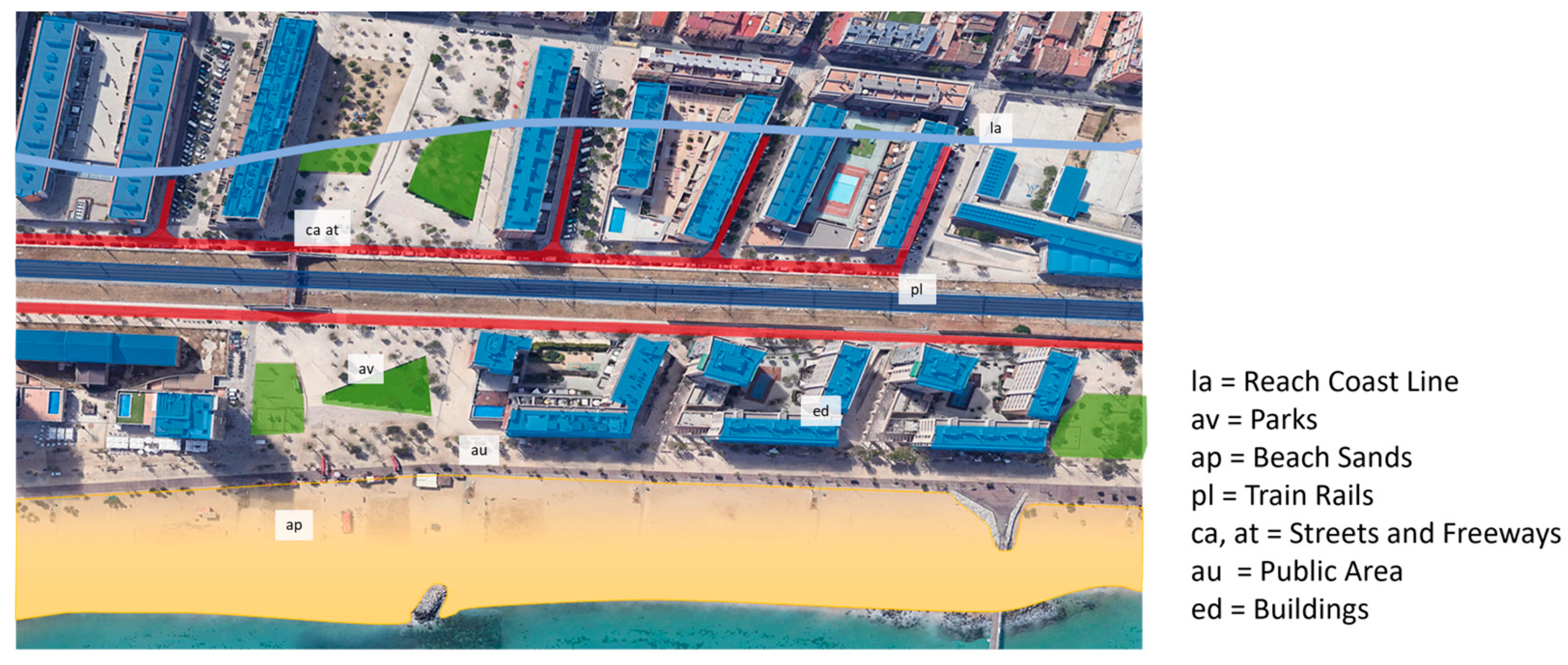
“GCIFS Infra” (the third module showed in Figure 2) is used to identify, classify, and measure the infrastructure in the impact zone for each analysis. This module uses the impact polygons defined earlier to first identify detailed impacts to the infrastructure of different types, namely gardens, sand beach, country, train, highways, streets, public areas, and buildings. Then, the area for all kinds and lengths of trains, highways, and streets is determined. Finally, for the specific case of buildings, these structures are delimited as complete units for a more detailed analysis to be explained right after the next GCIFS module (the fourth one in Figure 2). An example of the analysis of the impacted infrastructure is shown in Figure 19.

The “GCIFS buil” is represented in the fourth module shown in Figure 2. It is used to classify and determine the type, number of stories, and commercial areas of the buildings in a given impact polygon. The more detailed analysis of the buildings in this module is aimed at more accurately defining their importance and computing their costs. The module identifies the building as dwellings, hotels, commercial, schools, hospitals, historic, government, sport, factory, gas stations, and transportation stations. An example is illustrated in Figure 20. The Tax Agency of Catalonia [55] is used as the source to establish the average story height, percentage of each type of building considered as the commercial area, and other relevant parameters (see details in [42]). The last two modules of GCIFS are described in the following.

The “GCIFS protect” module is the fifth module shown in Figure 2. Its function is to determine the required protection length to avoid erosion after each sand beach. To do so, the existent functional walls are considered as well as the cliffs or upper lands. With this information, the protections are classified as without protection, incomplete protection, or complete protection. As with the other modules, extensive details, input and output file names, etc., were omitted for space reasons, but can be found in [42]. Instead, the procedure can be readily inspected in Figure 21 in a schematic manner. It should be noted that processes such as wave run-up on the beach and structures, overtopping, and structural condition assessment were omitted from this analysis.

The sixth and last module of the software is “GCIFS cost”, as shown in Figure 2. This module assesses the impact costs on the Catalonian coast based on the impacts and protections. It employs the previously generated information on the infrastructure, buildings, and protections for each zone. For a realistic cost evaluation, the time and inflation rates are considered. The main assumption is that when a zone in the neighborhood of the shoreline is lost, it will be necessary to relocate it; therefore, the current commercial cost is not considered, but the total reconstruction cost.

The GCIFS program (implicitly the described implemented methodology) was applied to a practical case in the next section. The selected region was the shoreline of Catalonia, and the results are given below.

3. Case-Study Data, Scenarios and Results for the Coast of Catalonia

3.1. Study Area

The coast of Catalonia is in the northwest Mediterranean region. Depending on the considered resolution, it can extend along approximately 580 km [56] to 780 km [57]. With almost eight million inhabitants, Catalonia is the second most populated autonomous region in Spain, with very high population density (around 240 inhabitants/km²; [58]). Catalonia is the second largest economy in Spain with a gross domestic product (GDP) of around EUR 230 million per year [59]. Figure 22 shows the Catalonian coast under study.

Approximately 70% of the population lives along a 20 km coast strip, and infrastructure and artificial beaches are located over approximately 152 km of coast [60]. Broadly speaking, the Catalonian coast can be divided in cliffs, rock beaches, and sand beaches; more details can be found elsewhere [57,61]. There is 172 km of coast being eroded [62] at different degrees of erosion [56].

3.2. Scenarios and Results

The GCIFS model was applied to the coast of Catalonia, as described above. More details and the results are presented in the following.

A total of 262 beaches, with at least one building behind the shoreline, was selected. A complete list can be found in [42], together with the extensive costs from different elements for different years as well as an appendix containing the resulting high-resolution and high-quality data and maps. In this study, we succinctly present the relevant information to show the adequacy of GCIFS and support our conclusions. Records were computed by decade from 2030 to 2100 in order to be consistent with those for the predictions of the IPCC for the increase in the average sea level with a maximum distance of 200 m per multivector. The topographic base used was 1:5000 (Cartographic and Geological System of Catalonia; CGSC). Orthophotos were from the raster server of CGSC “Catalunya 1:1000 vigent”. LiDAR was based on the CGSC: cloud with a minimum density of 0.5 points/m² and average quadratic error of 6 cm. The coordinate and vertical coordinate systems were ETRS_1989_UTM_Zone_31N and EPSG:5782 Alicante, respectively. The local erosion was based on the Catalonian “green book” on the state of coastal zones (CGSC, 2010).

The reference costs were based on different official sources. The infrastructure costs were based on the 2023 database of the Valencia Institute of Building ([63]; Catalonian section). These are listed in

Table 2. Reference cost of infrastructure in Catalonia.

Infrastructure	Cost
Parks	52.00 €/m2
Beach sands	16.89 €/m2
Train rails	1075.08 €/m
Streets	1038.70 €/m
Freeways	1465.44 €/m
Public area	66.00 €/m2

.

Costs for different types of buildings were based on [64] and are listed in

Table 3. Reference cost of buildings in Catalonia.

Buildings	Factor	Cost (€/m2)
Apartments	1.2	1224.95
Hotels	1.4	1429.15
Commercials	1.3	1327.06
Schools	1.0	1020.82
Hospitals	1.5	1531.23
Historical Buildings	1.0	1020.82
Factories	1.2	1224.95
Governments	0.6	612.45
Gas Stations	1.2	1224.95
Transport Stations	1.2	1224.95
Sport facilities	0.45	459.35

. A base cost of 1020.82 €/m² was considered and scaled according to the factor reported in Table 3. When applicable, this cost was in turn multiplied by the number of stories.

The costs of protections (simple walls and concrete walls with wave return were considered) were based on the Environment Agency UK Gov [65], as shown in

Table 4. Reference cost of coast protection.

Protection	Cost (€/m)
(I) Simple seawall	2176.00
(II) Concrete seawall with waves reflection	7166.08

.

It should be noted that all of the computed costs were approximated for the considered year by adding a 0.03% annual increment as per the average inflation, after the Organization for Economic Cooperation and Development [66].

Seven different scenarios, essentially analysis types, were performed with a complete GCIFS for each scenario on one or more beaches, depending on whether submodels and systems were applied or not. This is described in

Table 5. Analysis carried out in the study area.

Analysis	Description
Brunn5_no	Submodel Brunn 5 without systems
Brunn5_aw	Submodel Brunn 5 with the Acba and Walltsy systems
Brunn3_no	Submodel Brunn 3 without systems
Brunn3_aw	Submodel Brunn 3 with the Acba and Walltsy systems
Alde_aw	Submodel Alde with the Acba and Walltsy systems
Erlv_aw	Submodel Erlv with the Acba and Walltsy systems
Gcifsln_aw	Submodel Gcifsln with the Acba and Walltsy systems

, and a discussion and our conclusions in more general terms are provided later. Nevertheless, differences among all the models in Table 5 can be readily inspected in Figure 23, where it can be observed that deactivation of the Acba (to identify difficult-to-erode zones as cliffs) and Walltsy (to identify infrastructure and protection walls) systems led to an overlap of the projections for given decades (i.e., the predicted shoreline expected in that decade) over buildings and therefore higher impact costs, which did not occur when the Acba and Walltsy systems were considered. More details on each erosion model in Table 5 are also given (under Figure 17).

The results of the seven scenarios in Table 5 include the costs (or other parameters as length units as applicable) as a function of time (i.e., different projection decades) and they are depicted in figures and listed in tables [42] for four groups: (1) impacted areas, (2) impact costs, (3) total impact costs, and (4) protection costs. The impacted areas were subdivided into impacted zones, impacted infrastructure, and impacted buildings. The impact costs were subdivided into impacted infrastructure costs and impacted building costs. The total costs included the total costs of all infrastructure and the total costs of all buildings and the sum of both.

The previous subgroups were further divided into the other detailed information described previously. For instance, for the group of impacted areas and the subgroup impacted zones, there were results for the total area, water bodies, total volume, and sand volume. For the group of impacted areas and the subgroup of impacted infrastructure, there were results for parks, beaches, country, public areas, railway, streets, and so on. This has been extensively depicted and tabulated in [42]. In this study, for the sake of brevity, we only presented the results for the total costs and protection costs, since this is the information linked to the relevant conclusions stated later.

Figure 24 shows the total costs in million EUR of the impacted infrastructure as a function of projected time (from the year 2020 to year 2100); it can be observed that the case of Brunn5_no (Table 5) led to the largest costs; in contrast, the Alde_aw case (Table 5) generated the smallest costs. The amounts in EUR for each case are listed in

Table 6. Costs of the impacted infrastructure (millions of EUR).

Year	Brunn5_no	Brunn5_aw	Brunn3_no	Brunn3_aw	Erlv_aw	Alde_aw	Gcifsln_aw
2030	68.80	68.83	45.81	45.56	90.92	2.73	35.00
2040	172.81	167.83	112.32	110.98	185.76	4.07	69.73
2050	317.98	299.33	207.09	203.10	315.80	6.09	118.21
2060	525.43	466.76	346.06	327.93	461.88	9.34	180.82
2070	788.43	657.12	517.06	472.55	610.67	14.97	257.87
2080	1129.42	874.65	750.32	655.85	755.76	24.32	347.97
2090	1517.24	1095.63	100.07	840.43	900.31	40.31	450.28
2100	1971.35	1316.19	1328.20	1051.51	1046.28	63.48	564.12

. The other scenarios were between these bounds. It is expected that any analysis that did not include the systems (no; Table 5) yielded larger impact costs in comparison to those that did consider them (aw; Table 5). Figure 25 and Figure 26 and

Table 7. Costs of the impacted buildings (millions of EUR).

Year	Brunn5_no	Brunn5_aw	Brunn3_no	Brunn3_aw	Alde_aw	Erlv_aw	Gcifsln_aw
2030	198.06	112.12	70.62	63.91	63.45	0.00	1.01
2040	502.74	366.29	337.37	296.78	283.87	0.00	22.41
2050	1082.60	809.68	602.62	515.71	489.75	0.00	33.62
2060	1896.11	1336.97	1089.01	857.29	645.71	0.00	48.50
2070	2735.34	1687.93	1800.69	1330.79	1032.17	0.00	63.95
2080	3909.42	2111.35	2532.38	1797.58	1199.78	0.00	90.14
2090	5238.95	2526.87	3353.33	2129.80	1360.48	0.00	225.13
2100	6874.65	2894.83	4492.72	2535.85	1636.86	0.00	258.55

and

Table 8. Total costs of the impacted infrastructure and buildings (millions of EUR).

Year	Brunn5_no	Brunn5_aw	Brunn3_no	Brunn3_aw	Alde_aw	Erlv_aw	Gcifsln_aw
2030	266.86	180.86	116.43	109.47	154.37	2.73	36.01
2040	675.55	534.12	449.68	407.76	469.64	4.07	92.15
2050	1400.58	1109.01	809.71	718.81	805.55	6.09	151.84
2060	2421.54	1803.73	1435.07	1185.22	1107.59	9.34	229.32
2070	3523.78	2345.05	2317.75	1803.34	1642.83	14.97	321.81
2080	5038.84	2986.01	3282.70	2453.43	1955.53	24.32	438.11
2090	6756.19	3622.50	4359.40	2970.24	2260.78	40.31	675.41
2100	8846.00	4211.02	5820.92	3587.36	2683.14	63.48	822.67

are analogous to Figure 24 and Table 6, except that the former refer to impacted buildings and the latter to the total cost by adding the impacted infrastructure and impacted buildings. As can be seen, the trends were similar, but with the differences shown in the corresponding figures and tables. A discussion is given in the following section.

Finally, the protection costs for the selected decades are presented in

Table 9. Protection costs (millions of EUR).

Year	Protection I	Protection II
2030	449.39	1479.93
2040	560.80	1846.86
2050	672.22	2213.78
2060	783.64	2580.71
2070	895.06	2947.63
2080	1006.47	3314.56
2090	1117.89	3681.48
2100	1229.31	4048.41

. Protections I and II are as previously described.

CGIFS predicts that to protect all the infrastructure and facilities along the coast of Catalonia, a total of 407 seawalls are required, encompassing a length of 170,676 m.

The results of this study are discussed in the following.

4. Discussion

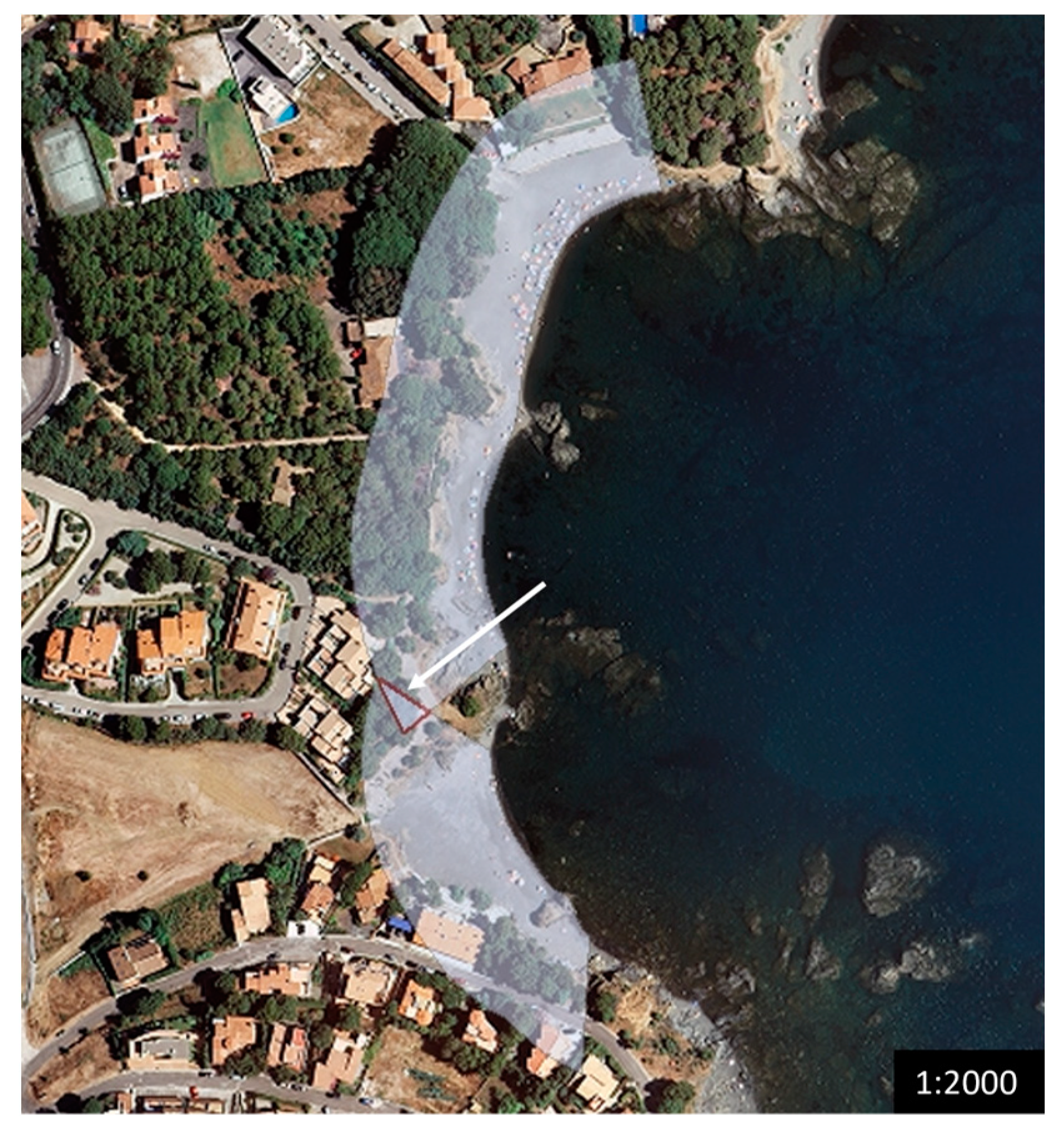
Noticeable differences were seen in the results of the study among the considered scenarios. As expected, methodologies that omitted the land characteristics and existent infrastructure led to results with a uniform trend, which significantly increased the loss of land and the costs. Consider, for example, the cases of Bruun5_no and the Brunn3_no (shown in Figure 27), where these differences were shown for beach p10 (Platja La Farella).

The general results of the study showed a wide variety in the impact costs for the year 2100, from EUR 63.84 to EUR 8846 million. However, apart from the Alde_aw case (determined through the increase in the average sea level), the Gcifsln_aw case showed the smallest impact, with a cost of EUR 822.67 million. It is noteworthy that this analysis case considered the local erosion and terrain by means of erosion factors; therefore, it is a feasible option for local studies in extensive areas, which is consistent with the main objective of this study.

Although cases Erlv_aw and Gcifsln_aw were based on local erosion as a reference, it can be observed that the latter generated less impact due to the variation in morphology for a given beach, where the erosion did not impact all points in a uniform way.

It was found that the inland water bodies (Figure 28) were not significantly impacted. This is understandable because there is a lack of them in the zone under study.

It was also noted that the Acba system led to a significant reduction in the loss of land where the soil is not erosion prone. Whether Acba is used or not, differences of approximately 50% were assessed. This suggests that if Acba is not employed, a significant overestimation in the results will be obtained.

The Walltsy system did not modify the results to a great extent, since no beach where the analysis was performed has a complete seawall to be effective as coastal protection. The existent seawalls only partially cover the zone, with no difficult-to-erode land behind them. None of the analyzed beaches has been provided with really efficient protection to avoid damage to the infrastructure and buildings near it.

In this study, infrastructures without any kind of impact in any analysis were excluded such as highways, schools, hospitals, factories, and gas stations. These results were visually verified using topographic maps; it was observed that along the coast of Catalonia, there are no highways closer than 200 m away from any beach. It was observed that some characteristics such as the type of building led to no impact at all. This is due to the fact that the study focused on the total functionality of the building. For instance, in the cases where a hospital or school was located on the ground floor of the building and the rest were dwellings, it was considered as a dwelling building with respect to the cost and functionality.

It was observed that the required number of contention seawalls (407) exceeded the number of studied beaches (262) because, as detailed in the GCIFS protect methodology, determining the required protection lengths for each beach was carried out considering the existing protective walls and/or cliffs or places with large cumulated land. Thus, the terrain was not considered and the required protection for a beach can result in one or several of shorter lengths, as illustrated in Figure 29.

Using the total cost of analysis as a reference for Brunn5_aw and Brunn3_aw, and comparing it with the Protection II type, it can be observed that they are similar and that the protect costs did not differ significantly. However, Erlv_aw and Gcifs_aw led to a difference of 50% and 25%, respectively.

Broadly speaking, the results show that when erosion predictions are considered in any analysis case, the infrastructure is invariably impacted, and the costs significantly increase.

Although the main features of GCIFS were not described in the previous section in this manuscript, we mention here that the software includes completely automatized procedures, avoiding the manual usage of a georeferenced system such as ArcMap^® or Qgis^®; the results are also reported automatically. The only required inputs are the data, and output databases, shapefiles, tables, figures, and spreadsheets will be generated. The program is very versatile and can easily be adapted to any available information and any beach around the world, from 1 m to a whole shoreline for the desired characteristics such as geographic location, morphology, infrastructure, orientation, etc. All shapefiles can be easily retrieved through a unique code. The process can be sped-up if information on the desired place is already loaded. GCIFS can be used on any ordinary computer with regular computing power; all procedures are performed in chain without overloading the RAM memory or at high speed, where procedures are performed in blocks. GCIFS can be modified for any specific purpose. The model employs the files and denotations listed in

Table 10. Files and denotations employed in GCIFS.

Abbreviation	Description
SH	Shapefile
AT	Arcpy tool
DB	Data base
IDB	Incidence data base
LD	Las_dataset
aw	Acba_walltsy

.

Note the fact that more accurate local information avoids an inadequate cost evaluation that can be investigated by comparing the use of DEM versus LiDAR data; the interested reader is referred to references provided in the Introduction. Nevertheless, future research is recommended to further investigate this aspect.

5. Conclusions

A tool in Python named GCIFS (Georeferenced Impact Forecast System) was developed to evaluate the impact cost on coasts due to climate change, which was based on LiDAR technology as well as cartography, online databases, and other sources of information. It was used to predict future shorelines and economic impacts on the coast of Catalonia and its infrastructure. The innovative methodology includes unique beach-specific cases and analysis scenarios and multivectors (multiple direction and altitude vectors) to identify regions that are difficult to erode as well as the existing protective seawalls. Seven analysis cases based on sea-level rise information by including/excluding coastal geomorphology were applied to the beaches along the coast of Catalonia.

Climate change is a reality and its impacts on coasts from a physics standpoint (receding shoreline, loss of sediments, increased flood risk, more vulnerability, loss of land, economic and functionality losses) will be very significant as well as the impact and/or protective measures costs. In this study, it was found that 100% of the analyzed beaches will be partially or totally impacted by the average sea level increase. The most significant impact costs for infrastructure corresponded to sand beaches, public areas, and streets, while the costs associated with parks and railways were much lower. For instance, in the worst-case scenario (Brunn5_no), the impact cost on sand beaches will increase from EUR 48.48 million in 2030 to EUR 611.40 million in 2100. The largest increases will be in 2050 for sand beaches, in 2070 for parks and railways, and in 2090 for streets. This order in the impact is expected because of the geographic location with respect to the shoreline. Also, it should be considered that some types of infrastructure such as parks and railways may not exist at all beaches.

If the buildings are taken into account, all scenarios show that dwellings, hotels, and commercial buildings will be the most impacted by the loss of coast, thus leading to the highest impact costs. It can be concluded that the impact costs will be relatively small in the decade starting from 2030, but will significantly increase in the subsequent decades, especially in the worst-case scenario where the impact cost to dwellings will experience the highest cost increase from EUR 178.14 million in 2030 to EUR 5818.49 million in 2100.

A less conservative analysis by considering the coast morphology (Brunn3_aw) led to a similar behavior with respect to the worst-case scenario, but with much smaller impact costs. For example, the impact cost to dwelling buildings will increase from EUR 46.96 million in 2030 to EUR 2094.27 million in 2100. Also, the hotels and commercial buildings will exhibit a gradual increase, with commercial buildings being the most impacted. A noteworthy difference in both analyses is that only the former indicated the impact costs to historic, government, sport buildings, and stations, which suggests that these structures are not near the coast zone under study.

In all of the analyzed cases, a continuous increase over time in the impact costs for buildings was found. This is because the region under study is large and densely populated, with several buildings near the coast of Catalonia. As the shoreline recedes, it is expected that more buildings will be impacted over time. In contrast to densely populated beaches with many buildings in a coast strip about the shoreline such as in tourism zones, as the density diminishes and the infrastructure is further away from the coast, the impact costs for buildings are expected to be less significant.

Based on the results of the study along the coast of Catalonia, it can be concluded that there is a large variability in impact cost, depending on the considered analysis and the available information; detailed information with high quality and resolution as well as advanced technology play a key role in obtaining adequate predictions. If only the average sea level increase is considered, the study shows that in 2100, the total impact cost will be EUR 63.48 million, which differs significantly from the EUR 8846.00 million total impact cost for the same year, if the worst-case scenario, without taking into account the geomorphology, is to be considered. If the geomorphology is included in the worst-case scenario as well as the existent protective seawalls, the impact cost is reduced by 50%; the main reason for this difference is that difficult-to-erode zones are excluded in a very conservative analysis.

It was also concluded that by including the local erosion measures, the costs decrease. Once more, this shows the importance of using precise information with the highest possible resolution to assess the impact cost due to climate change on beaches, together with their infrastructure, buildings, and protection walls, which was the case for the average sea level rise and erosion, but it could also be the case for other parameters. This is a very important conclusion because the better the input information provided to the innovative GCIFS (Georeferenced Impact Forecast System) software developed in this study, the more adequate the predictions will be, which will have significant implications in coastal management and protection.

This study also found that a large investment is required to protect the infrastructure behind Catalonian beaches. If the most conservative models are considered such as those developed in the submodels Erlv and Gcifsln in GCIFS, such an investment would be unfeasible. The developed program showed its efficiency in creating individual scenarios for each beach, providing a large amount of data while maintaining computing efficiency (using common computers) and the ability to perform analysis for different erosion theories and receding of the shoreline. It was observed that the differences when considering the geomorphology or not were very large for assessing the loss of land due to the average sea level increase for the following years. Therefore, inclusion of the geomorphology was found to be critical for adequate evaluations of the impact costs on coasts. The methodology to assess the shoreline receding by means of a direction from the shoreline itself, as carried out in GCIFS, proved to be optimal to avoid wrong flood predictions. This is relevant for assessing the impacted areas and impact costs as well as developing risk maps. The software also showed its ability to adapt to any type of morphology and obtain high-resolution data and maps by using online information and updating files, which is critical to keep the information updated. It is also able to adapt the available information of any source type.

It is evident that decision making in terms of providing resources to protect coasts includes a wide range of subjects, results, and experts with different backgrounds. However, the employment of new methodologies and technologies that are able to provide better information, in quantitative and qualitative terms, will lead to more resilient solutions. GCIFS could be used to face future challenges for any coast worldwide, and it is a very valuable tool for coastal engineers, researchers, and code developers as well as for government, insurance, and private sectors interested in the impact costs on coasts due to climate change.

As a final remark, it is noted that even though the advantages of the developed software have been highlighted together with the statement that any type of information can potentially be adapted to it, researchers and practicing engineers should always bear in mind that there is no software that can cover all possible issues arising from every considered coast around the world, and that the lack of information and its wide variety may limit the use of computer programs. Also, it is emphasized that tools cannot replace the ability of practicing coastal engineers and that care should be exercised when using any software tool. The experience of a coastal engineer is always a key aspect for adequate design, who should also recognize that our knowledge is always limited and that the epistemic uncertainties can be large.

References

1. IPCC. Climate Change_The Physical Science Basis; IPCC: Geneva, Switzerland, 2013; Volume 43. [Google Scholar]
2. Simas, T.; Nunes, J.P.; Ferreira, J.G. Effects of global climate change on coastal salt marshes. Ecol. Model. 2001, 139, 1–15. [Google Scholar] [CrossRef]
3. Hunt, A.; Watkiss, P. Climate change impacts and adaptation in cities: A review of the literature. Clim. Chang. 2011, 104, 13–49. [Google Scholar]
4. Maribus. World Ocean Review. 2017. Available online: https://worldoceanreview.com/en/wor-5/ (accessed on 1 October 2021).
5. Williams, S.J. Sea-level rise implications for coastal regions. J. Coast. Res. 2013, 63, 184–196. [Google Scholar] [CrossRef]
6. Reay, D.; Sabine, C.; Smith, P.; Hymus, G. Intergovernmental Panel on Climate Change. Fourth Assessment Report; Inter-Gov-Ernmental Panel on Climate Change: Geneva, Switzerland; Cambridge University Press: Cambridge, UK, 2007; Available online: www.ipcc.ch (accessed on 15 January 2022).
7. Steininger, K.W.; König, M.; Bednar-Friedl, B.; Kranzl, L.; Loibl, W.; Prettenthaler, F. Economic Evaluation of Climate Change Impacts; Springer: Berlin/Heidelberg, Germany, 2015. [Google Scholar]
8. Petrişor, A.-I.; Hamma, W.; Nguyen, H.D.; Randazzo, G.; Muzirafuti, A.; Stan, M.-I.; Tran, V.T.; Aştefănoaiei, R.; Bui, Q.-T.; Vintilă, D.-F.; et al. Degradation of Coastlines under the Pressure of Urbanization and Tourism: Evidence on the Change of Land Systems from Europe, Asia and Africa. Land 2020, 9, 275. [Google Scholar] [CrossRef]
9. Ciscar, J.-C.; Iglesias, A.; Feyen, L.; Szabó, L.; Van Regemorter, D.; Amelung, B.; Nicholls, R.; Watkiss, P.; Christensen, O.B.; Dankers, R.; et al. Physical and economic consequences of climate change in Europe. Proc. Natl. Acad. Sci. USA 2011, 108, 2678–2683. [Google Scholar] [CrossRef] [PubMed]
10. Hinkel, J.; Nicholls, R.J.; Vafeidis, A.T.; Tol, R.S.; Avagianou, T. Assessing risk of and adaptation to sea-level rise in the European Union: An application of DIVA. Mitig. Adapt. Strateg. Glob. Chang. 2010, 15, 703–719. [Google Scholar] [CrossRef]
11. Rizzi, J.; Torresan, S.; Zabeo, A.; Critto, A.; Tosoni, A.; Tomasin, A.; Marcomini, A. Assessing storm surge risk under future sea-level rise scenarios: A case study in the North Adriatic coast. J. Coast. Conserv. 2017, 21, 453–471. [Google Scholar]
12. Hereher, M.E. Vulnerability assessment of the Saudi Arabian Red Sea coast to climate change. Environ. Earth Sci. 2016, 75, 1–13. [Google Scholar]
13. Moftakhari, H.R.; AghaKouchak, A.; Sanders, B.F.; Feldman, D.L.; Sweet, W.; Matthew, R.A.; Luke, A. Increased nuisance flooding along the coasts of the United States due to sea level rise: Past and future. Geophys. Res. Lett. 2015, 42, 9846–9852. [Google Scholar] [CrossRef]
14. Vitousek, S.; Barnard, P.L.; Fletcher, C.H.; Frazer, N.; Erikson, L.; Storlazzi, C.D. Doubling of coastal flooding frequency within decades due to sealevel rise. Sci. Rep. 2017, 7, 1399. [Google Scholar] [CrossRef] [PubMed]
15. Hird, S.; Stokes, C.; Masselink, G. Emergent coastal behaviour results in extreme dune erosion decoupled from hydrodynamic forcing. Mar. Geol. 2021, 442, 106667. [Google Scholar] [CrossRef]
16. Luijendijk, A.; Hagenaars, G.; Ranasinghe, R.; Baart, F.; Donchyts, G.; Aarninkhof, S. The State of theWorld’s Beaches. Sci. Rep. 2018, 8, 6641. [Google Scholar] [CrossRef]
17. Vousdoukas, M.I.; Mentaschi, L.; Voukouvalas, E.; Verlaan, M.; Jevrejeva, S.; Jackson, L.P.; Feyen, L. Global probabilistic projections of extreme sea levels show intensication of coastal ood hazard. Nat. Commun. 2018, 9, 2360. [Google Scholar] [CrossRef]
18. Nerem, R.S.; Beckley, B.D.; Fasullo, J.T.; Hamlington, B.D.; Masters, D.; Mitchum, G.T. Climate-changedriven accelerated sea-level rise detected in the altimeter era. Proc. Natl. Acad. Sci. USA 2018, 115, 2022–2025. [Google Scholar] [CrossRef]
19. Mölter, T.; Schindler, D.; Albrecht, A.T.; Kohnle, U. Review on the Projections of Future Storminess over the North Atlantic European Region. Atmosphere 2016, 7, 60. [Google Scholar] [CrossRef]
20. Frieler, K.; Lange, S.; Piontek, F.; Reyer, C.P.O.; Schewe, J.; Warszawski, L.; Zhao, F.; Chini, L.; Denvil, S.; Emanuel, K.; et al. Assessing the impacts of global warming-simulation protocol of the Inter-Sectoral Impact Model Intercomparison Project (ISIMIP2b). Geosci. Model Dev. 2017, 10, 4321–4345. [Google Scholar]
21. Vousdoukas, M.I.; Ranasinghe, R.; Mentaschi, L.; Plomaritis, T.A.; Athanasiou, P.; Luijendijk, A.; Feyen, L. Sandy coastlines under threat of erosion. Nat. Clim. Chang. 2020, 10, 260–263. [Google Scholar]
22. Almeida, L.P.; Efraim de Oliveira, I.; Lyra, R.; Scaranto Dazzi, R.L.; Martins, V.G.; Henrique da Fontoura Klein, A. Coastal Analyst System from Space Imagery Engine (CASSIE): Shoreline management module. Environ. Model. Softw. 2021, 140, 105033. [Google Scholar] [CrossRef]
23. Fogarin, S.; Zanetti, M.; Dal Barco, M.K.; Zennaro, F.; Furlan, E.; Torresan, S.; Pham, H.V.; Critto, A. Combining remote sensing analysis with machine learning to evaluate short-term coastal evolution trend in the shoreline of Venice. Sci. Total Environ. 2023, 859, 160293. [Google Scholar] [CrossRef] [PubMed]
24. Martínez, M.L.; Intralawan, A.; Vázquez, G.; Pérez-Maqueo, O.; Sutton, P.; Landgrave, R. The coasts of our world: Ecological, economic and social importance. Ecol. Econ. 2007, 63, 254–272. [Google Scholar]
25. Doukakis, E. Coastal Vulnerability and Risk Parameters. Eur. Water 2005, 11, 3–7. [Google Scholar]
26. Mukhopadhyay, A.; Mukherjee, S.; Mukherjee, S.; Ghosh, S.; Hazra, S.; Mitra, D. Automatic shoreline detection and future prediction: A case study on Puri coast, Bay of Bengal, India. Eur. J. Remote Sens. 2012, 45, 201–213. [Google Scholar]
27. Hzami, A.; Heggy, E.; Amrouni, O.; Mahé, G.; Maanan, M.; Abdeljaouad, S. Alarming coastal vulnerability of the deltaic and sandy beaches of North Africa. Sci. Rep. 2021, 11, 2320. [Google Scholar]
28. Montaño, J.; Coco, G.; Antolínez, J.A.A.; Beuzen, T.; Bryan, K.R.; Cagigal, L.; Castelle, B.; Davidson, M.A.; Goldstein, E.B.; Ibaceta, R.; et al. Blind testing of shoreline evolution models. Sci. Rep. 2020, 10, 2137. [Google Scholar]
29. Vale, P.M. The changing climate of climate change economics. Ecol. Econ. 2016, 121, 12–19. [Google Scholar]
30. Brouwer, R.; Schaafsma, M. Modelling risk adaptation and mitigation behaviour under different climate change scenarios. Clim. Chang. 2013, 117, 11–29. [Google Scholar]
31. Frihy, O.E.; El-Sayed, M.K. Vulnerability risk assessment and adaptation to climate change induced sea level rise along the Mediterranean coast of Egypt. Mitig. Adapt. Strateg. Glob. Chang. 2013, 18, 1215–1237. [Google Scholar]
32. Thirumurthy, S.; Jayanthi, M.; Samynathan, M.; Duraisamy, M.; Kabiraj, S.; Anbazhahan, N. Multi-criteria coastal environmental vulnerability assessment using analytic hierarchy process based uncertainty analysis integrated into GIS. J. Environ. Manag. 2022, 313, 114941. [Google Scholar]
33. Brown, S.; Nicholls, R.J.; Lowe, J.A.; Hinkel, J. Spatial variations of sea-level rise and impacts: An application of DIVA. Clim. Chang. 2016, 134, 403–416. [Google Scholar]
34. Vafeidis, A.T.; Nicholls, R.J.; McFadden, L.; Tol, R.S.J.; Hinkel, J.; Spencer, T.; Grashoff, P.S.; Boot, G.; Klein, R.J.T. A New Global Coastal Database for Impact and Vulnerability Analysis to Sea-Level Rise. J. Coast. Res. 2008, 24, 917–924. [Google Scholar]
35. Diaz, D.B. Estimating global damages from sea level rise with the Coastal Impact and Adaptation Model (CIAM). Clim. Chang. 2016, 137, 143–156. [Google Scholar]
36. Santos, M.; Del Río, L.; Benavente, J. GIS-based approach to the assessment of coastal vulnerability to storms. Case study in the Bay of Cádiz (Andalusia, Spain). J. Coast. Res. 2013, 65, 826–831. [Google Scholar] [CrossRef]
37. Alves, F.L.; Coelho, C.; Coelho, C.D.; Pinto, P. Modelling coastal vulnerabilities-Tool for decision support system at inter-municipality level. J. Coast. Res. 2011, 64, 966–970. [Google Scholar]
38. Zhang, K. Analysis of non-linear inundation from sea-level rise using LIDAR data: A case study for South Florida. Clim. Chang. 2011, 106, 537–565. [Google Scholar]
39. Malik, A.; Abdalla, R. Geospatial modeling of the impact of sea level rise on coastal communities: Application of Richmond, British Columbia, Canada. Model. Earth Syst. Environ. 2016, 2, 146. [Google Scholar]
40. Seenath, A.; Wilson, M.; Miller, K. Hydrodynamic versus GIS modelling for coastal flood vulnerability assessment: Which is better for guiding coastal management? Ocean. Coast. Manag. 2016, 120, 99–109. [Google Scholar]
41. Palaseanu-Lovejoy, M.; Danielson, J.; Thatcher, C.; Foxgrover, A.; Barnard, P.; Brock, J.; Young, A. Automatic delineation of seacliff limits using lidar-derived high-resolution DEMs in southern California. J. Coast. Res. 2016, 76, 162–173. [Google Scholar]
42. Lomelí-Quintero. El costo del Impacto Sobre el Litoral Debido al Cambio Climático en Cataluña (The Cost of the Impact on the Shoreline Due to Climate Change in Catalonia). Ph.D. Thesis, Departamento de Ingeniería Civil y Ambiental, UPC, Barcelona, Spain, 2023. [Google Scholar]
43. Bodansky, E.; Gribov, A.; Pilouk, M. Smoothing and compression of lines obtained by raster-to-vector conversion. In Proceedings of the Graphics Recognition Algorithms and Applications: 4th International Workshop, GREC 2001, Kingston, ON, Canada, 7–8 September 2002; Lecture Notes in Computer Science. Volume 2390, pp. 256–265. [Google Scholar]
44. Hammeken Arana, A. Wave Run-Up on Beaches and Coastal Structures. Ph.D. Thesis, UCL (University College London), London, UK, 2017; p. 356. [Google Scholar]
45. Pakoksung, K.; Suppasri, A.; Imamura, F. Systematic Evaluation of Different Infrastructure Systems for Tsunami Defense in Sendai City. Geosciences 2018, 8, 173. [Google Scholar]
46. Bruun, P. Sea-Level Rise as a Cause of Shore Erosion. J. Waterw. Harb. Div. 1962, 88, 117–130. [Google Scholar]
47. Peralta Higuera, A.; Ramírez Beltrán, M.Á. Los Datos LIDAR: Nuevas Interacciones Entre la Geografía y las Tecnologías Avanzadas. In Geografía de México: Una Reflexión Espacial Contemporánea; UNAM: Ciudad de México, México, 2016; pp. 341–353. [Google Scholar]
48. Santaella, J. Modelos Digitales de Elevación (MDE); Instituto Nacional de Estadística y Geografía: Mexico City, Mexico, 2016; pp. 1–14. [Google Scholar]
49. ICGC. Dades LIDAR. 2023. Available online: https:www.icgc.cat/Administracio-iempresa/Descarregues/Elevacions/Dades-lidar (accessed on 20 August 2023).
50. ASPRS. Last Specification; Technical Report; American Society for Photogrammetry and Remote Sensing: Bethesda, MD, USA, 2013. [Google Scholar]
51. Isenburg, M. LASzip. 2019. Available online: https:laszip.org (accessed on 20 August 2023).
52. Quezada, R.; Domínguez, J. Un Estudio a la Integral de Riemann-Stieltjes. Ph.D. Thesis, Universidad del Bío-Bío, Concepción, Chile, 2020. [Google Scholar]
53. Mimura, N.; Nobuoka, H. Verification of the Bruun rule for the estimation of shoreline retreat caused by sea-level rise. In Proceedings of the Coastal Dynamics-Proceedings of the International Conference, Gdansk, Poland, 4–8 September 1995; pp. 607–616. [Google Scholar]
54. Pereira, C.; Coelho, C. Mapping erosion risk under different scenarios of climate change for Aveiro coast, Portugal. Nat. Hazards 2013, 69, 1033–1050. [Google Scholar]
55. Agencia Tributaria de Cataluña. Valors Bàsics dels Immobles Urbans. 2023. Available online: https://atc.gencat.cat/ca/normativa-i-criteris/valoracions-immobiliaries/valors-basics/ (accessed on 20 August 2023).
56. Roca, E.; Julià-Verdaguer, A.; Villares, M.; Rosas-Casals, M. Applying network analysis to assess coastal risk planning. Ocean. Coast. Manag. 2018, 162, 127–136. [Google Scholar]
57. Sánchez-arcilla, A.; Mösso, C.; Pau, J.; Casas, M. La Variabilitat Climàtica i la Costa Catalana. 2n Informe Sobre el Canvi Climàtic a Catalunya. Generalitat de Catalunya, Generalita. 2012, pp. 343–371. Available online: https://cads.gencat.cat/ca/publicacions/informes-sobre-el-canvi-climatic-a-catalunya/segon-informe-sobre-el-canvi-climatic-a-catalunya/ (accessed on 20 August 2023).
58. Núria, B.; Espasa, M. La Viabilidad Económica de una Cataluña Independiente. 2014. Available online: https://www.redalyc.org/pdf/969/96930463006.pdf (accessed on 20 August 2023).
59. Generalidad de Cataluña. Resumen del Informe Anual de la Economía Catalana 2020. Departamento de Economía y Hacienda. 2021, p. 17. Available online: https://economia.gencat.cat/web/.content/70_economia_catalana/arxius/informe-anual/informe-anual-2020/IA-2020-resum-es.pdf (accessed on 20 August 2023).
60. Guillén, J. Los Riesgos Litorales en Cataluña. Informe RISKAT. Los Riesgos Naturales en Cataluña; Generalidad de Cataluña; Consejo Asesor del Desarrollo Sostenible: Santander, Spain, 2008; pp. 1–26. [Google Scholar]
61. Casas-Prat, M.; Sierra, J.P. Trend analysis of wave direction and associated impacts on the Catalan coast. Clim. Chang. 2012, 115, 667–691. [Google Scholar]
62. Bosom, E.; Jiménez, J.A. Probabilistic coastal vulnerability assessment to storms at regional scale application to Catalan beaches (NW Mediterranean). Nat. Hazards Earth Syst. Sci. 2011, 11, 475–484. [Google Scholar] [CrossRef]
63. IVE. Base de Datos de Construccion. 2022. Available online: https://bdc.f-ive.es/BDC22/1 (accessed on 20 August 2023).
64. Royal Decree 1020/1993, a Boulletin (Boletín Económico de la Construcción, Construc, Eme Dos y Precios de Referencia de obra nueva de Edificación) from the Catalonian Technology Institute Available in “Basic Values of Urban Facilities” in the Taxes Agency of Catalonia (TAC, 2023). Available online: https://atc.gencat.cat/web/.content/documents/valoracions/vbasics/2023/valors_basics_urbana_catalunya_2023.pdf (accessed on 20 August 2023).
65. Hudson, T.; Keating, K.; Petit, A. Cost Estimation for Coastal Protection-Summary of Evidence; Environment Agency: Bristol, UK, 2015; p. 37. [Google Scholar]
66. OECD. Economics Inflation CPI. 2023. Available online: https://www.oecd-ilibrary.org (accessed on 20 August 2023).
Figure 1. The basic processes in GCIFS.
Jmse 11 01939 g001
Figure 2. Basic modules in GCIFS.
Jmse 11 01939 g002
Figure 3. Submodules of GCIFS lab.
Jmse 11 01939 g003
Figure 4. Zoom smoothed shoreline.
Jmse 11 01939 g004
Figure 5. (a) Run-up and (b) coast erosion.
Jmse 11 01939 g005
Figure 6. (a) Air transported LiDAR; (b) scanning LiDAR.
Jmse 11 01939 g006
Figure 7. Zones within a DEM at a 1 × 1 m resolution available in the Catalonian Cartographic System.
Jmse 11 01939 g007
Figure 8. LiDAR section. Beaches: (a) several, (b) several, (c) p44 (Platja Canadell), p45 (Calellade Palafrugell), p46 (Platja dels Burricaires), p203 (s/n), and p204 (Cala de Sant Roc), (d) p46, (e) p46, (f) p46.
Jmse 11 01939 g008aJmse 11 01939 g008b
Figure 9. Multivectors.
Jmse 11 01939 g009
Figure 10. Examples of real models: (a) Beach p91 (Platja de la Fragata), (b) beach p105 (Platya Savinosa), (c) beach p116 (Platya de I’Arenal) and (d) beach p243 (Platya Llarga).
Jmse 11 01939 g010
Figure 11. Examples of base polygons. Beaches (a) p25 (Cala Montjoi), (b) p28 (Platja dels Palangrers), (c) p29 (Platja Nov), and (d) p39 (Platja Fonda).
Jmse 11 01939 g011
Figure 12. (a) Wall identification, (b) Detection of water bodies and (c) Wall geometry.
Jmse 11 01939 g012
Figure 13. Processes for submodules in GCIFS analysis.
Jmse 11 01939 g013
Figure 14. Gcifsln methodology and VEC.
Jmse 11 01939 g014
Figure 15. Comparison of beach p0 (Platja de Portbou). Without Acba (a), with Acba (b).
Jmse 11 01939 g015
Figure 16. Walltsy, (a) High ground detection after the wall, (b) No high ground detection after the wall.
Jmse 11 01939 g016
Figure 17. Conflicting area in neighbor polygons.
Jmse 11 01939 g017
Figure 18. Impact volumes.
Jmse 11 01939 g018
Figure 19. Example of the impacted infrastructure analysis.
Jmse 11 01939 g019
Figure 20. (a) Number of stories (elevation) and (b) buildings Identification (plan view).
Jmse 11 01939 g020
Figure 21. (a) Required protections; (b) complete protection.
Jmse 11 01939 g021
Figure 22. Coast of Catalonia.
Jmse 11 01939 g022
Figure 23. Example of the models in Table 5 applied to p0 (Platya de Portbou): (a) Brunn5_no, (b) Brunn5_aw, (c) Brunn3_no, (d) Brunn3_aw, (e) Alde_aw, (f) Erlv_aw, (g) Gcifsln_aw.
Jmse 11 01939 g023
Figure 24. Costs of the impacted infrastructure.
Jmse 11 01939 g024
Figure 25. Costs of the impacted buildings.
Jmse 11 01939 g025
Figure 26. Total costs of the impacted infrastructure and buildings.
Jmse 11 01939 g026
Figure 27. Beach p10 (Platja La Farella) with and without systems: (a) Brunn5_no and (b) Brunn5_aw.
Jmse 11 01939 g027
Figure 28. (a) Distance to the inland body water closest to beach p104 (Platja Llarga) 7.5 km, (b) p149 (Cala Jovera) 7.8 km, and (c) inland body of water.
Jmse 11 01939 g028
Figure 29. Results of GCIFS protect for beaches (a) p0 (Platja de Portbou), (b) p23 (Platja sa Conca), (c) p28 (Platja dels Palangrers), and (d) p31 (La Platja de Les Barques).
Jmse 11 01939 g029