
Predictions of Wave Overtopping Using Deep Learning Neural Networks

Abstract
:1. Introduction
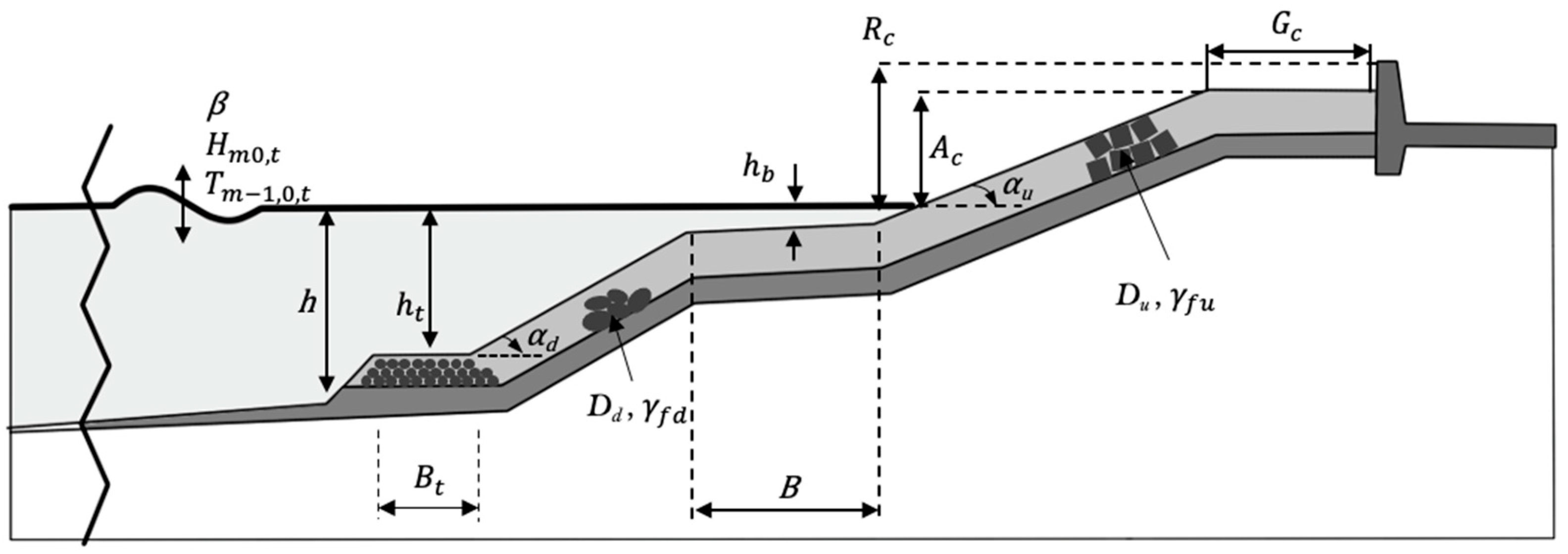
2. EurOtop Database
3. Method Description
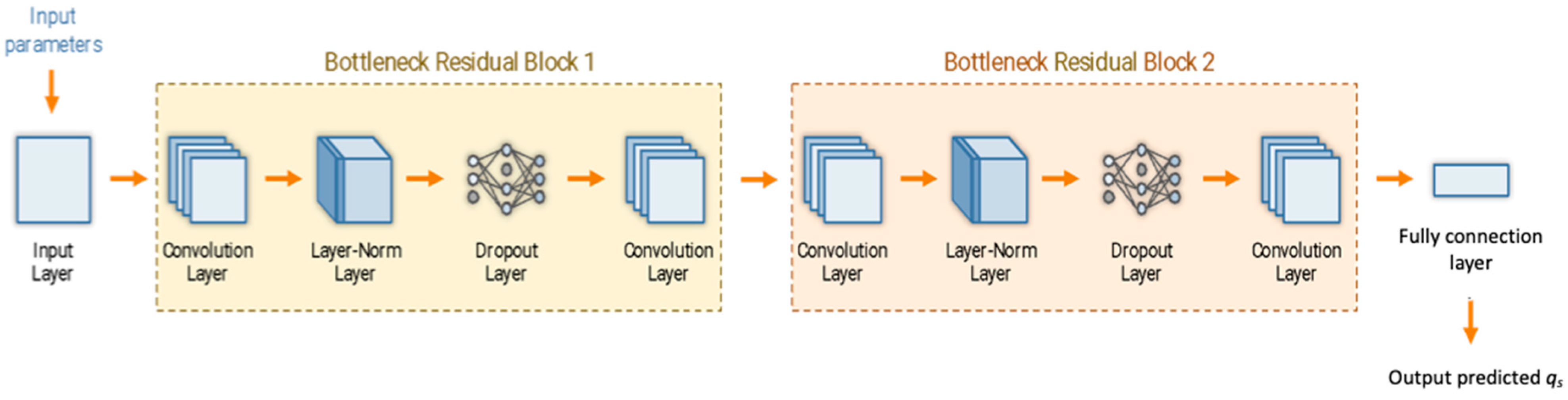
3.1. Model Description
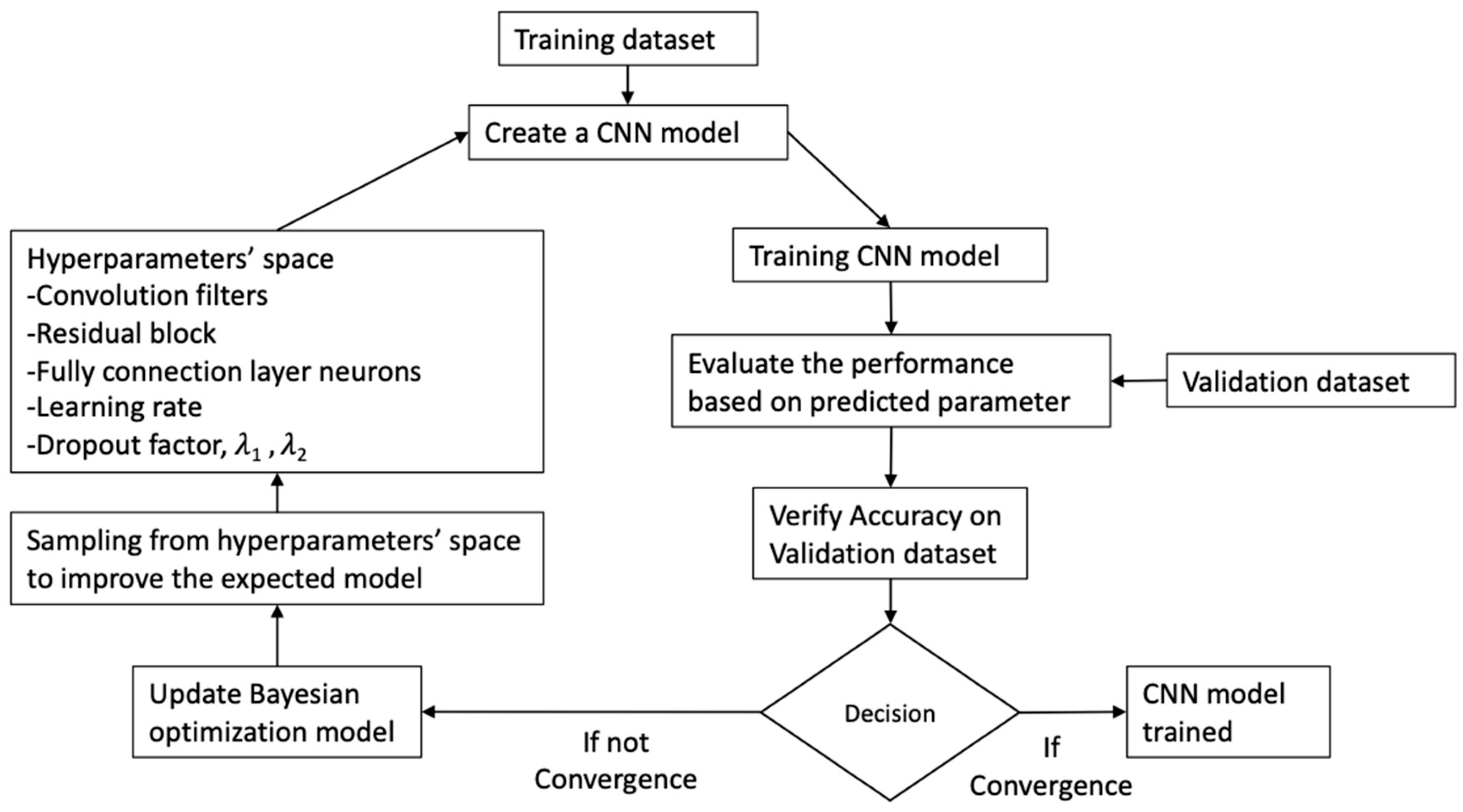
3.2. CNN Training with Hyperparameter Optimization
4. Results and Discussion
4.1. Training Setup
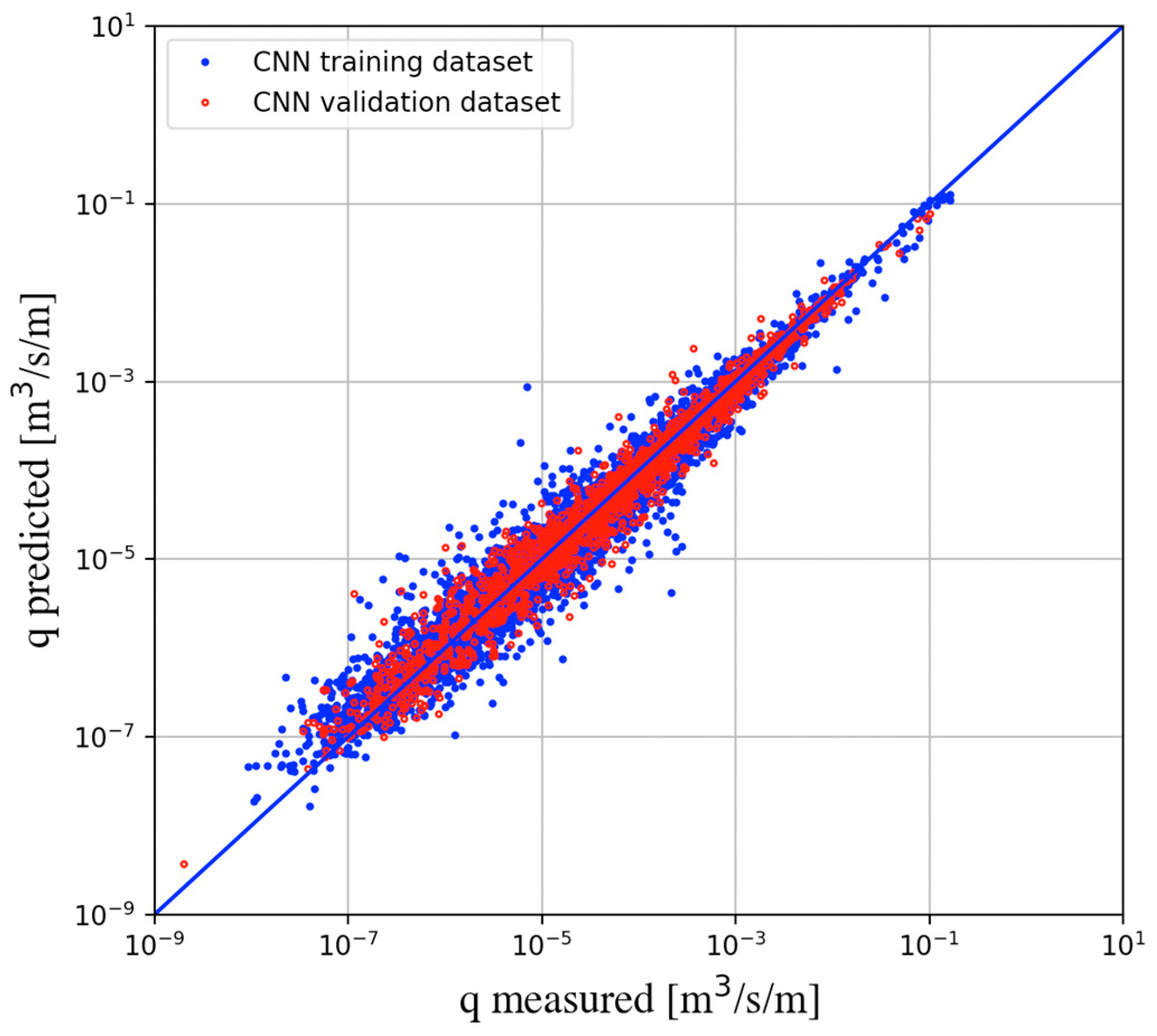
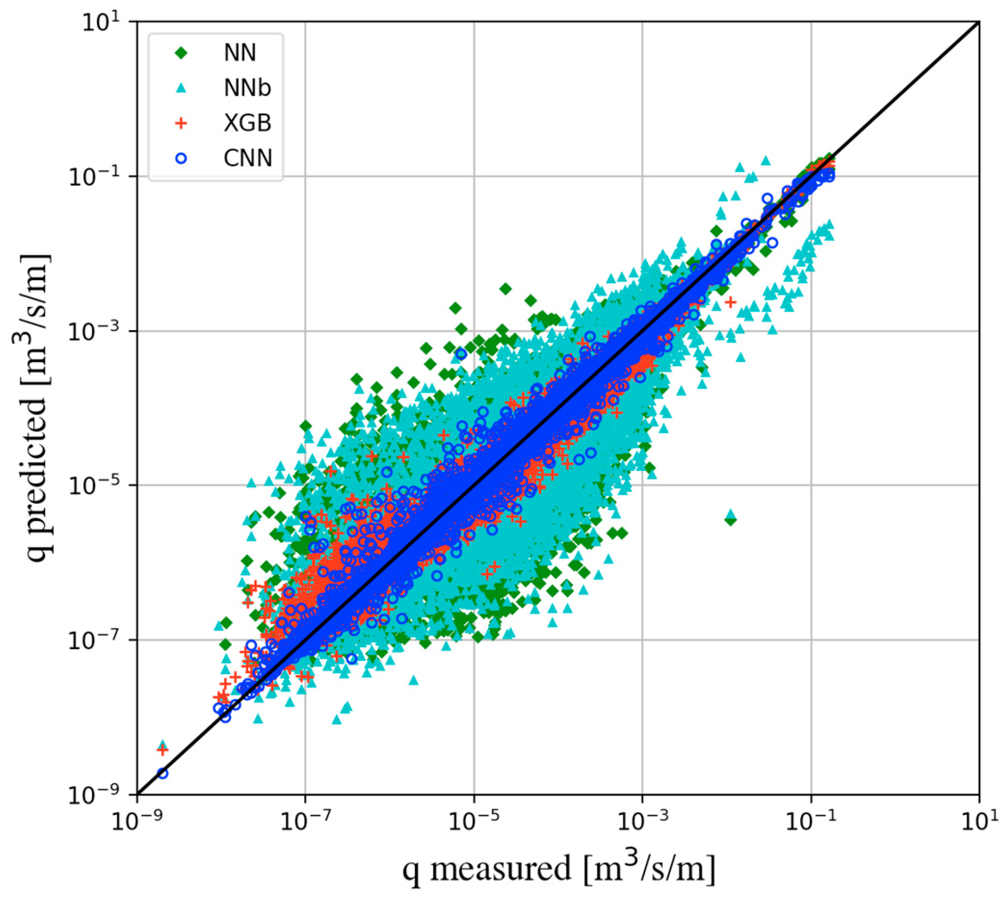
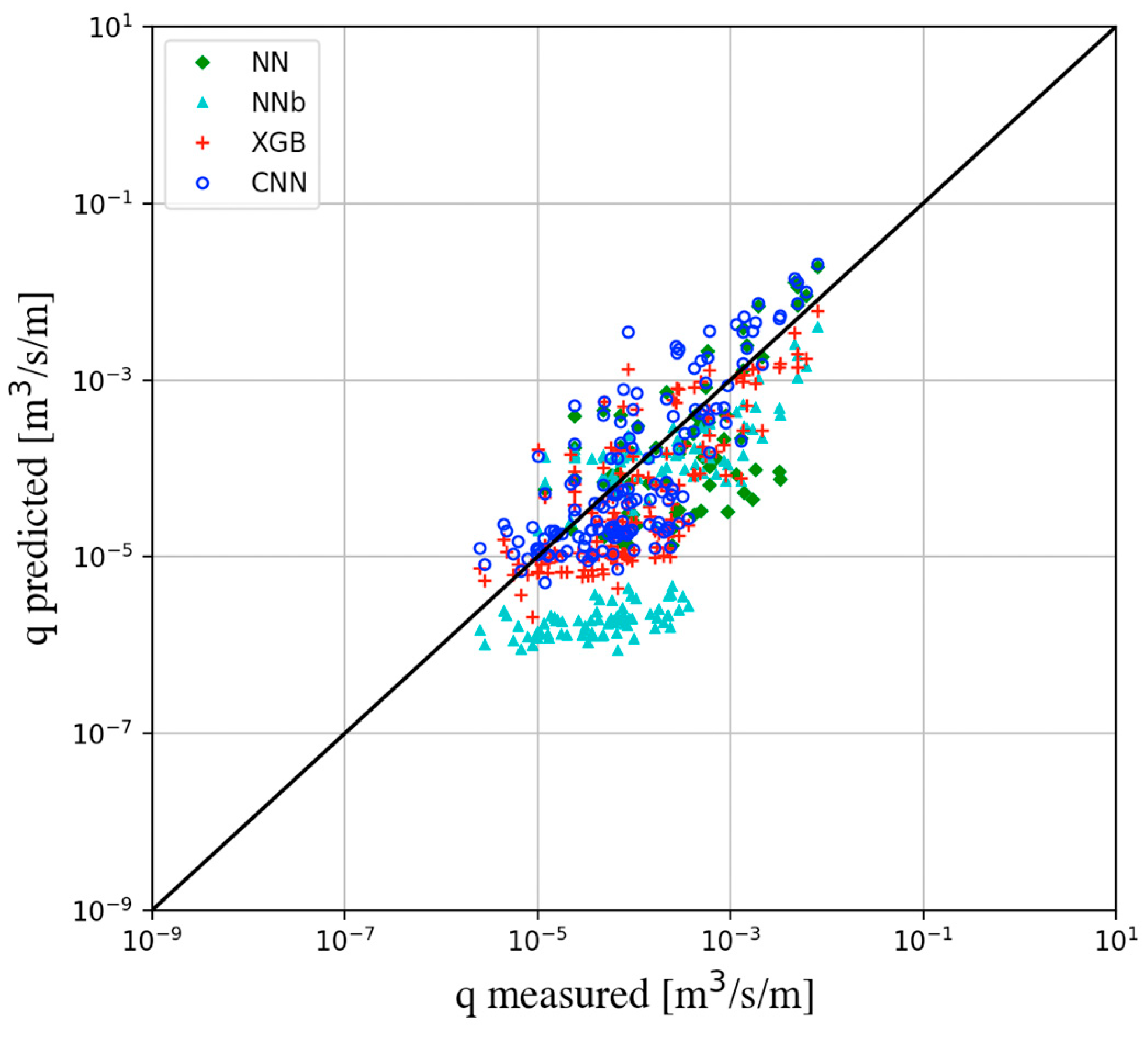
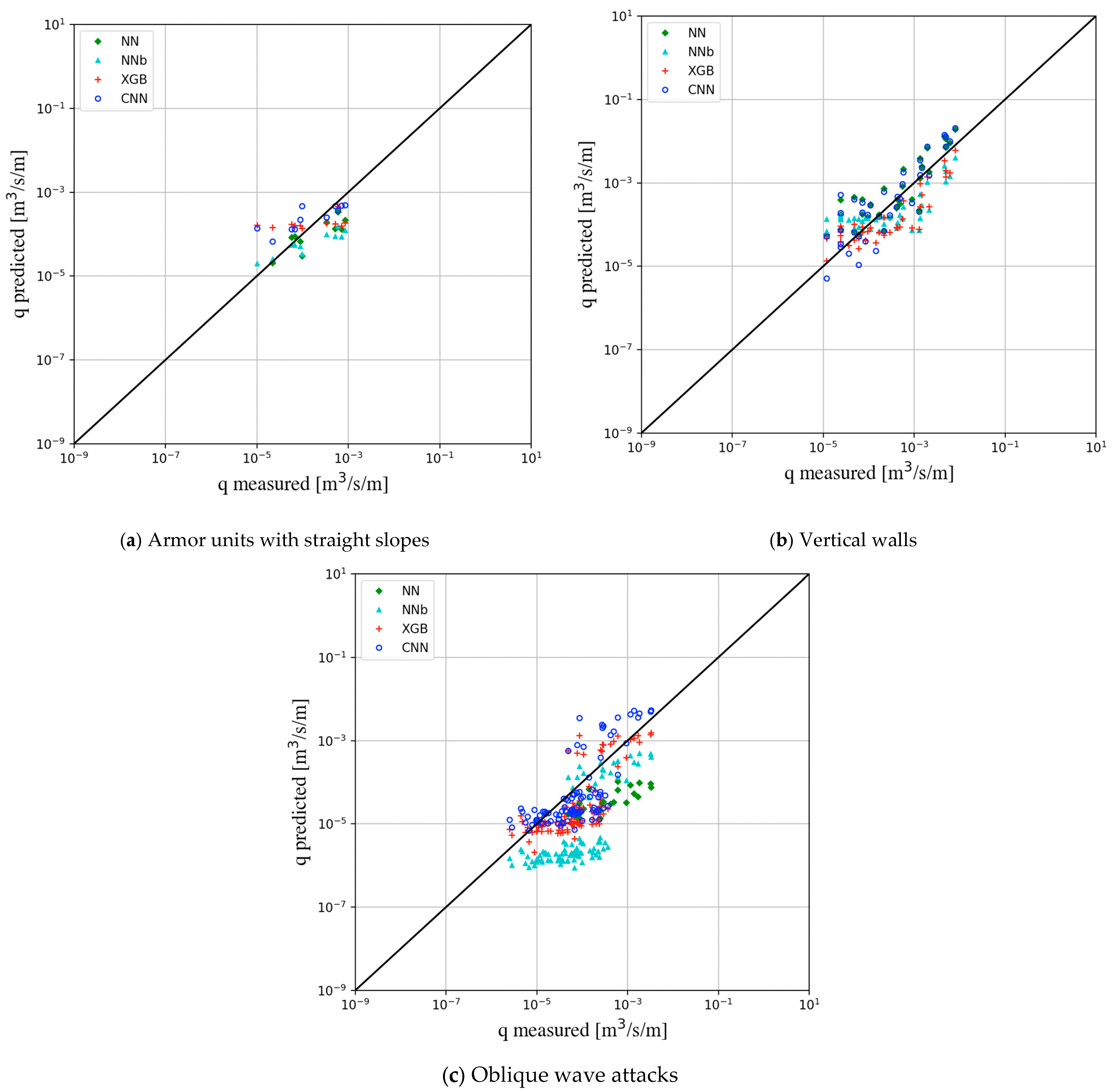
4.2. Verification on the Overtopping Database
4.3. Testing/Prediction Using Prototype Overtopping Dataset
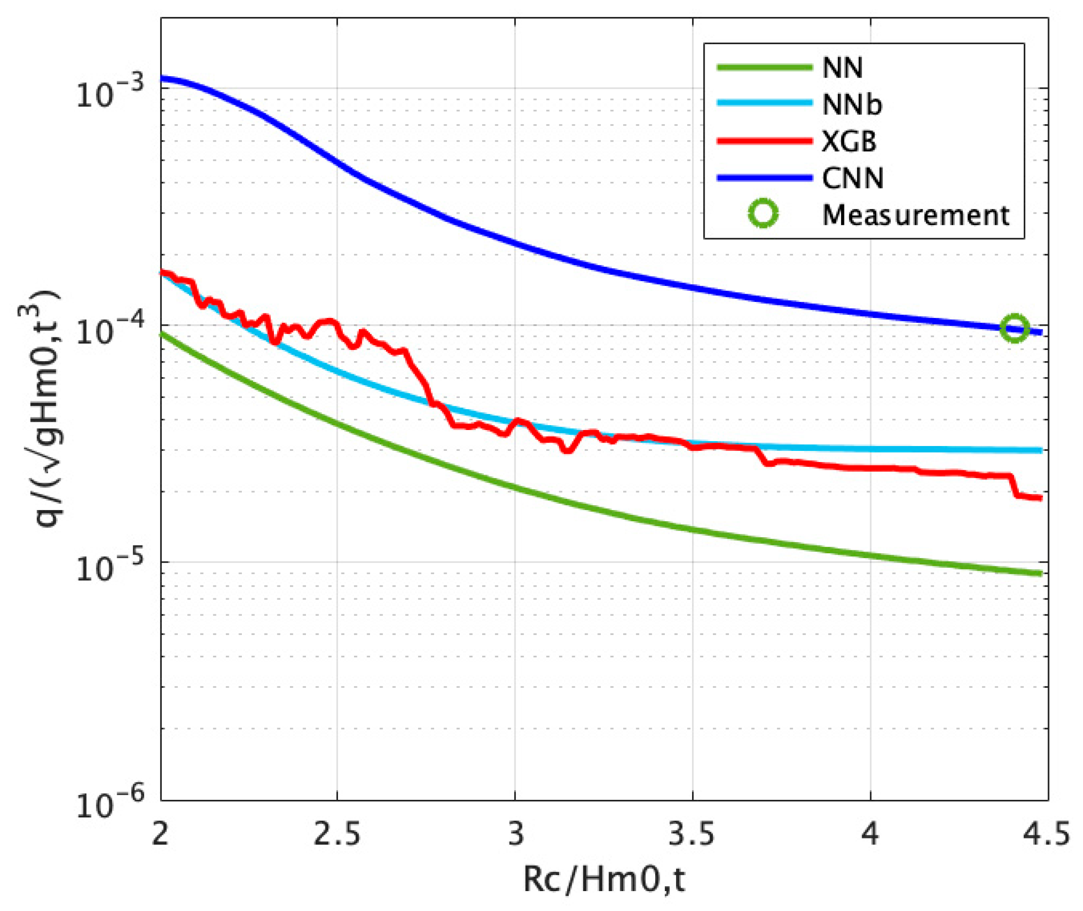
4.4. Application of CNN for Prototype Various Crest Freeboards
5. Conclusions
Supplementary Materials
Author Contributions
Funding
Data Availability Statement
Acknowledgments
Conflicts of Interest
References
- Troch, P.; Geeraerts, J.; Van de Walle, B.; De Rouck, J.; Van Damme, L.; Allsop, W.; Franco, L. Full-scale wave-overtopping measurements on the Zeebrugge rubble mound breakwater. Coast. Eng. 2004, 51, 609–628. [Google Scholar] [CrossRef]
- Briganti, R.; Bellotti, G.; Franco, L.; De Rouck, J.; Geeraerts, J. Field measurements of wave overtopping at the rubble mound breakwater of Rome–Ostia yacht harbour. Coast. Eng. 2005, 52, 1155–1174. [Google Scholar] [CrossRef]
- Cáceres, I.; Sánchez-Arcilla, A.; Zanuttigh, B.; Lamberti, A.; Franco, L. Wave overtopping and induced currents at emergent low crested structures. Coast. Eng. 2005, 52, 931–947. [Google Scholar] [CrossRef]
- van Gent, M.R.A.; van den Boogaard, H.F.P.; Pozueta, B.; Medina, J.R. Neural network modelling of wave overtopping at coastal structures. Coast. Eng. 2007, 54, 586–593. [Google Scholar] [CrossRef]
- Losada, I.J.; Lara, J.L.; Guanche, R.; Gonzalez-Ondina, J.M. Numerical analysis of wave overtopping of rubble mound breakwaters. Coast. Eng. 2008, 55, 47–62. [Google Scholar] [CrossRef]
- Reeve, D.E.; Soliman, A.; Lin, P.Z. Numerical study of combined overflow and wave overtopping over a smooth impermeable seawall. Coast. Eng. 2008, 55, 155–166. [Google Scholar] [CrossRef]
- Verhaeghe, H.; De Rouck, J.; van der Meer, J. Combined classifier–quantifier model: A 2-phases neural model for prediction of wave overtopping at coastal structures. Coast. Eng. 2008, 55, 357–374. [Google Scholar] [CrossRef]
- De Rouck, J.; Verhaeghe, H.; Geeraerts, J. Crest level assessment of coastal structures—General overview. Coast. Eng. 2009, 56, 99–107. [Google Scholar] [CrossRef]
- EurOtop. Manual on Wave Overtopping of Sea Defences and Related Structures. An Overtopping Manual Largely Based on European Research, but for Worldwide Application; Van der Meer, J.W.; Allsop, N.W.H.; Bruce, T.; De Rouck, J.; Kortenhaus, A.; Pullen, T.; Schüttrumpf, H.; Troch, P.; Zanuttigh, B.: 2018. Available online: www.overtopping-manual.com (accessed on 1 November 2019).
- van der Meer, J.W.; Verhaeghe, H.; Steendam, G.J. The new wave overtopping database for coastal structures. Coast. Eng. 2009, 56, 108–120. [Google Scholar] [CrossRef]
- Zanuttigh, B.; Formentin, S.M.; van der Meer, J.W. Prediction of extreme and tolerable wave overtopping discharges through an advanced neural network. Ocean Eng. 2016, 127, 7–22. [Google Scholar] [CrossRef]
- den Bieman, J.P.; van Gent, M.R.A.; van den Boogaard, H.F.P. Wave overtopping predictions using an advanced machine learning technique. Coast. Eng. 2021, 166, 103830. [Google Scholar] [CrossRef]
- Heaton, J. Ian Goodfellow, Yoshua Bengio, Aaron Courville. Deep learning. Genet. Program. Evolvable Mach. 2018, 19, 305–307. [Google Scholar] [CrossRef]
- Hochreiter, S.; Schmidhuber, J. Long short-term memory. Neural. Comput. 1997, 9, 1735–1780. [Google Scholar] [CrossRef]
- Formentin, S.M.; Zanuttigh, B.; van der Meer, J.W. The New EurOtop Neural Network Tool for an Improved Prediction of Wave Overtopping. In ICE Coasts, Marine Structures and Breakwaters; ICE Publishing: Leeds, UK, 2017. [Google Scholar]
- Formentin, S.M.; Zanuttigh, B.; van der Meer, J.W. A Neural Network Tool for Predicting Wave Reflection, Overtopping and Transmission. Coast. Eng. J. 2018, 59, 1750006-1–1750006-31. [Google Scholar] [CrossRef]
- Ba, J.L.; Kiros, J.R.; Hinton, G.E. Layer Normalization. arXiv 2016, arXiv:1909.11855. [Google Scholar]
- Srivastava, N.; Hinton, G.; Krizhevsky, A.; Sutskever, I.; Salakhutdinov, R. Dropout: A Simple Way to Prevent Neural Networks from Overfitting. J. Mach. Learn. Res. 2014, 15, 1929–1958. [Google Scholar]
- Wang, F.; Jiang, M.; Qian, C.; Yang, S.; Li, C.; Zhang, H.; Wang, X.; Tang, X. Residual attention network for image classification. In Proceedings of the IEEE Conference on Computer Vision and Pattern Recognition, Honolulu, HI, USA, 21–26 July 2017; pp. 3156–3164. [Google Scholar]
- Ying, X. An Overview of Overfitting and its Solutions. J. Phys. Conf. Ser. 2019, 1168, 022022. [Google Scholar] [CrossRef]
- Isabona, J.; Imoize, A.L.; Kim, Y. Machine Learning-Based Boosted Regression Ensemble Combined with Hyperparameter Tuning for Optimal Adaptive Learning. Sensors 2022, 22, 3776. [Google Scholar] [CrossRef]
- Sóbester, A.; Leary, S.J.; Keane, A.J. On the Design of Optimization Strategies Based on Global Response Surface Approximation Models. J. Glob. Optim. 2005, 33, 31–59. [Google Scholar] [CrossRef]
- Friedman, J.H. Greedy function approximation: A gradient boosting machine. Ann. Stat. 2001, 29, 1189–1232. [Google Scholar] [CrossRef]
- Mueller, J.; Jaakkola, T. Principal Differences Analysis: Interpretable Characterization of Differences between Distributions. arXiv 2015, arXiv:1510.08956. [Google Scholar]
- Diederik, P.; Kingma, J.B. Adam: A Method for Stochastic Optimization. In Proceedings of the 3rd International Conference for Learning Representations, San Diego, CA, USA, 7–9 May 2015. [Google Scholar]
- Scikit-Optimize. Sequential Model-Based Optimization in Python. Available online: https://scikit-optimize.github.io/ (accessed on 1 May 2023).
- Abadi, M.; Barham, P.; Chen, J.; Chen, Z.; Davis, A.; Dean, J.; Devin, M.; Ghemawat, S.; Irving, G.; Isard, M. Tensorflow: A system for large-scale machine learning. In Proceedings of the 12th USENIX Symposium on Operating Systems Design and Implementation, Savannah, GA, USA, 2–4 November 2016; pp. 265–283. [Google Scholar]
- Geeraerts, J.; Boone, C. Report on Full Scale Measurements Zeebrugge, 2nd Full Winter Season; Ghent University: Gent, Belgium, 2004. [Google Scholar]
- Franco, L.; Briganti, R.; Bellotti, G. Report on Full Scale Measurements, Ostia, 2nd Full Winter Season; Modimar: Rome, Italy, 2004. [Google Scholar]
- Pullen, T. Final Report on Laboratory Measurements, Samphire Hoe; HR Wallingford: Wallingford, UK, 2004. [Google Scholar]


| # | Parameters | Definition of the Parameters | |
|---|---|---|---|
| 1 | Hydraulic parameters of waves | Hm0,t/Lm−1,0,t | Wave steepness at the structure toe |
| 2 | h/Lm−1,0,t | Relative water depth at the structure toe | |
| 3 | Wave obliquity | ||
| 4 | Structure parameters | ht/Hm0,t | Relative submergence of the toe structure |
| 5 | Bt/Lm−1,0,t | Relative width of the toe structure | |
| 6 | Cotangent of the structure slope below the berm | ||
| 7 | Cotangent of the structure slope above the berm | ||
| 8 | Roughness factor for | ||
| 9 | Roughness factor for | ||
| 10 | Dd/Hm0,t | Relative size of the armor elements along | |
| 11 | Du/Hm0,t | Relative size of the armor elements along | |
| 12 | Ac/Hm0,t | Relative crest freeboard of armor structure | |
| 13 | Rc/Hm0,t | Relative crest freeboard of wall | |
| 14 | Gc/Lm−1,0,t | Relative crest width of armor structure | |
| 15 | B/Lm−1,0,t | Relative berm width | |
| 16 | hb/Lm−1,0,t | Relative berm submergence | |
| 1 | Predicted parameter | qs | Normalized wave overtopping discharge per unit width |
| Hyperparameter Name | Values | Definition of the Hyperparameter |
|---|---|---|
| Convolution_filters | [16, 24, 32, 64, 128, 256 *] | Number of filters in each convolution layer |
| Residual_block | [1, 2 *] | Number of residual block |
| Fully_connection_layer_neurons | [32, 64, 128 *, 256, 512] | Neurons in a fully connected layer |
| Learning_rate | [0.0001 *, 0.0002, …, 0.1] | Given range of learning rate for CNN training |
| Dropout_rate | [0.1, 0.2, …0.7 *, 0.8, 0.9], | Determines the probability of a neuron being dropped out |
| λ1 | [0.5, 0.6, …, 1.0 *] | Given weights of RMSE term of L |
| λ2 | [0.1, 0.2,…, 0.5 *, …, 1.0] | Given weights for constraint term of L |
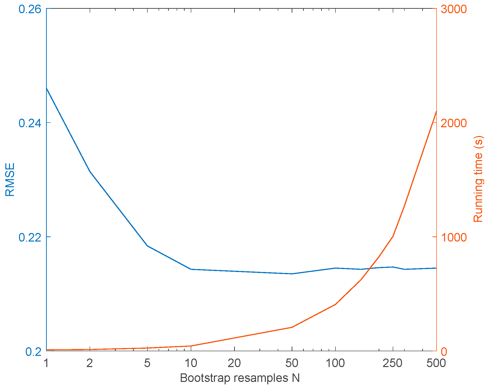
| Dataset (Size) | Bootstrap Resamples | ||
|---|---|---|---|
| N = 1 | N = 10 | N = 500 | |
| Training data (6922) | 0.238 | 0.230 | 0.225 |
| Validation data (1731) | 0.246 | 0.214 | 0.215 |
| Dataset (Size) | Model | RMSE | CC | R2 |
|---|---|---|---|---|
| Entire core data (8653) | NN | 0.654 | 0.869 | 0.756 |
| NNb | 0.639 | 0.858 | 0.736 | |
| XGB | 0.199 | 0.990 | 0.981 | |
| CNN | 0.112 | 0.996 | 0.991 | |
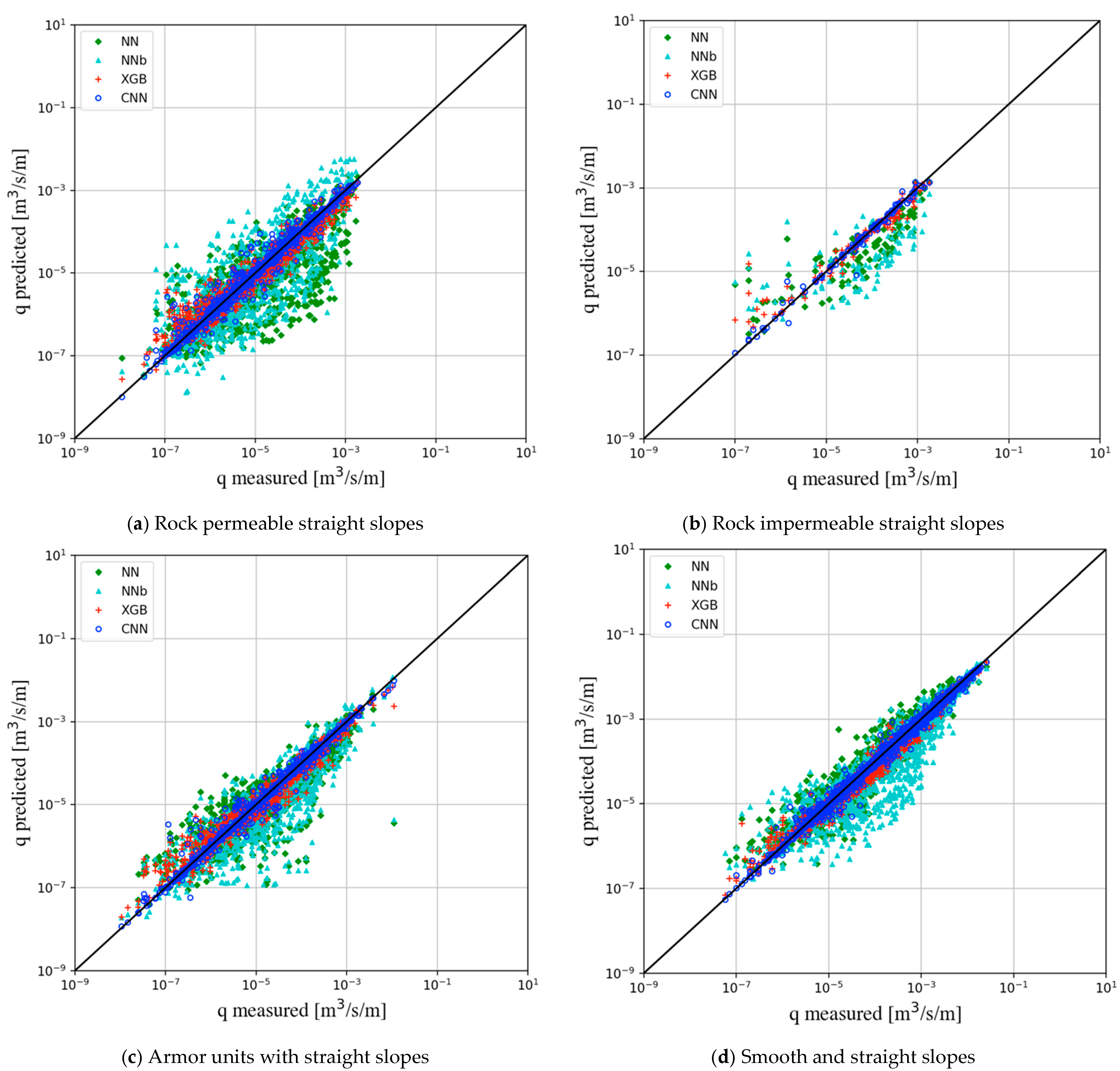
| A: rock permeable straight slopes (1131) | NN | 0.702 | 0.768 | 0.590 |
| NNb | 0.687 | 0.791 | 0.625 | |
| XGB | 0.247 | 0.977 | 0.955 | |
| CNN | 0.153 | 0.989 | 0.978 | |
| B: rock impermeable straight slopes (104) | NN | 0.624 | 0.864 | 0.747 |
| NNb | 0.823 | 0.710 | 0.504 | |
| XGB | 0.349 | 0.984 | 0.968 | |
| CNN | 0.136 | 0.994 | 0.989 | |
| C: armor units with straight slopes (934) | NN | 0.506 | 0.872 | 0.760 |
| NNb | 0.583 | 0.858 | 0.737 | |
| XGB | 0.219 | 0.983 | 0.966 | |
| CNN | 0.118 | 0.991 | 0.983 | |
| D: smooth and straight slopes (2069) | NN | 0.480 | 0.972 | 0.946 |
| NNb | 0.380 | 0.943 | 0.889 | |
| XGB | 0.120 | 0.996 | 0.991 | |
| CNN | 0.086 | 0.997 | 0.994 | |
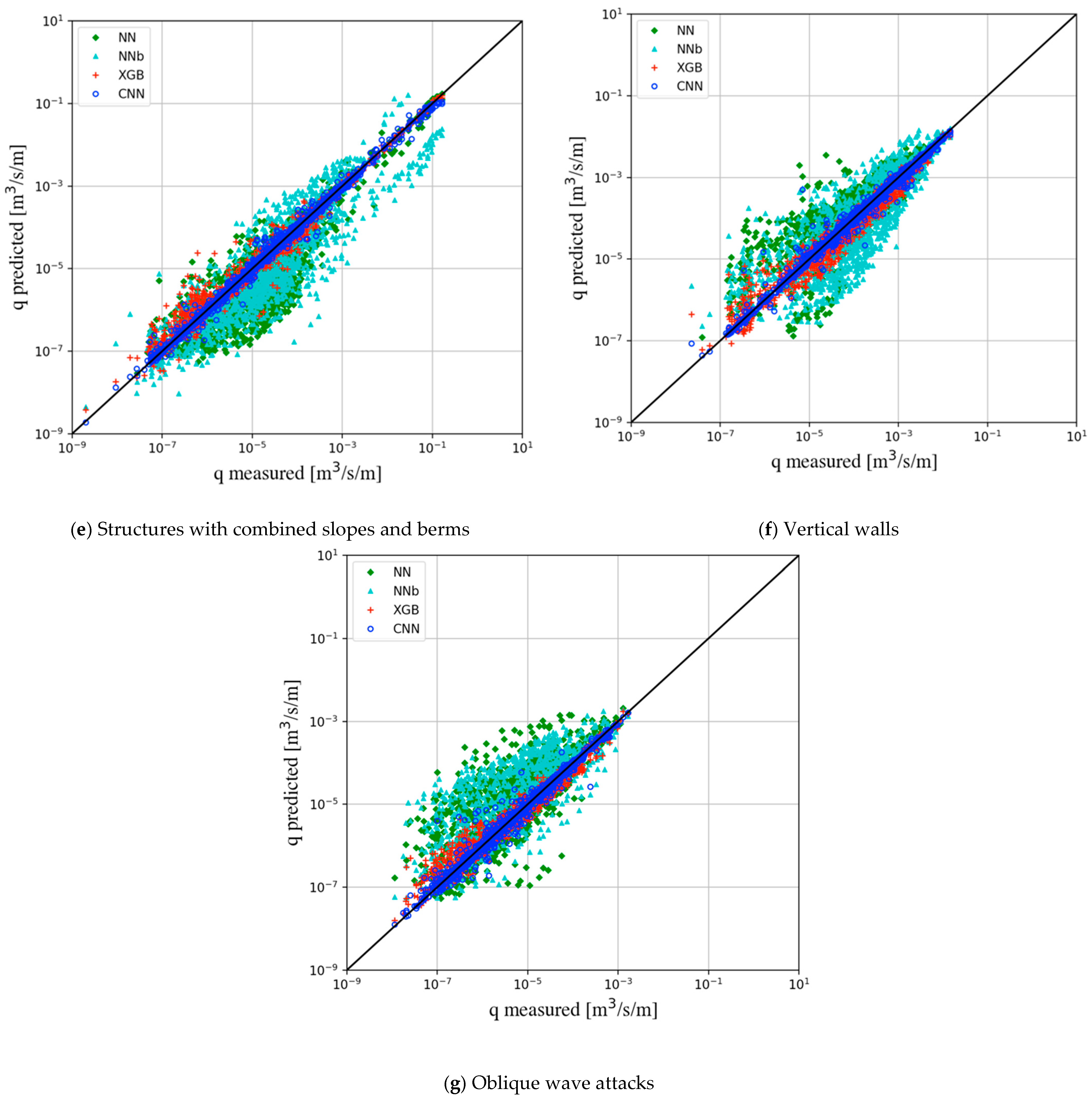
| E: structures with combined slopes and berms (1631) | NN | 0.784 | 0.838 | 0.703 |
| NNb | 0.670 | 0.877 | 0.770 | |
| XGB | 0.204 | 0.987 | 0.975 | |
| CNN | 0.093 | 0.997 | 0.993 | |
| F: vertical walls (1677) | NN | 0.685 | 0.863 | 0.745 |
| NNb | 0.704 | 0.845 | 0.714 | |
| XGB | 0.206 | 0.988 | 0.977 | |
| CNN | 0.110 | 0.994 | 0.988 | |
| G: oblique wave attacks (1107) | NN | 0.760 | 0.777 | 0.603 |
| NNb | 0.872 | 0.772 | 0.595 | |
| XGB | 0.228 | 0.983 | 0.965 | |
| CNN | 0.128 | 0.989 | 0.978 |
| Dataset (Size) | Model | RMSE | CC | R2 |
|---|---|---|---|---|
| All testing data (150) | NN* | 0.936 | 0.874 | 0.764 |
| NNb | 1.218 | 0.895 | 0.802 | |
| XGB | 0.657 | 0.868 | 0.753 | |
| CNN | 0.555 | 0.932 | 0.868 |
| Parameter | Value | Parameter | Value | Parameter | Value |
|---|---|---|---|---|---|
| Hmo,t [m] | 1.67 | Rc [m] | 3.34 to 7.50 | Dd [m] | 0.60 |
| hb [m] | 1.03 | Ac [m] | 3.34 | Du [m] | 0.00 |
| ht [m] | 3.28 | Gc [m] | 1.00 | 0.55 | |
| h [m] | 3.28 | B [m] | 8.00 | 1.00 | |
| Lm−1,0,t [m] | 59.39 | cotαd | 1.00 | β [°] | 14 |
| Bt [m] | 0.00 | cotαu | 0.00 |
Disclaimer/Publisher’s Note: The statements, opinions and data contained in all publications are solely those of the individual author(s) and contributor(s) and not of MDPI and/or the editor(s). MDPI and/or the editor(s) disclaim responsibility for any injury to people or property resulting from any ideas, methods, instructions or products referred to in the content. |
© 2023 by the authors. Licensee MDPI, Basel, Switzerland. This article is an open access article distributed under the terms and conditions of the Creative Commons Attribution (CC BY) license (https://creativecommons.org/licenses/by/4.0/).
Share and Cite
Tsai, Y.-T.; Tsai, C.-P. Predictions of Wave Overtopping Using Deep Learning Neural Networks. J. Mar. Sci. Eng. 2023, 11, 1925. https://doi.org/10.3390/jmse11101925
Tsai Y-T, Tsai C-P. Predictions of Wave Overtopping Using Deep Learning Neural Networks. Journal of Marine Science and Engineering. 2023; 11(10):1925. https://doi.org/10.3390/jmse11101925
Chicago/Turabian StyleTsai, Yu-Ting, and Ching-Piao Tsai. 2023. "Predictions of Wave Overtopping Using Deep Learning Neural Networks" Journal of Marine Science and Engineering 11, no. 10: 1925. https://doi.org/10.3390/jmse11101925