Transfer Learning with Deep Neural Network toward the Prediction of Wake Flow Characteristics of Containerships

Abstract

In this study, deep neural network (DNN) and transfer learning (TL) techniques were employed to predict the viscous resistance and wake distribution based on the positions of flow control fins (FCFs) applied to containerships of various sizes. Both methods utilized data collected through computational fluid dynamics (CFD) analysis. The position of the flow control fin (FCF) and hull form information were utilized as input data, and the output data included viscous resistance coefficients and components of propeller axial velocity. The base DNN model was trained and validated using a source dataset from a 1000 TEU containership. The grid search cross-validation technique was employed to optimize the hyperparameters of the base DNN model. Then, transfer learning was applied to predict the viscous resistance and wake distribution for containerships of varying sizes. To enhance the accuracy of feature prediction with a limited amount of data, learning rate optimization was conducted. Transfer learning involves retraining and reconfiguring the base DNN model, and the accuracy was verified based on the fine-tuning method of the learning model. The results of this study can provide hull designers for containerships with performance evaluation information by predicting wake distribution, without relying on CFD analysis.

1. Introduction

The severity of environmental issues resulting from industrial development has become a global concern, spanning various sectors, including the shipbuilding industry. As a result, various related regulations are being formulated or strengthened. In 2018, the International Maritime Organization (IMO) announced a strategy to reduce the total greenhouse gas emissions from ships by 50% and the Carbon Intensity Indicator (CII) by 70% by the year 2050, compared to the levels in 2008. As one of the initial strategies, the implementation of the EEXI (Energy Efficiency Existing Ship Index) and the CII (Carbon Intensity Index) rating system is already in place. This represents a significant strengthening of energy efficiency regulations for existing ships. The efforts to meet EEXI compliance and achieve higher CII ratings are tasks assigned to the existing ships. Among several strategies for this purpose, one approach is to enhance resistance performance, and this can be achieved through the application of energy-saving devices (ESDs). The application of ESDs involves installing relatively small-scale devices that can lead to significant effects. Because of this, ESDs are utilized in various ways, not only for existing ships but also for the design of new ships.

Samsung Heavy Industries registered a patent in 2007 [1] for SAVER (Samsung Vibration and Energy Reduction) Fins. These FCFs are designed to control the inflow fluid dynamics above and below the propeller of ships, to improve pressure resistance and reduce vibrations. Lee et al. [2] applied the SAVER Fins in combination with a rudder bulb to a 35 K DWT bulk carrier and confirmed a power-saving effect of 7.4% through model tests and sea trials. Kim et al. [3] attached vertical plates to the stern of a 24 K tanker and confirmed improvements in resistance performance and wake distribution through computational fluid dynamics (CFD) analysis. Lee et al. [4] investigated the changes in resistance performance and wake characteristics based on the position of FCF and the angle with the streamline using CFD analysis, focusing on an 80 K bulk carrier. Recently, Park et al. [5] demonstrated through model tests and CFD that FCF can reduce the total resistance of a 6.5 K DWT tanker by 4.3%. Many studies have been conducted on FCF design, and the effects of FCF are predominantly verified through model tests and CFD simulations. Furthermore, research has advanced to predict or optimize the effects of FCF using artificial intelligence techniques as a basis. A neural network was trained based on hull form data and then used to predict the wake distribution [6]. Another example is Kim and Moon [7], who used a neuro-fuzzy technique to predict wake distribution. Wie and Kim [8] carried out an optimal FCF design for the Kriso 300 K VLCC using a genetic algorithm (GA) and NLPQL (non-linear programming by quadratic Lagrangian). Liu et al. [9] built an approximate fluid dynamics model for ships based on Kriging and Co-Kriging models. This model has been successfully utilized for cost-effective resistance optimization and flow field predictions. Feng et al. [10] employed a surrogate model based on Support vector regression (SVR) to improve the resistance and wake field of offshore aquaculture vessel hull form. Machine learning is being applied in various fields within the shipbuilding industry, not just for appendage design like FCF. Su et al. [11] proposed a real-time ship vertical acceleration prediction algorithm based on long short-term memory (LSTM) and gated recurrent unit (GRU) models. Mittendorf et al. [12] used nonlinear regression algorithms (random forests, extreme gradient boosting machines, and multilayer perceptron) to predict the added wave resistance of ships in head-to-beam wave conditions. Lin et al. [13] developed an efficient anti-rolling controller using the deep deterministic policy gradient (DDPG) algorithm based on deep reinforcement learning (DRL).

In the previous paper by the authors of [14], optimal FCF design was performed for a small containership using two strategies: neural network-based machine learning and optimization techniques. The advantage of machine learning (ML) over CFD simulation is the computational efficiency. In the previous study regarding the optimal design of FCF for a 1000 TEU containership, the authors reported the enormous saving of computational time spent for the multi-objective optimization based on genetic algorithm (GA). Specifically, the entire GA required 20,000 simulations which would have taken approximately 10,000 h. However, the DNN-based prediction took only 4.5 min.

The objective of this current study is to extend such advantage of machine learning to more containerships, not just for a single containership. This was completed by adopting transfer learning (TL) to generalize the existing deep neural network (DNN) for a 1000 TEU containership to predict the wake field prediction for various containerships. It is well known that the TL is particularly effective when the data for the different tasks are not enough. Initially, a deep neural network (DNN) model is employed to predict the performance of a single containership with a substantial dataset available. The hyperparameters required for model configuration are optimized using grid search cross-validation. Subsequently, based on the base DNN model, transfer learning (TL) is utilized to predict performance for the remaining containerships with limited data of 150 datasets for two containerships. In this study, a small number of hull forms are applied to transfer learning to predict the fluid dynamic performance based on the FCF position. This can be utilized as foundational research for expanding the applicability of fluid dynamic performance prediction techniques to containerships of various sizes and even to different types of vessels. Additionally, it is considered that the combination of transfer learning-based performance prediction and appropriate optimization algorithms can be extended to the FCF design of containerships of various sizes.

The paper organization is as follows: Section 2 presents the target ships and FCF specifications and formulates the numerical methods to prepare for the data; Section 3 describes the theoretical background of deep neural networks and transfer learning, detailing the specific processes applied in this study. Subsequently, Section 4 presents the performance prediction results for containerships of various sizes. Finally, Section 5 discusses the main conclusions and findings.

2. Problem Descriptions

2.1. Target Ship and Flow Control Fins

The base DNN used for predicting wake distribution and resistance is trained using data from the author’s previous paper. A relatively substantial amount of data used for training the DNN model comes from a 1000 TEU containership constructed by Daesun Shipbuilding & Engineering Co., Ltd. This was associated with the presence of reliable CFD data. A model with a scale ratio $\lambda =30.56$ was selected for numerical simulation. The data used for the transfer learning model consists of different sized vessels: 2500 TEU and 3600 TEU (KCS; KRISO Containership) containerships. For these ships, models with each scale ratio of $\lambda =27.2$ and $\lambda =31.6$ were considered. The principal dimensions of target hulls and propellers are given in

Table 1. Principal particulars of 1000 TEU containership.

Class	Designation	Symbol (Unit)	Full-Scale Ship
1000 TEU	Length bet. Perpendicular	$L_{PP}$ (m)	137.5
	Breadth	$B$ (m)	23.6
	Draft	$T$ (m)	7.4
	Block coefficient	$C_B$	0.595
	Propeller diameter	$DIA$ (m)	5.5
2500 TEU	Length bet. Perpendicular	$L_{PP}$ (m)	185.0
	Breadth	$B$ (m)	32.26
	Draft	$T$ (m)	10.0
	Block coefficient	$C_B$	0.640
	Propeller diameter	$DIA$ (m)	6.8
3600 TEU	Length bet. Perpendicular	$L_{PP}$ (m)	230.0
	Breadth	$B$ (m)	32.2
	Draft	$T$ (m)	10.8
	Block coefficient	$C_B$	0.651
	Propeller diameter	$DIA$ (m)	7.9

. Figure 1 presents the three-dimensional views of target hull forms and propellers.

The flow control fin (FCF) used in this study is rectangular in shape with two rounded corners (see Figure 2). The dimensions of full-scale FCF were 1.30 m long, 0.37 m high, and 0.03 m thick. When normalized by the propeller diameter $D$, these correspond to $0.236D$ (length) × $0.0673D$ (height) × $0.00545D$ (thickness). Generally, FCFs are attached in pair(s) at the same locations on the port and starboard sides. The design variables for the FCF are the longitudinal and vertical positions of the FCF, inclination angle, and hull form information. Here, the position of the FCF is located at the midpoint of the baseline, and the angle of inclination refers to the angle between the FCF baseline and the ship baseline. The hull form information applies the derivatives representing the gradient of each tangent at the midpoint of the FCF in the directions of the station, waterline, and buttock line. In more detail, when the derivative is small in the station direction, it indicates that when observing the hull form in the body plan, the shape resembles a V type. Similarly, when the derivatives are small in the waterline and buttock line directions, they represent hull form that changes smoothly in the half-breadth and shear plan, respectively.

Indeed, even within the same type of vessel, differences in main particulars, hull form, and the position of the FCF can result in variations in the characteristics of the propeller inflow velocity distribution. Figure 3 illustrates the distribution of the viscous resistance coefficient and the standard deviation of axial velocity distribution based on derivatives in the waterline and buttock line directions. The orange symbols represent the viscosity resistance coefficients and standard deviation for 1000 TEU, the green symbols for 2500 TEU, and the blue symbols for 3600 TEU. Transfer learning was employed to predict values with varying characteristics across different ship sizes.

2.2. CFD Simulation to Obtain Training Data

In this study, 693 datasets were prepared by the CFD analysis to train, validate, and test the base DNN model. Each set of data corresponded to a combination of design parameters, including 11 longitudinal positions $\left(3.0\le x/St.\le 4.0, ∆x/St.=0.1\right)$ $\times$ vertical positions $\left(0.135\le z/T\le 0.405, ∆z/T=0.0135\right)$ $\times 3$ inclination angles $(\alpha =19°, 20°, 21°)$. Here, $St.$ refers to the station length, which is 1/20 of the length between perpendicular $L_{PP}$. Around 150 target datasets for 2500 TEU and 3600 TEU were obtained through CFD analysis for transfer learning. The target datasets were randomly selected within the same longitudinal and vertical position ranges as the source datasets. Similarly, the inclination angles were also randomly specified.

It is necessary to emphasize the importance of automation in such preprocessing steps as modeling and mesh generation, as it significantly enhances the overall computational efficiency for the entire set of 843 simulation cases. The processes including three-dimensional modeling of hull forms with varying FCF positions, mesh generation, and creation of CFD setups was carried out using OptHull^® software, a professional hull form design software. Then, the commercial CFD S/W STAR-CCM+ was configured and the numerical analysis was automatically controlled by an in-house JavaScript code. By using a 140 CPU (Intel Xeon 2.6 GHz)-parallel computing cluster, approximately 419 h were required to complete the preparation of data for the 843 simulations.

2.2.1. Governing Equations

The STAR-CCM+ v.15.06 was used for the CFD analysis of the flow around the ship. The governing equations consist of the continuity equation for mass conservation and the Reynolds-averaged Navier–Stokes (RANS) equations for momentum and energy conservation. These equations are given in the following tensor notation:

$$\frac{\partial U_i}{\partial x_i}=0$$

(1)

$$\frac{\partial U_i}{\partial t}+\rho U_l\frac{\partial U_i}{\partial x_l}=-\frac{\partial p}{\partial x_i}+\frac{\partial }{\partial x_l}\left(\mu \frac{\partial U_i}{\partial x_l}-\rho \overline{u_i{u}_l}\right)+\rho g_i$$

(2)

where $U_i=\left(U,V,W\right)$ is the velocity component in $x_i=\left(x,y,z\right)$ direction, while $p, \rho , \mu ,-\overline{u_i{u}_l}$ and $g_i$ are the static pressure, fluid density, absolute viscosity of fluid, Reynolds stress, and gravitational acceleration in the $x_i$-direction, respectively.

The Reynolds stress turbulent model, being excellent in resolving bilge vortex and capable of high-accuracy prediction of flow around the ship [15], was employed in the numerical analysis. The transport equation for the Reynolds stress is described as follows:

$$\frac{D\overline{u_i^{\prime }{u}_j^{\prime }}}{Dt}=D_{ij}+G_{ij}-\frac{2}{3}{\delta }_{ij}\epsilon +PS$$

(3)

where ${\delta }_{ij}$ is the Kronecker delta and $D_{ij}$, $G_{ij}$, and $PS$ correspond to the diffusion, production, and pressure strain terms which are expressed as follows:

$$D_{ij}=\frac{\partial }{\partial x_l}\left(C_k\frac{k^2}{\epsilon }\frac{\partial \overline{u_i{u}_j}}{\partial x_l}+\nu \frac{\partial \overline{u_i{u}_j}}{\partial x_l}\right)$$

(4)

$$G_{ij}=-\left(\overline{u_i{u}_l}\frac{\partial U_j}{\partial x_l}+\overline{u_j{u}_l}\frac{\partial U_j}{\partial x_l}\right)$$

(5)

$$PS=-C_1\frac{\epsilon }{k}\left(\overline{u_i{u}_j}-\frac{2}{3}{\delta }_{ij}k\right)-C_2\left(G_{ij}-\frac{2}{3}{\delta }_{ij}{G}_k\right)$$

(6)

Here, $C_k$, $C_1$ and $C_2$ are turbulent model constants. Additionally, $k$ and $\epsilon$, respectively, represent turbulent kinetic energy and dissipation rate.

2.2.2. Computational Domain and Boundary Conditions

Figure 4 illustrates the computational domain, which is rectangular, set within the range of $-2.5L_{PP}<x<L_{PP}, 0<y<1.5L_{PP}$, and $-1.5L_{PP}<z<0$. Since the computational domain is symmetric with respect to the center plane $(y=0)$, only half the domain was considered. In addition, a double body simulation, in which the underwater hull was mirrored with respect to the free surface $(z=0)$, was performed for all cases. This approach allows the neglect of wave generation by the ship hull and the resulting wave-making resistance. However, due to the deep submergence of the FCF, which prevents its influence on the free surface, complex issues in analyzing the various effects of FCF design on the flow field are avoided. The double body simulation significantly reduces the computational time by omitting computationally intensive free-surface calculations, which is crucial for this study encompassing various test cases. The boundary conditions for the computational domain surfaces shown in Figure 4 are summarized in

Table 2. Boundary conditions for Figure 4.

Boundary Surface	Type
Inlet	Velocity inlet
Outlet	Pressure outlet
Top, Bottom, Side, Centerplane	Symmetry
Ship	Wall

.

2.2.3. Uncertainty Analysis in CFD Verification Methodology

The validation of CFD analysis used to acquire 839 data points is unavoidable. In this study, a double body analysis was conducted to reduce data collection time. As a result, validation with model tests could not be carried out. Therefore, the verification of the grid system used in the analysis was performed following the procedures and guidelines recommended by ITTC [16]. To verify specific parameters used in the CFD analysis, numerical error and uncertainty of the simulation are evaluated. A parameter convergence study is performed by varying the $ith$ input parameter $△x_{G,i}$ while keeping all other parameters constant, using multiple solutions with systematic parameter refinement. The input parameter is varied based on the refinement ratio defined in Equation (7).

$$r_G=△x_{G,2}/△x_{G,1}=△x_{G,3}/△x_{G,2}=△x_{G,m}/△x_{G,m-1}=\sqrt{2}$$

(7)

At least three values of the input parameter are required for evaluating convergence, and the convergence ratio is defined as Equation (8).

$$R_G={\epsilon }_{G,21}/{\epsilon }_{G,32}$$

(8)

Here, ${\epsilon }_G$ represents the difference in simulation solutions and is defined as the changes between the medium–fine ${\epsilon }_{G,21}={\widehat{S}}_{G,2}-{\widehat{S}}_{G,1}$ and coarse–medium ${\epsilon }_{G,32}={\widehat{S}}_{G,3}-{\widehat{S}}_{G,1}$. The convergence conditions are defined into three categories based on the convergence ratio as follows.

$$\begin{array}{l}\left(i\right) \mathrm{Monotonic} \mathrm{convergence}: 0<R_G<1\\ \left(ii\right) \mathrm{Oscillatory} \mathrm{convergence}: R_G<0\\ \left(iii\right) \mathrm{Divergence}: R_G>1\end{array}$$

(9)

In case $\left(i\right)$, the generalized Richardson extrapolation (RE) method is employed to estimate the numerical error and uncertainty. In case $\left(ii\right)$, numerical uncertainty is estimated using the following equation:

$$U_G=\frac{1}{2}\left(S_U-S_L\right)$$

(10)

Here, $S_U$ and $S_L$ represent the maximum and minimum values among the oscillating trends in the analysis results. In case $\left(iii\right)$, it is not possible to estimate numerical error and uncertainty since the analysis results exhibit a diverging tendency.

Subsequently, detailed explanations for the numerical error (${\delta }_{{RE}_G}^{*}$) and uncertainty ($U_G$) calculated through the generalized RE method are based on the ITTC Recommended Procedures and Guidelines for Uncertainty Analysis. In this study, the estimation results for numerical error and uncertainty of the grid system used in data acquisition through simulations are thoroughly described in Section 4.

3. Methodology

The present study can be divided into two main steps. Firstly, utilizing deep neural networks, it predicts the viscous resistance coefficients and wake distributions for the 1000 TEU container vessel, which has a substantial dataset. Secondly, building upon the results of the DNN training, it employs transfer learning to predict the viscous resistance coefficients and wake distributions for the 2500 TEU and 3600 TEU container vessels, which have relatively smaller datasets.

3.1. Deep Neural Network (DNN)

A deep neural network is a supervised learning technique that involves training and predicting based on input and output data. The number of hidden layers and the number of neurons in each layer connecting input and output data are determined according to the designer’s needs. The weights between layers are initialized and then continuously adjusted during the training process [17]. Figure 5 illustrates the general structure of a DNN, where $\left\{x_1, x_2, \dots , x_d \right\}$ represents input data. The outputs of each neuron in the first and second hidden layers are calculated using the following equations:

$$h_i^l=f\left(b_l+\sum _{i=1}^n{W}_i{x}_i\right)$$

(11)

$$h_i^{j+1}=f\left(b_{j+1}+\sum _{i=1}^m{w}_i^j{h}_i^j\right), j \ge 1$$

(12)

Here, $f$ represents the activation function, $b$ stands for bias, $W$ and $w$ represent the weights of neurons in the input layer and hidden layer, respectively. Furthermore, $x$ represents the normalized input value of the input layer, and $h$ is the output of neurons in the hidden layer. The final output of the last output layer is calculated in the same way as the output of the hidden layer. The calculated output value of the DNN model is then used to compute the loss function by comparing it with the actual values. Subsequently, an optimization algorithm is used to minimize the loss function and adjust the values of weights and biases. In this study, hyperparameters such as batch size, epochs, and learning rate were determined using the grid search cross-validation method.

Table 3. Hyper-parameters of the ANN.

Layers	Neurons	Activation Function	Optimizer
1st hidden layer	11	ReLU	Adam
2nd hidden layer	22
3rd hidden layer	44
4th hidden layer	66
5th hidden layer	89

represents the basic configuration of the hidden layers, activation function, and optimizer used for applying the grid search.

In this study, the DNN was employed to predict the axial velocity distribution in the propeller plane based on the input design variables of the flow control fin (FCF). Thus, the input for the DNN consisted of the design variables $\left[x/st., z/T, AoA, {\left(dy/dz\right)}_x,{\left(dy/dx\right)}_z, {\left(dz/dx\right)}_y\right]$, and the flow distribution became the outputs. Here, the angle of attack ($AoA$) was defined as the angle between the local streamline for the baseline hull without the FCF and the baseline of FCF. ${\left(dy/dz\right)}_x, {\left(dy/dx\right)}_z$, and ${\left(dz/dx\right)}_y$ represent the derivatives of the station line (constant $x$), waterline (constant $z$), and buttock line (constant $y$), respectively. These derivatives indicate the inclinations of the hull in each direction relative to the center point where the FCF is attached. In order to enhance the training efficiency, it was essential to align the dimensions of the neural network’s input and output as closely as possible without compromising the detailed representation of the velocity distribution. To obtain the Fourier series coefficients for the axial velocity distribution in the form of $73\times 8$ polar array (Figure 6) of the propeller plane, harmonic analysis was performed. Specifically, the circumferential distribution of the axial velocity $V_x\left(\phi \right)$ was expressed using a Fourier series up to the 10th order for eight radial positions within the range $0.3R<r<1.0R (\Delta r=0.1R)$.

$$V_x\left(\phi \right)=A\left(0\right)+\sum _{i=1}^{10}\left\{A\left(i\right)\cos \left(i\phi \right)+B\left(i\right)\mathrm{s}\mathrm{i}\mathrm{n}\left(i\phi \right)\right\}$$

(13)

The symmetry of the wake flow distribution makes the sine coefficients $B\left(i\right)=0$, resulting in the utilization of the remaining $11\times 8$ cosine coefficients as the output of the base DNN model. This Fourier analysis preprocessing was found to improve training efficiency compared to cases without preprocessing. The 693 source datasets used for the base DNN model were divided into 415 training sets, 139 validation sets, and 139 test sets. When individual data sizes significantly differ, the training often fails. To mitigate this, all data were normalized using a min–max scaler to ensure sizes ranged from 0 to 1.

3.2. Transfer Learning (TL)

The machine learning algorithms of the data-centric learning method assume that they are trained by the same distribution of train and test datasets [18]. However, in real-world applications, this assumption may not hold. When the dataset changes, machine learning algorithms need to be retrained based on a substantial amount of newly collected training data, which can be time-consuming and costly [19]. To address these issues, transfer learning can be applied, allowing efficient learning with a small amount of new data. Transfer learning involves transferring the weights of a pre-trained neural network model to a new neural network for learning, thereby facilitating the construction of a model with a small amount of newly applied data [20]. The main objective of this study is to apply deep neural networks (DNN) and transfer learning (TL) for estimating viscous resistance and wake distribution on various sizes of container ships using the position of flow control fin and hull form information as input features. Figure 7 provides a brief overview of how transfer learning is applied.

First, the base DNN model is trained and validated using the source dataset (1000 TEU). Then, a new model is reconfigured (retrained and validated) based on a subset of the target dataset (2500 TEU and 3600 TEU), where the knowledge from the base DNN model is transferred. The remaining part of the target dataset is used in the testing phase of the reconfigured model.

3.3. Model Application Details

Figure 8 illustrates the structure of the algorithm for predicting viscous resistance and wake distribution of new sizes of container ships using transfer learning. In this study, the source dataset used for training and validation of the base DNN model consists of viscous resistance and wake characteristics based on the flow control fin applied to a 1000 TEU container ship. When training the DNN model, there are various hyperparameters that the designer needs to set, including batch size, the number of epochs, and the learning rate. The choice of batch size used in mini-batch gradient descent affects the learning speed and the tracking of the global minimum point of the cost function. The number of epochs, which indicates how many times the entire dataset is iterated over during training, can lead to issues of overfitting and underfitting. Furthermore, selecting an appropriate optimizer and the corresponding learning rate is crucial based on the learning model and dataset used. To optimize these various hyperparameters, a grid search cross-validation method was applied, which involves exploring the optimal parameters by combining multiple settings specified by the designer. The loss function for optimizing the hyperparameters was the mean square error (MSE). The base DNN model constructed with the optimal hyperparameters was then used to evaluate the learning performance on the test dataset.

Using the well-constructed base DNN model as a foundation, transfer learning was applied to create a restructured DNN model for knowledge transfer to 2500 TEU and 3600 TEU (KCS) as target datasets. For the reconstruction of the model through transfer learning, it is necessary to fine-tune the weights of the base DNN model using a smaller learning rate compared to the original learning rate. To determine an appropriate learning rate for the small amount of target data, K-fold cross-validation was performed to assess the general prediction performance with varying learning rates. Subsequently, the effect of fixing the number of layers during the reconstruction of the DNN through transfer learning was investigated. Exactly, the study adopted transfer learning with fine-tuning, which involves adjusting or maintaining the weights of specific layers among the hidden layers of the base DNN model. This was completed by training on various cases and comparing the results for each case. In this study, the application of transfer learning using a small dataset for container ships of different sizes demonstrates the potential for predicting resistance and wake distribution based on FCF position with sufficient accuracy.

3.4. Accuracy Evaluation

The performance evaluation metrics used for the proposed model are as follows:

• Mean squared error (MSE); MSE estimates the standard deviation of the random component in the data and is used to optimize the validation loss during model training. It is defined as follows:

$$MSE=\frac{\sum _{i=1}^n{\left(y_i-{\widehat{y}}_i\right)}^2}{n}$$

(14)

where $y_i$ is the true value of the $ith$ sample, ${\widehat{y}}_i$ is the estimated output of the $ith$ sample and $n$ is the number of samples.

• Mean absolute percentage error (MAPE); MAPE is used to compare the accuracy of predictions and is defined as follows:

  $$MAPE=\frac{100}{n}\sum _{I=1}^n\left|\frac{y_i-{\widehat{y}}_i}{y_i}\right|$$

  (15)
• Here, $y_i$, ${\widehat{y}}_i$, and $n$ have the same meanings as mentioned in the previous descriptions. A lower MAPE indicates better predictions.
• Coefficient of determination; the coefficient of determination, or $R^2$, is defined to demonstrate how well the model predicts the variability of the observed and unobserved samples. The best possible value is 1, and it can also be negative, indicating that the model cannot follow the true datasets. $R^2$ is defined as follows:

$$R^2=1-\frac{\sum _{i=1}^n{\left(y_i-{\widehat{y}}_i\right)}^2}{\sum _{i=1}^n{\left(y_i-\overline{y}\right)}^2}$$

(16)

Here, $\overline{y}$ represents the mean of the actual samples, and the other variables have the same meanings as explained earlier.

4. Results

4.1. Uncertainties Analysis in CFD Verification

In this study, CFD analyses were conducted on a total of three grid systems by increasing and decreasing the grid size with a refinement ratio of $\sqrt{2}$. The total number of cells and model-scale viscous resistance for each grid system corresponding to the three different sizes of containerships are presented in

Table 4. Cell number of the grid system.

Class	Fineness	# of Grid Cells	Rvm [N]
1000 TEU	Coarse	398,208	26.05
	Medium	1,047,619	26.19
	Fine	2,923,468	26.31
2500 TEU	Coarse	400,585	27.35
	Medium	1,080,754	27.55
	Fine	3,074,301	27.72
3600 TEU	Coarse	391,605	33.99
	Medium	913,245	34.09
	Fine	2,533,138	34.27

. Due to the use of unstructured grids in CFD analysis, the randomness in grid generation leads to a limitation in precisely controlling the total number of cells.

The results of numerical error and uncertainty assessment for the three different sizes of containerships are summarized in

Table 5. Results of numerical error and uncertainty analysis for $R_{VM}$.

Class	${\mathit{r}}_{\mathit{G}}$	${\mathit{\epsilon }}_{\mathit{G},21}$	${\mathit{\epsilon }}_{\mathit{G},32}$	${\mathit{R}}_{\mathit{G}}$	${\mathit{\delta }}_{{\mathit{R}\mathit{E}}_{\mathit{G}}}^{\mathit{*}}$	${\mathit{U}}_{\mathit{G}}$	${\mathit{U}}_{\mathit{G}}\left(\mathit{\%}{\widehat{\mathit{S}}}_{\mathit{G},2}\right)$
1000 TEU	$\sqrt{2}$	−0.127	−0.138	0.919	−0.127	0.359	1.37
2500 TEU	$\sqrt{2}$	−0.176	−0.195	0.903	−0.176	0.489	1.77
3600 TEU	$\sqrt{2}$	−0.178	−0.106	0.907	−0.178	0.496	1.46

The subscript “G” refers to grid size.

. Since all the convergence ratios are between 0 and 1, it can be assumed that the model-scale viscous resistance ($R_{VM}$) converges monotonically. Therefore, numerical error and uncertainty were estimated using the generalized Richardson extrapolation (RE) method. The results show that when performing double body analysis for the three containerships, numerical uncertainty of Rvm can be expected due to grid effects within 2% for all cases. Based on the uncertainty results, data collection for machine learning was carried out using the medium grid system for all cases. The coarse grid system faced difficulties in generating a smooth flow control fin due to its thin structure. The fine grid system had a high number of cells, leading to extended analysis time. Consequently, the medium grid system was chosen to strike a balance between accuracy and computational efficiency.

4.2. Prediction Results Using Source Dataset (the Base DNN Model)

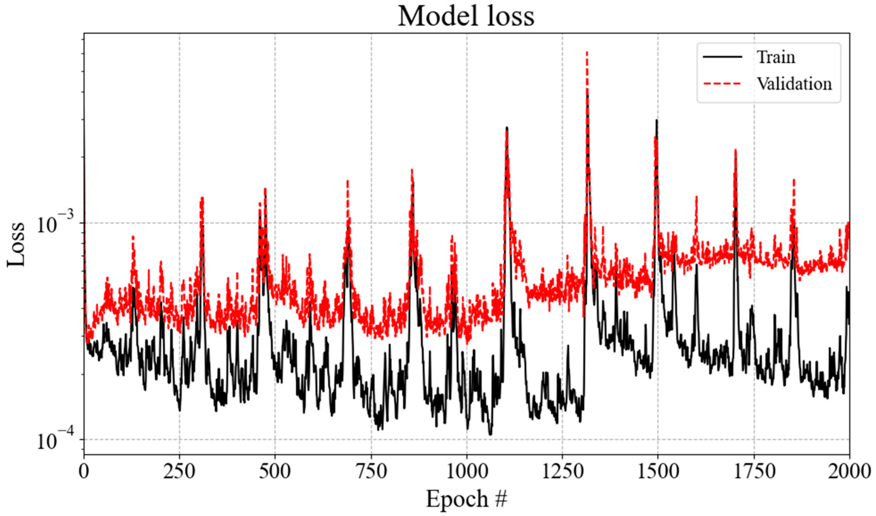
The results of the grid search cross-validation for hyperparameter optimization of the DNN model using a total of 690 source data (1000 TEU) are presented in Figure 9. The mean squared error (MSE) was used to assess the prediction accuracy for each hyperparameter. In this study, three hyperparameters were optimized, and the optimal values for each parameter are as follows; (1) batch size: (4, 8, 16, 32, 64, 128), (2) epochs: (100, 500, 1000, 2000, 3000) and (3) learning rate: (0.001, 0.005, 0.01, 0.05, 0.1). The final hyperparameters determined for the base DNN model were chosen based on the consideration of a small mean squared error value while considering the training speed. The training hyperparameters for the base DNN model were set as follows: batch size = 64, epochs = 2000, and learning rate = 0.01. Using this combination of selected hyperparameters, the model was trained for a total of 18,000 iterations on the 1000 TEU containership dataset. The prediction accuracy of the base DNN training model is quantified by an MSE of approximately 0.0008, as shown in Figure 10. The peak of the loss typically occurs during mini-batch training with split data.

The prediction accuracy for the test dataset not used during training was evaluated to validate the learning level of the base DNN model.

Table 6. MSE, MAPE, and $R^2$ values for the base DNN model.

MSE	MAPE (%)	${\mathit{R}}^2$
0.00081	7.16	0.98

presents the evaluation metrics for the test dataset of the source data, which is the 1000 TEU containership. MSE and MAPE indicate higher prediction accuracy as their values become smaller, and an $R^2$ value closer to 1 signifies that the test dataset not used in training is being well predicted. The DNN model can accurately predict viscous resistance and wake distribution in the propeller plane, as evidenced by the high level of accuracy. Figure 11 displays the predicted viscous resistance results for the two above-mentioned test cases. The average error of the viscous resistance coefficient of model $C_{VM}$ is significantly small, being $0.00009\times {10}^{-0}$, which is less than 0.005% of the target value. 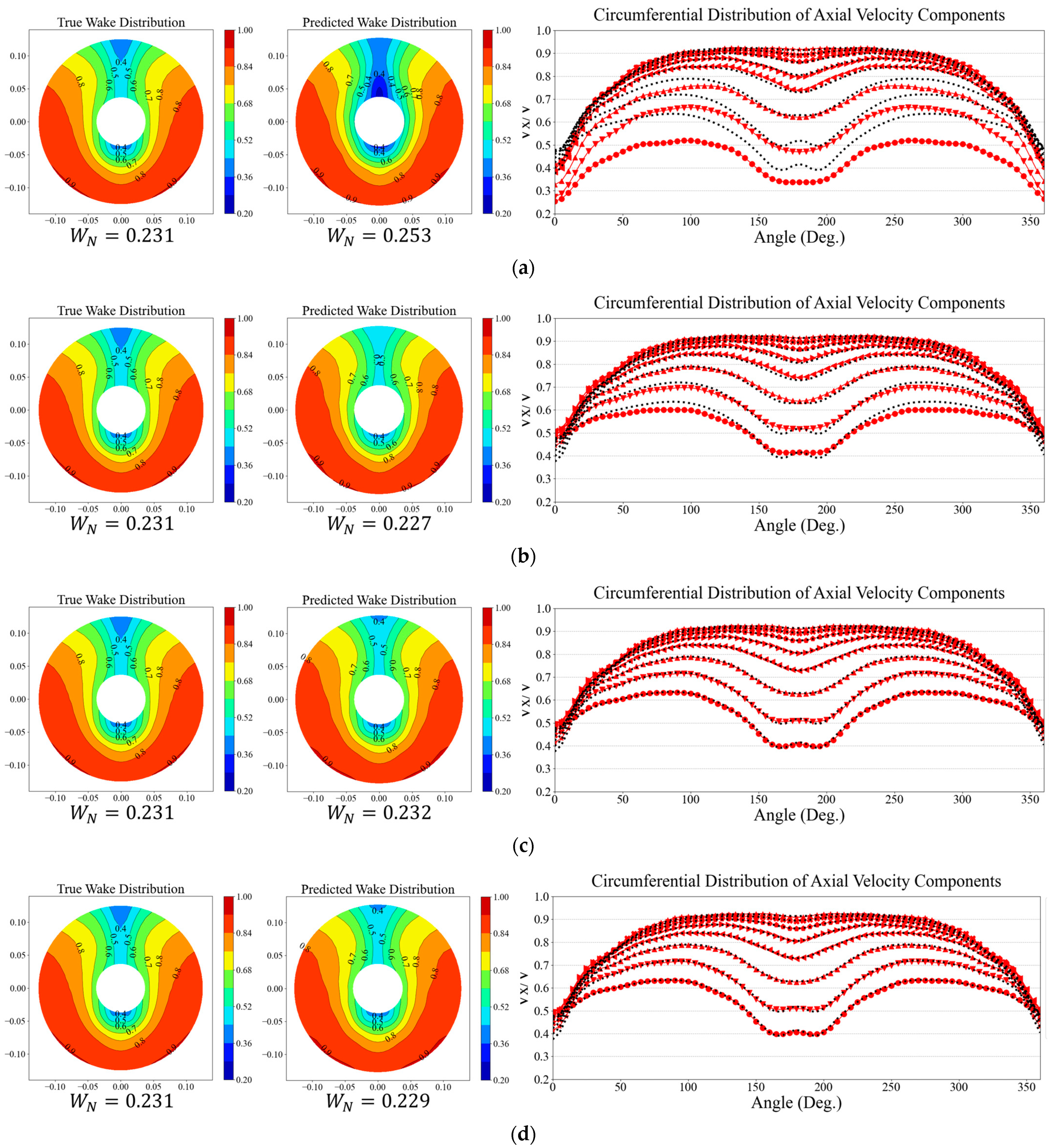Figure 12 compares the true data obtained from CFD analysis with the results predicted by the DNN. The true wake distribution is given on the left, and the predicted data are shown on the right. The true data for the circumferential distribution of the axial velocity component are depicted as black dashed lines, while the predicted data are represented by red symbols and solid lines. As observed in Figure 12, the true and predicted data closely match with high accuracy. In addition, the predicted nominal wake fractions $w_M$ are different from the true values only by less than 0.001, which corresponds to 0.39% error. Here, the nominal wake fraction is computed as follows:

Circumferential mean velocity of each component, $V_{mean}$ is the averaged value of the velocity at the corresponding radius and can be calculated as:

$$V_{mean}=\frac{1}{2\pi }{\int }_0^{2\pi }{V}_i\left(\phi \right)d\phi$$

(17)

Total nominal mean velocity is obtained from the value of circumferential axial mean velocity between radius of propeller hub, $R_{hub}$ and radius of the propeller, $R$ at the propeller plane and computed as follows:

$$V_{Tot,mean}=\frac{2\pi {\int }_{R_{hub}}^R{V}_{mean}·r dr}{\pi ·\left(R^2-R_{hub}^2\right)}$$

(18)

This further leads to the calculation of the nominal wake fraction $w_M$ as follows:

$$w_N=1-\frac{V_A}{V}=1-V_{Tot,mean}$$

(19)

The DNN model is capable of accurately predicting not only wake distribution but also viscosity resistance. The neural network that serves as the basis for transfer learning on a small amount of data requires sufficient prediction accuracy. Given the results above, it can be concluded that the base DNN model can effectively capture the design variables of the FCF and establish a strong association with both the viscous resistance coefficient and wake distribution, demonstrating high accuracy in its predictions.

4.3. Prediction Results Using Target Dataset (DNN-TL Model)

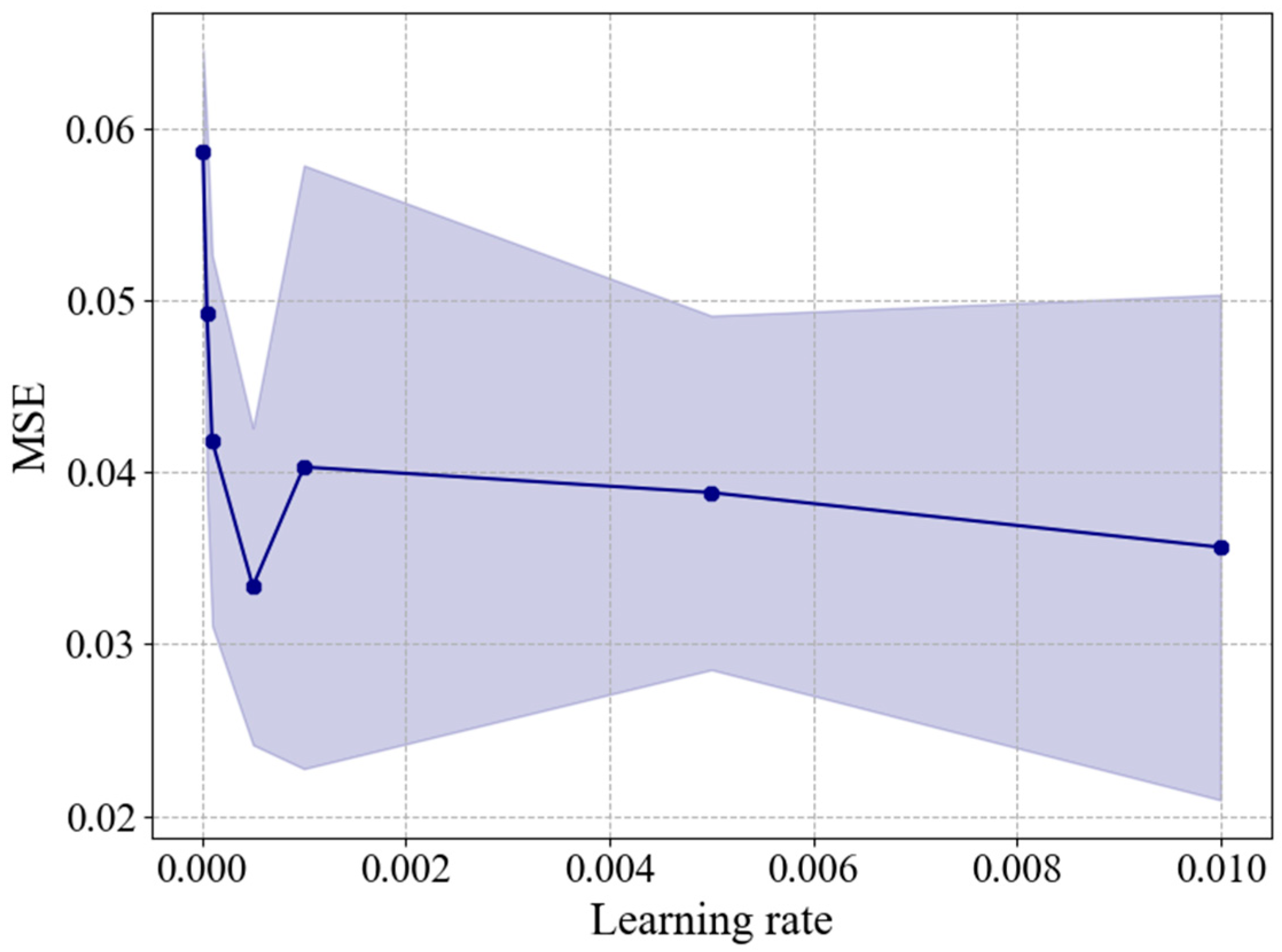
The DNN-TL model is reconstructed and retrained based on the weights of the previously trained DNN model, using only the target dataset. Since the size of the target dataset is considerably smaller (150 datasets) compared to the source dataset, a smaller learning rate is necessary to ensure training accuracy. Therefore, it is necessary to find the optimal learning rate value for the training dataset of the DNN-TL model. The optimization was performed with learning rates (0.00001, 0.00005, 0.0001, 0.0005, 0.001, 0.005, 0.01), and the comparison of MSE values for each value is shown in Figure 13. In this study, the optimal learning rate value for predicting the viscous resistance and wake distribution of the target dataset (2500 TEU and 3600 TEU) is determined to be 0.0005. Based on this, the parameters of the DNN-TL model were constructed. To verify the prediction of viscous resistance and wake distribution based on transfer learning, different configurations were tested: DNN-TL models with 1, 4, and 5 fixed layers, as well as a DNN-TL model without any fixed layers (

Table 7. Fine-tuning for DNN-TL.

	1st Hidden Layer	2nd Hidden Layer	3rd Hidden Layer	4th Hidden Layer	5th Hidden Layer
All fixed layer	Fixed	Fixed	Fixed	Fixed	Fixed
Fixed 4 layer	Fixed	Fixed	Fixed	Fixed	Train
Fixed 1 layer	Fixed	Train	Train	Train	Train
No fixed layer	Train	Train	Train	Train	Train

). Fine-tuning was performed on each of these configurations, and their performances were compared. In the DNN-TL model, the weights of neurons are initialized based on the previously trained base model, and the model is retrained and reconstructed using the training dataset from the target dataset.

The prediction accuracy based on the fine-tuning of hidden layer weights was evaluated to verify the level of learning. Figure 14 compares the predicted viscous resistance coefficients of the model ship for each fine-tuning condition. The black-filled bar chart represents the true values obtained from CFD analysis, while the red dashed-filled bars represent the predicted results from each fine-tuning condition. The viscosity resistance performance was compared using one test dataset for each of the 2500 TEU and 3600 TEU containerships. Figure 15 and Figure 16 illustrate the comparison of predicted results for harmonic wake distribution and circumferential distribution of axial velocity components for both 2500 TEU and 3600 TEU. The left figure shows the harmonic wake distribution obtained from CFD analysis, and the middle part displays the predicted wake distribution from each fine-tuning condition. In the case where the weights of all five hidden layers are fixed (the all fixed layer case), there is an error of 18% specifically in the viscosity resistance coefficient ($C_{VM}$) for the 3600 TEU containership. The accuracy of predicting the axial velocity distribution in the propeller plane is also quite low, and it can be observed that it is trying to follow the wake distribution characteristics of the 1000 TEU used in the base DNN model. In the case of “Fixed 4 layer”, where only the weights of the last layer among the layers were trained, $C_{VM}$ for 2500 TEU and 3600 TEU show errors of 0.38% and −3.6%, respectively. This indicates an improvement in prediction accuracy compared to the “All fixed layer” case. In Figure 15b and Figure 16b, compared to the “All fixed layer”, there is an attempt to capture the characteristics of each hull form. This indicates that the weights of the last hidden layer among the hidden layers play a role in conveying a certain level of knowledge about the target datasets (2500 TEU and 3600 TEU). The prediction results for the fixed 1 layer, where only the weights of the first hidden layer are not retrained, and the no fixed layer, where all layers are retrained, show a quite similar trend. The $C_{VM}$ prediction results for both 2500 TEU and 3600 TEU exhibit errors within 0.5%. When observing the wake distribution and axial velocity components figures, it is evident that the characteristics of each linear component are sufficiently captured. Furthermore, the errors in the nominal wake fraction $w_M$ between the TL predictions and the true values are 0.0 for the 2500 TEU (Figure 15c) and 0.001 (Figure 16c), which amounts to 0% and 0.43%, respectively. This exemplifies the accuracy of the present TL prediction in wake field prediction.

Table 8. MSE, MAPE, and $R^2$ values for each fine-tuning condition.

	MSE	MAPE (%)	${\mathit{R}}^2$
All fixed layer	0.3083	182.4	−4.163
Fixed 4 layer	0.0307	24.88	0.499
Fixed 1 layer	0.0086	13.89	0.854
No fixed layer	0.0185	18.40	0.703

presents the prediction accuracy metrics for the test dataset that was not used in the training process under each fine-tuning condition. MSE and MAPE are metrics where lower values indicate higher accuracy in predictions. $R^2$, on the other hand, is a measure of how well the model explains the variance in the data. A higher $R^2$ value, closer to 1, indicates a better predictive performance. Generally, when $R^2>0.67$, it is considered to have a reasonably good predictive accuracy, while $0.33<R^2<0.67$ indicates moderate predictive performance, and $0.16<R^2<0.32$ suggests poor predictive performance [21]. The $R^2$ score for the “All fixed layer” case is −4.163, indicating no prediction capability on the test dataset. Conversely, when the first hidden layer is fixed, it exhibits the highest scores across all accuracy metrics. It is considered that the weights of the first layer in the previously trained base DNN model were tailored to capture the characteristics of the viscous resistance coefficient on the containership and the axial velocity on the propeller plane. The remaining hidden layers seem to have been designed to understand the fluid characteristics by hull form. To assess the level of prediction accuracy in this study, the performance was compared to accuracy metrics from other literature that used transfer learning for predictions. Solis and Calvo-Valverde [22] applied DNN and TL to time series prediction, and their optimal prediction model achieved an MAPE value of approximately 9%. Zhou et al. [23] predicted the dynamic behavior of a gas turbine engine using transfer learning, and in their optimal prediction model, they achieved MSE and $R^2$ values of 0.00466 and 0.881, respectively. The MSE, MAPE, and $R^2$ values in this paper all fall within a similar range, indicating that the prediction model applied with transfer learning is at a satisfactory level of accuracy.

Figure 17 compares the predicted radial profiles of axial velocity components from the four tuning cases with their true values. The green circles represent the predictions from the “All fixed layer” condition, the black squares are from the case where the first four layers were fixed (fixed 4 layer), the blue triangles represent the condition where only the first layer was fixed (fixed 1 layer), and the red “X” symbols depict the predictions from the “No fixed layer” condition. In the case of “All fixed layer”, significant discrepancies are observed between the predicted values and the true values across all radii. On the other hand, for the “Fixed 1 layer” and “No fixed layer” cases, it can be observed that the predicted values closely follow the trends of the true values.

5. Conclusions

This paper proposes a novel methodology for predicting the resistance performance and wake distribution of flow control fins (FCFs) on containerships of various sizes using deep neural networks (DNN) through transfer learning. The main contribution of this paper lies in introducing DNN to predict the outcomes in a shorter time compared to traditional computational fluid dynamics (CFD) simulations, which are used to assess the performance based on the locations of FCFs on containerships of different sizes. Another novel aspect is the utilization of transfer learning (TL) to enhance the efficiency of training using a limited amount of data. Firstly, a base DNN model is constructed based on a relatively large source dataset of 690 cases (1000 TEU). Then, transfer learning is applied to predict the performance of smaller target datasets (2500 TEU and 3600 TEU) using the base DNN model as a foundation. Furthermore, fine-tuning between layers in the transfer learning process is employed to identify the conditions that yield the highest learning accuracy.

As a result, the first layer of the base DNN model was fixed, and the rest of the layers were retrained and reconfigured conditions showed higher scores in accuracy metrics. When evaluated using the test dataset that was not involved in the transfer learning training, the MSE, MAPE, and $R^2$ were found to be 0.0086, 13.89%, and 0.854, respectively, indicating the highest accuracy. Additionally, in terms of the viscous resistance coefficient ($C_{VM}$), the accuracy was within 0.5%. This study demonstrates the procedure in which machine learning techniques, particularly transfer learning, can contribute to the advancement of computational design technology. The machine learning methodologies developed in this study can be utilized to design and optimize the FCFs for similar vessels with different sizes in the class of feeder containerships under 4000 TEUs.

The current application of transfer learning-based predictive capabilities is not limited to specific case studies. By adopting the optimization techniques, it could be extended to the optimal design of FCFs’ positions for various types of containerships, which will be the topic of future study. However, predicting the performance of FCF applied to a full-scale vessel requires conducting high Reynolds number simulations, and currently, performing simulations at the full-scale is a challenging issue in fluid performance research. Predicting the viscous resistance and axial velocity performance at the propeller plane for a full-scale vessel with FCF application remains a significant challenge.

References

1. Samsung Heavy Industry. Flow Control Appendages for Improvement of Pressure Resistance and Hull Vibration. Korean Patent 1007189340000 B1, 10 May 2007.
2. Lee, H.D.; Hong, C.B.; Kim, H.T.; Choi, S.H.; Han, J.M.; Kim, B.; Lee, J.H. Development and application of energy saving devices to improve resistance and propulsion performance. In Proceedings of the the Twenty-Fifth International Ocean and Polar Engineering Conference, Kailua-Kona, HI, USA, 21–26 June 2015. [Google Scholar]
3. Kim, D.J.; Oh, W.J.; Park, J.W.; Jeong, S.M. A Study on Flow Characteristics due to Dimension Variations of the Vertical Plate for Controlling the Ship Stern Flow. J. Korean Soc. Mar. Environ. Saf. 2016, 22, 576–582. [Google Scholar] [CrossRef]
4. Lee, J.; Kim, I.; Park, D.W. A Study on the Resistance Performance and Flow Characteristic of Ship with a Fin Attached on Stern Hull. J. Korean Soc. Mar. Environ. Saf. 2021, 27, 1106–1115. [Google Scholar] [CrossRef]
5. Park, Y.; Hwangbo, S.M.; Yu, J.-W.; Cho, Y.; Lee, J.H.; Lee, I. Development of a small-sized tanker with reduced greenhouse gas emission under in-service condition based on CFD simulation. Ocean Eng. 2022, 286, 115588. [Google Scholar] [CrossRef]
6. Hwangbo, S.; Shin, H. Statistical prediction of wake fields on propeller plane by neural network using back-propagation. J. Ship Ocean Technol. 2000, 4, 1–12. [Google Scholar]
7. Kim, S.-Y.; Moon, B. Wake distribution prediction on the propeller plane in ship design using artificial intelligence. Ships Offshore Struct. 2006, 1, 89–98. [Google Scholar] [CrossRef]
8. Wie, D.-E.; Kim, D.-J. The Design Optimization of a Flow Control Fin Using CFD. J. Soc. Nav. Archit. Korea 2012, 49, 174–181. [Google Scholar] [CrossRef]
9. Liu, X.; Wan, D.; Lei, L. Multi-fidelity model and reduced-order method for comprehensive hydrodynamic performance optimization and prediction of JBC ship. Ocean Eng. 2023, 267, 113321. [Google Scholar] [CrossRef]
10. Feng, Y.; Chen, Z.; Dai, Y.; Wang, F.; Cai, J.; Shen, Z. Multidisciplinary optimization of an offshore aquaculture vessel hull form based on the support vector regression surrogate model. Ocean Eng. 2018, 166, 145–158. [Google Scholar] [CrossRef]
11. Su, Y.; Lin, J.; Zhao, D.; Guo, C.; Wang, C.; Guo, H. Real-time prediction of large-scale ship model vertical acceleration based on recurrent neural network. J. Mar. Sci. Eng. 2022, 8, 777. [Google Scholar] [CrossRef]
12. Mittendorf, M.; Nielsen, U.D.; Bingham, H.B. Data-driven prediction of added-wave resistance on ships in oblique waves—A comparison between tree-based ensemble methods and artificial neural networks. Appl. Ocean Res. 2022, 118, 102964. [Google Scholar] [CrossRef]
13. Lin, J.; Han, Y.; Guo, C.; Su, Y.; Zhong, R. Intelligent ship anti-rolling control system based on a deep deterministic policy gradient algorithm and the Magnus effect. Phys. Fluids 2022, 34, 057102. [Google Scholar] [CrossRef]
14. Lee, M.-K.; Lee, I. Optimal Design of Flow Control Fins for a Small Container Ship Based on Machine Learning. J. Mar. Sci. Eng. 2023, 11, 1149. [Google Scholar] [CrossRef]
15. Kim, J.H.; Choi, J.E.; Choi, B.J.; Chung, S.H.; Seo, H.W. Development of energy-saving devices for a full slow-speed ship through improving propulsion performance. Int. J. Nav. Archit. Ocean Eng. 2015, 7, 390–398. [Google Scholar] [CrossRef]
16. ITTC. Uncertainty Analysis in CFD, Verification and Validation Methodology and Procedures, Recommended Procedures and Guidelines. Int. Towing Tank Conf. 2017, 7.5-03-01-01, 4–8. [Google Scholar]
17. Qiao, J.; Liu, X.; Chen, Z. Prediction of the remaining useful life of lithium-ion batteries based on empirical mode decomposition and deep neural networks. IEEE Access 2020, 8, 42760–42767. [Google Scholar] [CrossRef]
18. Babaeiyazdi, I.; Rezaei-Zare, A.; Shokrzadeh, S. Transfer Learning With Deep Neural Network for Capacity Prediction of Li-Ion Batteries Using EIS Measurement. IEEE Trans. Transp. Electrif. 2022, 9, 886–895. [Google Scholar] [CrossRef]
19. Shen, S.; Sadoughi, M.; Li, M.; Wang, Z.; Hu, C. Deep convolutional neural networks with ensemble learning and transfer learning for capacity estimation of lithium-ion batteries. Appl. Energy 2020, 260, 114296. [Google Scholar] [CrossRef]
20. Park, K.M. Machine classification in ship engine rooms using transfer learning. J. Korean Soc. Mar. Environ. Saf. 2021, 27, 363–368. [Google Scholar] [CrossRef]
21. Chin, W.W.; Marcolin, B.L.; Newsted, P.R. A partial least squares latent variable modeling approach for measuring interaction effects: Results from a Monte Carlo simulation study and an electronic-mail emotion/adoption study. Inf. Syst. Res. 2003, 14, 189–217. [Google Scholar] [CrossRef]
22. Solís, M.; Calvo-Valverde, L.A. Performance of Deep Learning models with transfer learning for multiple-step-ahead forecasts in monthly time series. arXiv 2022, arXiv:2203.11196. [Google Scholar] [CrossRef]
23. Zhou, D.; Hao, J.; Huang, D.; Jia, X.; Zhang, H. Dynamic simulation of gas turbines via feature similarity-based transfer learning. Front. Energy 2020, 14, 817–835. [Google Scholar] [CrossRef]
Figure 1. Three-dimensional volumetric views of target hulls and propellers: (a) 1000 TEU; (b) 2500 TEU; (c) 3600 TEU.
Jmse 11 01898 g001aJmse 11 01898 g001b
Figure 2. Geometry of FCF.
Jmse 11 01898 g002
Figure 3. Features distribution for each containership: (a) distribution of viscous resistance coefficient; (b) standard deviation of axial velocity distribution.
Jmse 11 01898 g003
Figure 4. Computational domain for double body simulation.
Jmse 11 01898 g004
Figure 5. The general architecture of the DNN model.
Jmse 11 01898 g005
Figure 6. Preprocessing of output data for the neural network: (a) bisecting the propeller plane; (b) harmonic analysis.
Jmse 11 01898 g006
Figure 7. Overview of the transfer learning.
Jmse 11 01898 g007
Figure 8. Workflow of transfer learning.
Jmse 11 01898 g008
Figure 9. Grid search results for DNN model using source dataset.
Jmse 11 01898 g009
Figure 10. Loss for the base DNN models.
Jmse 11 01898 g010
Figure 11. Evaluation of prediction accuracy by the viscous resistance coefficient for the base DNN model.
Jmse 11 01898 g011
Figure 12. Evaluation of prediction accuracy by harmonic wake distribution and axial wake distribution for the base DNN model: (a) test data no.1; (b) test data no.2.
Jmse 11 01898 g012
Figure 13. Optimization of the learning rate for DNN-TL model using target dataset.
Jmse 11 01898 g013
Figure 14. Evaluation of prediction accuracy by the viscous resistance coefficient for the target dataset (2500 TEU and 3600 TEU) between each fine-tuning condition.
Jmse 11 01898 g014
Figure 15. Evaluation of prediction accuracy by harmonic wake distribution and axial wake distribution for 2500 TEU between each fine-tuning condition: (a) all fixed; (b) fixed 4 layer; (c) fixed 1 layer; (d) no fixed layer.
Jmse 11 01898 g015
Figure 16. Evaluation of prediction accuracy by harmonic wake distribution and axial wake distribution for 3600 TEU between each fine-tuning condition: (a) all fixed; (b) fixed 4 layer; (c) fixed 1 layer; (d) no fixed layer.
Jmse 11 01898 g016
Figure 17. Predictions for the circumferential distribution of axial velocity components for each radius: (a) R = 0.30; (b) R = 0.40; (c) R = 0.50; (d) R = 0.60; (e) R = 0.70; (f) R = 0.80; (g) R = 0.90; (h) R = 1.00.
Jmse 11 01898 g017aJmse 11 01898 g017b