Numerical Generation of Solitary Wave and Its Propagation Characteristics in a Step-Type Flume

Abstract

This work concerns the numerical generation of stable solitary waves by using a piston-type wave maker and the propagation characteristics of a solitary wave in a step-type flume. The numerical generation of solitary waves was performed by solving N-S (Navier–Stokes) equations on the open source CFD (computational fluid dynamics) platform OpenFOAM. To this end, a new module of dynamic boundary conditions was programmed and can be applied to prescribe the horizontal linear motion of a paddle. Two kinds of paddle motions, based on both the first-order and ninth-order solutions of solitary waves, were first determined. The time history of paddle motion was restored in a file, which was then used as an input for the virtual wave maker. The solitary wave in water with a constant depth was generated by both numerical simulation and experiment in the wave flume installed with a piston wave maker. The results show that the amplitudes of trailing waves based on the first-order solution are larger than those based on the ninth-order solution and that wave height based on the first-order solution decays more quickly. The numerical wave profiles are in good agreement with the experimental ones. The propagation characteristics of a solitary wave in a step-type flume was numerically investigated as well. It was found that a part of the solitary wave is reflected when the solitary wave passes the step due to blockage effects, and the forward main wave collapses quickly when it enters shallow water. This work presents a very successful numerical study of stable solitary wave generation and reveals the phenomena when a solitary wave propagates in a step-type flume.

1. Introduction

A tsunami wave could lead to significant adverse damage to our coastal community. It normally propagates from a deep-sea area to a nearshore area, consequently leading to a strong destruction of coastal and offshore structures. Thus, its propagation characteristics have always be a focused topic. After traveling a long distance, a tsunami wave evolves into N-waves or successive solitary waves [1,2]. As a result, we usually study solitary waves instead of tsunami waves. One of main efforts regarding this topic is how to generate a solitary wave and to reveal its propagation characteristics.

Extensive studies on the generation of solitary waves, as well as their propagation and evolution, have been reported in history. [3], who derived the Boussinesq equations based on the Euler equations, contributed a lot in theory. The Boussinesq equations are a set of first-order equations which can be employed to describe a solitary wave. Soon after, the other first-order solution, by Rayleigh [4], was also derived. Since then, several approximate higher-order theories have been promoted to describe a solitary wave more accurately, e.g., the third-order solution by Grimshaw [5] and the ninth-order solution by Fenton [6]. These theories offer a great foundation for the generation of a solitary wave in a laboratory. Goring [7] derived the relationship between the horizontal movement of a piston-type wave maker and the solitary wave profile on the basis of Boussinesq’s solitary wave solution. Based on this method, Katell and Eric [8] developed a new experimental procedure, which was derived from Rayleigh’s [4] solitary wave solution, to generate solitary waves in a flume by using a piston-type wave maker. Their new procedure resulted in less loss of amplitude in the initial stage of the propagation of the solitary waves compared with that by Goring’s [7] procedure. Malek-Mohammadi and Testik [9] recommended a new methodology for the laboratory generation of solitary waves by using piston-type wave makers. The new methodology considered the evolving nature of the wave differently than Goring’s [7] method in which the wave form was assumed to be permanent during the generation process. The new methodology was demonstrated to have the capability of generating more accurate solitary waves with less attenuation.

With the development of the computer, numerical simulation has become an important means for the study of solitary waves. Wu et al. [10] numerically studied the generation and propagation of Boussinesq’s [3], Rayleigh’s [4], Grimshaw’s [5], and Fenton’s [6] solitary waves based on Goring’s method. A mesh-free potential flow model was used. They concluded that the solitary wave based on Fenton’s solution displayed the best performance in obtaining a purer wave shape. Later on, Wu et al. [11] validated the numerical method used in the work of Wu et al. [10] by means of physical experiments, and they confirmed that Fenton’s solution gave the most stable solitary waves. Moreover, the work by Wu et al., [11] also found that the imperfect fitness of the wave paddle to the flume could affect the stability of the solitary wave by a great amount.

Farhadi et al., [12] studied the accurate generation of solitary waves by using an incompressible smoothed particle hydrodynamics (ISPH) method. The influences of the different solitary wave solutions discussed in the works by Katell and Eric [8] and Wu et al. [10] on the resulting wave profile were compared. It was concluded that the ninth-order solution for solitary waves provided more stable waves.

Wu and Hsiao [13] investigated the propagation of solitary waves in water with a constant depth by the numerical models based on various solitary wave theories. The Dirichlet boundary condition and an internal mass source were utilized. One of their conclusions was that the approach of internal wave makers required a higher-order solitary wave solution to generate accurate and stable solitary waves.

Francis et al. [14] used two solitary wave generation methodologies, i.e., Goring’s [7] method and the method by Malek-Mohammadi and Testik [9], to generate solitary waves experimentally and numerically. The four solitary wave solutions, as discussed by Wu et al., [10], were also adopted in their study. The results indicated that Rayleigh’s solitary wave solution displayed more accurate profiles in both experiments and numerical simulations. With respect to wave generation methodology, the latter method gave the best results in experiments, whereas the former method described the targeted wave better in numerical simulations.

Huang and Dong [15] studied the interaction between a solitary wave and a submerged dike by solving the N-S (Navier–Stokes) equations. The accuracy of the numerical scheme was verified by comparing the analytical solutions for the case of a flatbed wave tank. The study suggested that the primary vortex generated at the lee side of the dike and the secondary vortex at the right toe of the dike might scour the bottom and cause a severe problem for the dike. In practice, the propagation and evolution characteristics of solitary waves in such real water areas are more interesting, e.g., the characteristics of such waves in water of variable depth or the interactions between solitary waves and offshore/nearshore structures. In this regard, more and more publications have reported relevant works in recent years. For example, Xuan et al., [16] conducted experiments to investigate the run-up of two solitary waves on plane beaches. Ghafari et al., [17] presented an experimental and numerical investigation of solitary wave interactions with two submerged rectangular obstacles. Goral et al. [18] experimentally studied the dynamic responds of solid spheres in solitary waves. Wu et al. [19] performed a study on the problem of the run-up of breaking solitary waves on uniform slopes.

The present work concerns the generation of stable solitary waves by using a piston-type wave maker and the propagation characteristics of a solitary wave in a step-type flume. For the purpose of generating solitary waves, the open source CFD (computational fluid dynamics) tool OpenFOAM was employed to solve the N-S equations. The VOF (volume of fluid) method was used to model the water–air flow. The mesh deformation approach was used to simulate the linear motion of the paddle. Great efforts contributed to the programming of a new dynamic wall boundary condition in OpenFOAM. Specifically, a detailed study was performed for the dependency analyses of grid density and time step for the resulting wave profile, which was not performed in the most of previous works. In order to check the effectives of the present numerical method, experiments in the wave flume at the Wuhan University of Technology were conducted. The qualities of the generated waves based on the first-order and ninth-order solutions of solitary wave were compared. The propagation process of a solitary wave in a step-type flume is was analyzed and discussed as well. This work presents a very successful numerical method for the generation of solitary waves and reveals the phenomena when a solitary wave enters from deep water into shallow water.

2. Generation of a Solitary Wave by Piston-Type Wave Maker

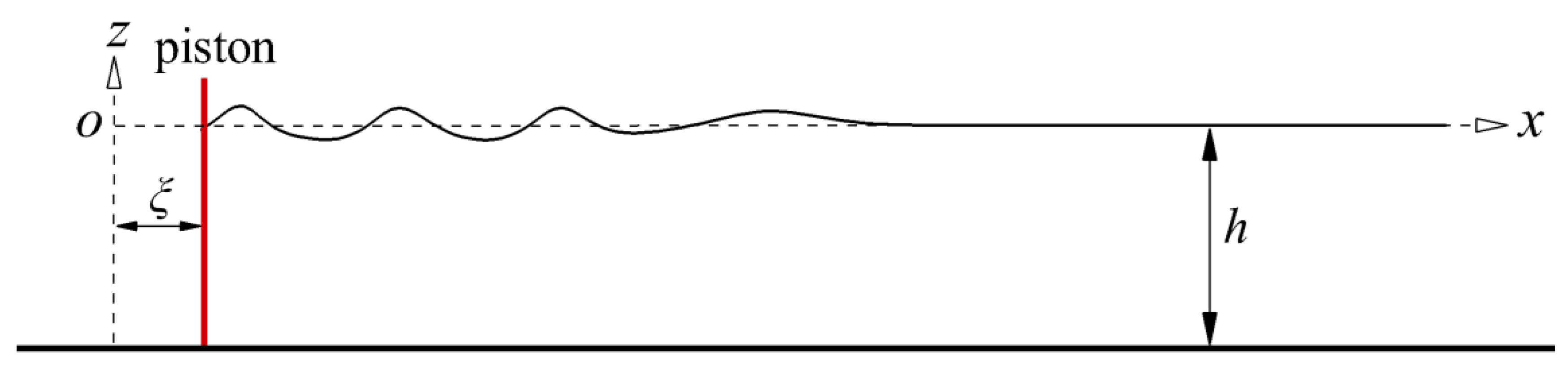
The schematic diagram of wave generation in a two-dimensional flume by using a piston-type wave maker is illustrated in Figure 1. A Cartesian coordinate is defined to describe the motion of the paddle and the resulting wave profile. The origin locates on the water surface in the still water with a depth of $h$, the x-axis towards right side, and the z-axis vertically upwards. The paddle can perform a linear motion along the horizontal axis. At beginning, i.e., zero time, it is assumed that the paddle locates on the z-axis. According to the theory of wave generation, if the paddle moves in a certain manner, e.g., the time history of the paddle displacement $\xi \left(t\right)$ is prescribed, a targeted wave will be produced in the flume. When generating linear waves, $\xi$ is a sine or cosine function of time.

For the generation of a solitary wave, according to the work by Goring [7], the relationship between the linear motion of the paddle and the resulting profile of solitary wave can be formulated by

$$\frac{d\xi }{dt}=\overline{U}=\frac{c\eta {|}_{x=\xi }}{h+\eta {|}_{x=\xi }}$$

(1)

where $\overline{U}$ is the depth-averaged horizontal water particle velocity near the paddle or the paddle linear velocity, $\eta$ is the wave evaluation, c is the wave phase speed, and t is the time. The water surface evaluation is expressed by

$$\eta =H{s}^2$$

(2)

where H is the wave height. The expressions of s, k, and c are as follows.

$$s=\mathrm{sech}\left[k\left(\xi -ct\right)\right]$$

(3)

$$k=\sqrt{\frac{3H}{4h^3}}$$

(4)

$$c=\sqrt{g\left(h+H\right)}$$

(5)

where k is the effective wave number.

Integrating Equation (1), the exact solution of first-order paddle displacement can be obtained.

$$\xi (t)=\frac{H}{kh}\tan \mathrm{h}[k(ct-\xi \left)\right]$$

(6)

The asymptotic solution of motion stroke $S$ is then as follows.

$$S=\xi (+\infty )-\xi (-\infty )=\sqrt{\frac{16H}{3h}}h$$

(7)

Note that the solitary wave solution used by Goring [7] is of the first order. Based on the ninth-order solution of the solitary wave by Fenton [6], the water surface evaluation is expressed by

$$\eta =h{{\displaystyle \sum _{i=1}^9{\eta }_i\left(\frac{H}{h}\right)}}^i,$$

(8)

The corresponding ninth-order $k$ and $c$ are then

$$k=\sqrt{\frac{3H}{4h^3}}{{\displaystyle \sum _{i=0}^8{k}_i\left(\frac{H}{h}\right)}}^i,$$

(9)

$$c=\sqrt{gh\left(1+{\displaystyle \sum _{i=1}^9{c}_i{\left(\frac{H}{h}\right)}^i}\right)}$$

(10)

where the formulas or values of ${\eta }_i$, $k_i$, and $c_i$ are listed in

Table 1. The formulas or coefficients for the ninth-order solitary wave solution.

i	${\mathit{\eta }}_{\mathit{i}}$	${\mathit{k}}_{\mathit{i}}$	${\mathit{c}}_{\mathit{i}}$
0	---	1.000000	---
1	$s^2$	1.000000	1.000000
2	$-0.75s^2+0.75s^4$	−0.625000	−0.050000
3	$0.625s^2-1.8875s^4+1.625s^6$	0.554688	−0.042857
4	$-1.36817s^2+3.88033s^4-4.68304s^6+2.17088s^8$	−0.561535	−0.034286
5	$1.86057s^2-7.45136s^4+12.7637s^6-11.4199s^8+4.24687s^{10}$	0.567095	−0.031520
6	$-2.57413s^2+13.2856s^4-31.1191s^6+40.1068s^8$ $-28.4272s^{10}+8.728s^{12}$	−0.602969	−0.029278
7	$3.4572s^2-22.782s^4+68.258s^6-116.974s^8+120.49s^{10}$ $-71.057s^{12}+18.608s^{14}$	0.624914	−0.026845
8	$-4.6849s^2+37.67s^4-139.28s^6+301.442s^8-411.416s^{10}$ $+355.069s^{12}-180.212s^{14}+41.412s^{16}$	−0.670850	−0.030263
9	$6.191s^2-60.57s^4+269.84s^6-712.125s^8+1217.98s^{10}$ $-1384.37s^{12}1023.07s^{14}-450.29s^{16}+90.279s^{18}$	0.700371	−0.021935

.

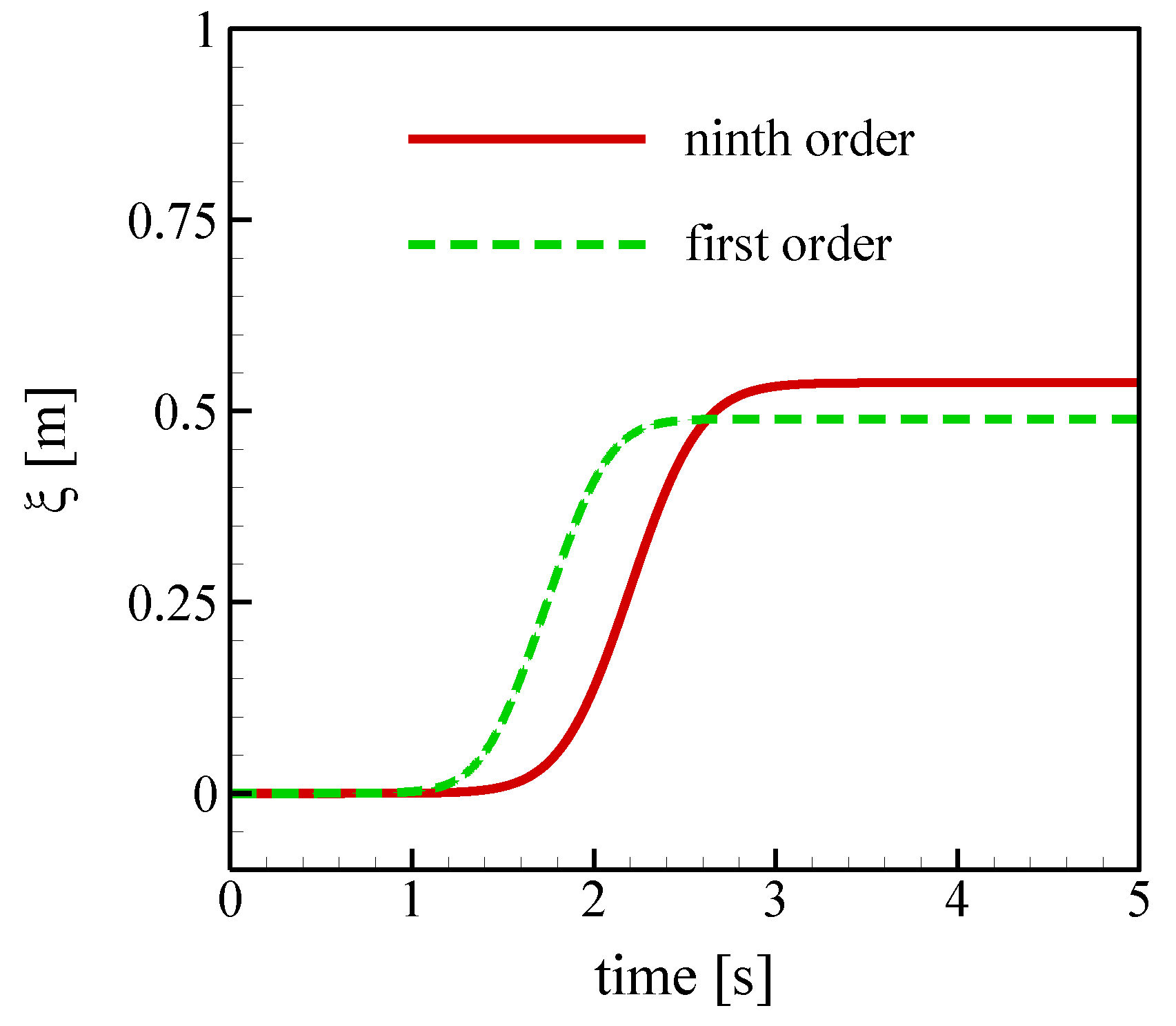
If the water depth and wave height are known, substituting Equation (2) or Equation (8) into Equation (1) and solving Equation (1), the time history of the paddle displacement can be determined. Here a numerical method is applied to solve Equation (1). The explicit Euler scheme is used to discretize the time term in Equation (1). Figure 2 presents the resulting time histories of the paddle displacement based on both the first-order and ninth-order solutions of solitary waves for the case of constant water depth 0.3 m and wave height 0.15 m, i.e., the relative wave height is 0.5. The maximum paddle displacement based on the ninth-order solution is around 0.5371 m. However, it is 0.4899 m for the first-order solution, which is identical with the asymptotic solution of the stroke calculated by Equation (7). For the ninth-order solution, the paddle pushes forward more water.

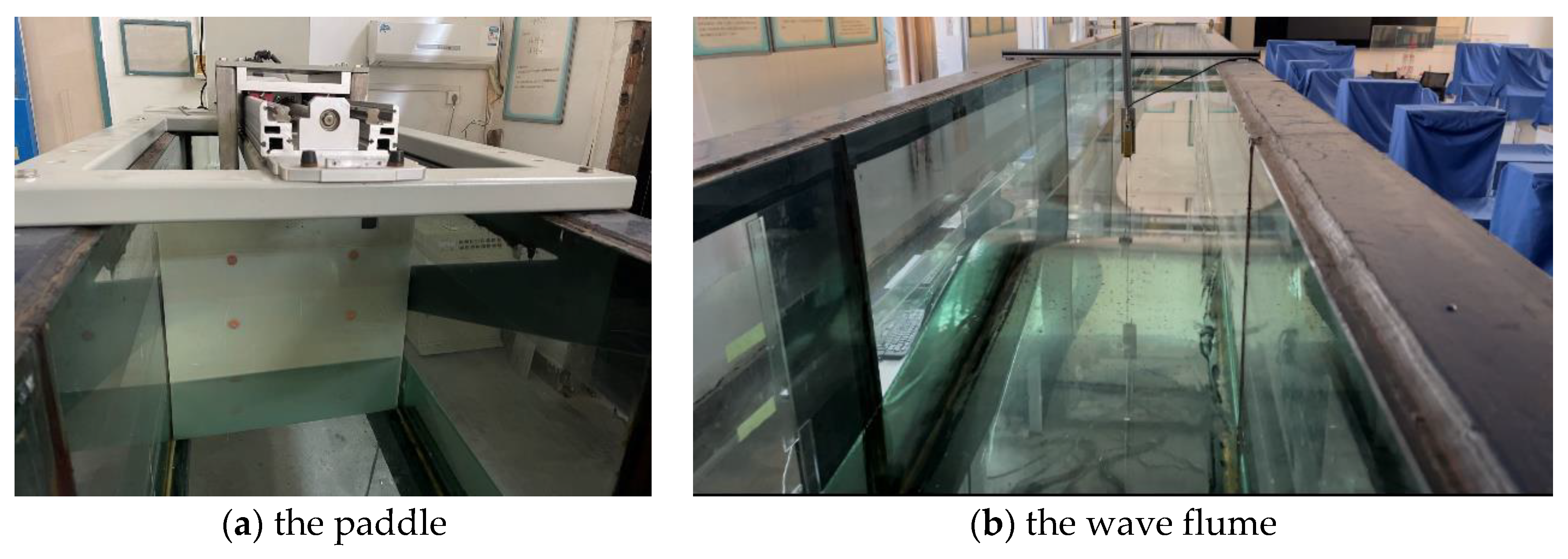
In the present study, solitary waves are numerically generated by solving N-S equations in water with a depth of 0.3 m. The targeted wave height is 0.15 m. In order to validate the numerical results, experiments were carried out at the Wuhan University of Technology. The wave flume is 18 m in length, 0.6 m in width, and 0.8 m in depth. The flume walls are made of glass. Figure 3 shows the wave generation system. Two wave gauges are installed to record water surface evaluation. The probes are located on the center line of the flume. During the experiments, the paddle motion is controlled by a computer. Once the wave height and water depth are pre-set, the control software first solves Equation (1) so as to determine the time history of the paddle displacement, which is as an input for the wave generation system. The paddle, which is driven by a motor, then moves according to the time history of the linear motion.

3. Numerical Method

3.1. Governing Equations

The N-S equations, together with the continuity equation, are solved by a finite volume method to generate solitary waves. The open source CFD tool OpenFOAM was employed for this purpose, as mentioned. Under the assumption of incompressible fluid, the continuity equation and N-S equations, which are expressed in the coordinate system as shown in Figure 1, can be written as

$$\frac{\partial u}{\partial x}+\frac{\partial w}{\partial z}=0,$$

(11)

$$\frac{\partial u}{\partial t}+u\frac{\partial u}{\partial x}+w\frac{\partial u}{\partial z}=-\frac{1}{\rho }\frac{\partial p}{\partial x}+\nu \left(\frac{{\partial }^{2}u}{\partial x^2}+\frac{{\partial }^{2}u}{\partial z^2}\right),$$

(12)

$$\frac{\partial w}{\partial t}+u\frac{\partial w}{\partial x}+w\frac{\partial w}{\partial z}=-g-\frac{1}{\rho }\frac{\partial p}{\partial z}+\nu \left(\frac{{\partial }^{2}w}{\partial x^2}+\frac{{\partial }^{2}w}{\partial z^2}\right).$$

(13)

where u and w are the components of flow velocity, $\nu$ is the viscosity coefficient, p is the dynamic pressure, ρ is the density, and g is the acceleration due to gravity.

The free surface is captured by using the available VOF method. The governing equation of volume fraction F is as follows.

$$\frac{\partial F}{\partial t}+\frac{\partial \left(Fu\right)}{\partial x}+\frac{\partial \left(Fw\right)}{\partial z}=0,$$

(14)

where if F = 1, the cell is full of water; if F = 0, the cell is full of air; and if 0 < F < 1, the cell locates at the interface between water and air. The density and viscosity coefficients of the water–air flow in Equations (12) and (13) are computed by

$$\rho =F{\rho }_w+\left(1-F\right){\rho }_e,$$

(15)

$$\nu =F{\nu }_w+\left(1-F\right){\nu }_e,$$

(16)

where ${\rho }_w$, ${\nu }_w$ are the density and the viscosity coefficients of water, and ${\rho }_e$, ${\nu }_e$ are the density and the viscosity coefficients of air.

OpenFOAM supplies a suite of discretization schemes for the terms of time, convection, and diffusion in N-S equations, respectively, and the solvers for the system of linear equations. Here a second-order central difference scheme (CDS) is chosen for the diffusive term. The convective term is discretized by a second-order upwind difference scheme (UDS). For the time term, the second-order backward scheme is employed. The PIMPLE algorithm, which merges the PISO (pressure implicit with splitting of operators) and SIMPLE (semi-implicit method for pressure-linked equations) algorithms, is applied to couple the mass and momentum equations. The systems of linear equations resulting from the discretized equations are solved by using iterative solvers, here the Gauss–Seidel relaxation for velocity and generalized geometric multi-grid (GAMG) for pressure.

3.2. Grid Generation and Boundary Conditions

For the numerical generation of a solitary wave in the water with a constant depth, the virtual wave flume is limited by a rectangle, which is in the range of 0 < x < 18 m in length and −0.3 m < z < 0.3 m in height. The computational domain is illustrated in Figure 4. The cyan part in the figure represents air, and the red part represents water. The available mesh tool in OpenFOAM was employed to generate structure grids for the simulations. The grid points are evenly spaced in both the longitudinal direction and vertical direction. Moreover, the aspect ratio of each cell is one in the present consideration when generating the grid.

To generate waves, the boundary on the left side of the computational domain (see Figure 4) is considered as a dynamic piston-like wall, which is moving along the longitudinal axis during simulations, whereas the boundary on the right side and the boundary of the water bottom are seen as motionless walls. The non-slip boundary condition, i.e., the relative flow velocity is zero, is enforced on these three boundaries. Zero pressure is imposed on the boundary on the top of the domain, which is absolutely exposed to the air. It does not need any boundary condition for the volume fraction when using the VOF method. However, the initial value of the volume fraction at zero time is set, i.e., the still water with the depth of 0.3 m, or if z < 0, F = 1, and if z > 0, F = 0 at the zero time.

In this study, efforts were devoted to the programming of a new dynamic wall boundary condition in OpenFOAM. When applying this boundary condition on the left side of the computational domain, the time history of paddle displacement is read from the input file which is produced during the experiment in the wave flume, as described in Section 2. The available dynamic mesh technique, i.e., herein the mesh deformation approach, is employed to simulate the linear motion of the paddle. As a result, the dynamic wall on the left side (see Figure 4) can move in accordance with the prescribed time history of the paddle displacement. Although the approach of prescribing flow velocity and wave evaluation on the domain boundary can be used to generate solitary waves, the present approach is more effective for reducing wave amplitude decay.

4. Dependency Analyses of Wave Profile to Grid Density and Time Step

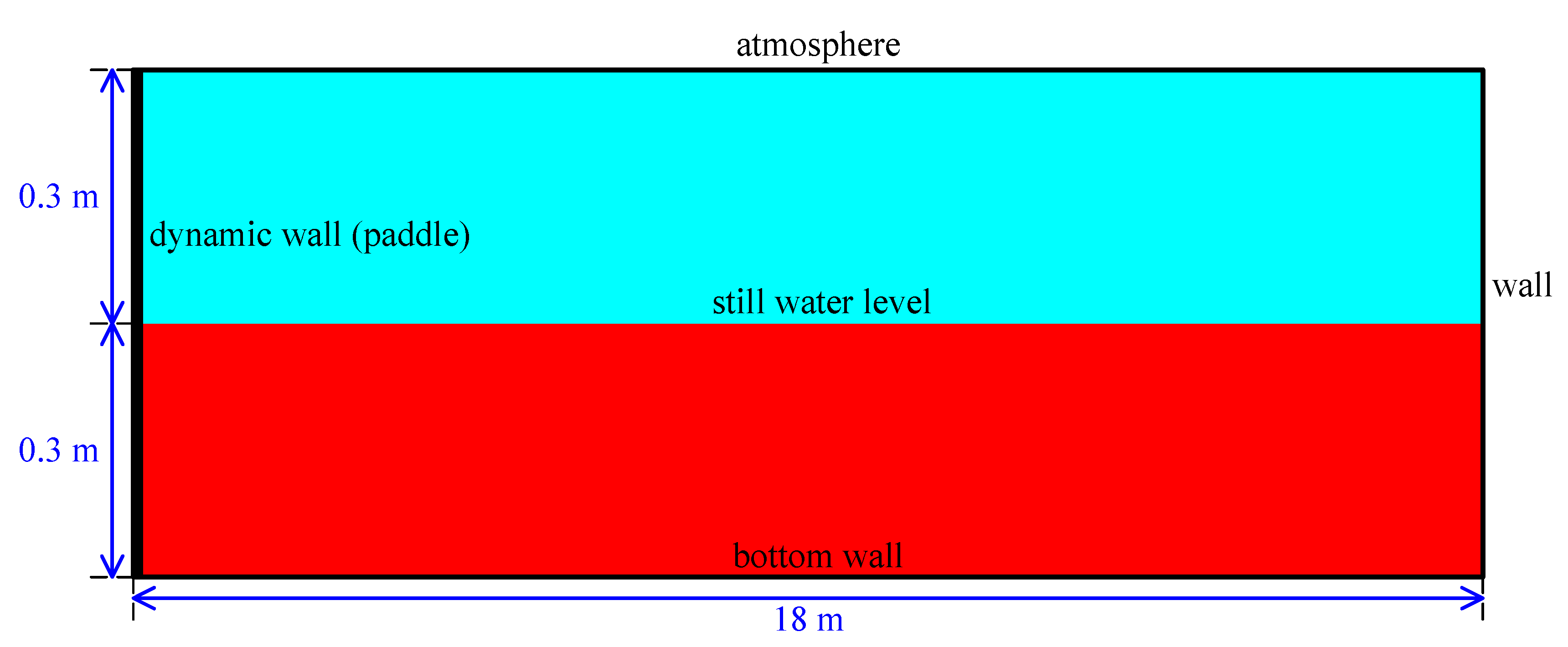
The sensitivities of wave profile to grid density and time step were investigated first. The size of the virtual wave flume is 18 m × 6 m, the water depth is 0.3 m, and the targeted wave height is 0.15 m, as mentioned. Three grids are generated by systematically doubling the number of grid points in both horizontal direction and vertical direction. There are 300 × 10, 600 × 20, and 1200 × 40 cells for the three grids.

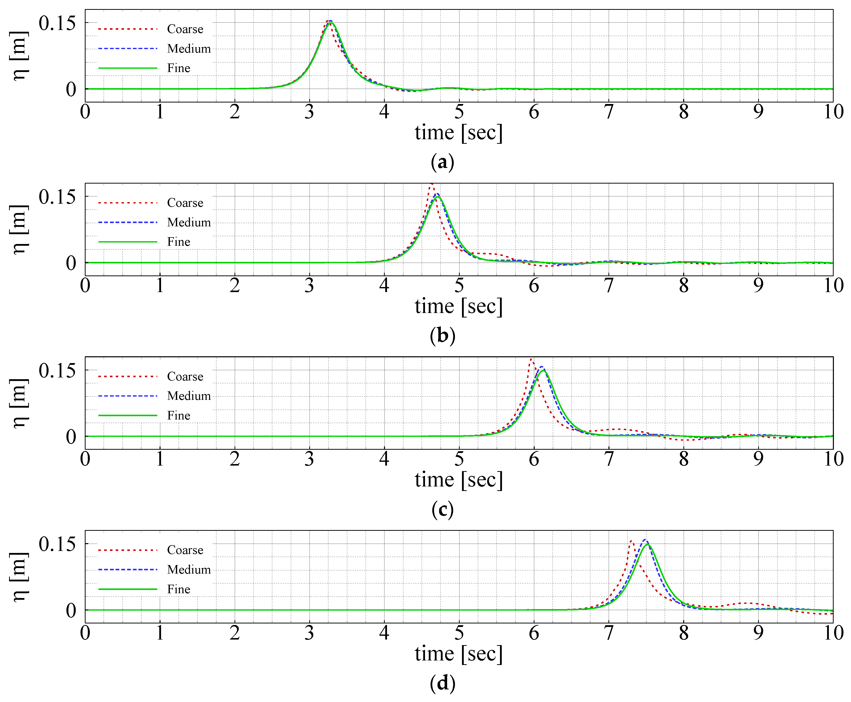
For the grid dependency analysis, the size of time step is chosen as 0.001 s. The paddle displacement used for both the grid and time-step dependency analyses are based on the ninth-order solution of solitary wave. The time traces of water surface evaluation are recorded at the positions 2, 5, 8, and 11 m during the simulations. The time traces based on the three grids are compared in Figure 5. The three time traces at x = 2 m seem closer than that at other positons, especially the leading edge of the wave. As the solitary wave propagates farther or the distance to the wave maker gets farther, the difference among the three time traces becomes larger. The maximum water surface evaluation based on the coarse grid first increases, then decreases. The time trace based on the coarse grid reaches its peak value more quickly than that based on the medium grid and fine grid, meaning that the resulting solitary wave based on the coarse grid moves faster. As increasing the grid resolution, the time trace gradually gets closer at each position, and the amplitudes of the trailing waves become smaller. When using the fine grid, the maximum water surface evaluation has been very close to the targeted one, i.e., 0.15 m, although a very slight decay of wave height is still observed at the position 11 m. The RMSE (root mean-square-error) of the grid dependency analysis is listed in

Table 2. RMSE of the grid dependency analysis.

Grid	x = 2 m	x = 5 m	x = 8 m	x = 11 m
coarse	0.0030	0.0082	0.0119	0.0137
medium	0.0013	0.0021	0.0029	0.0040
fine	-	-	-	-

.

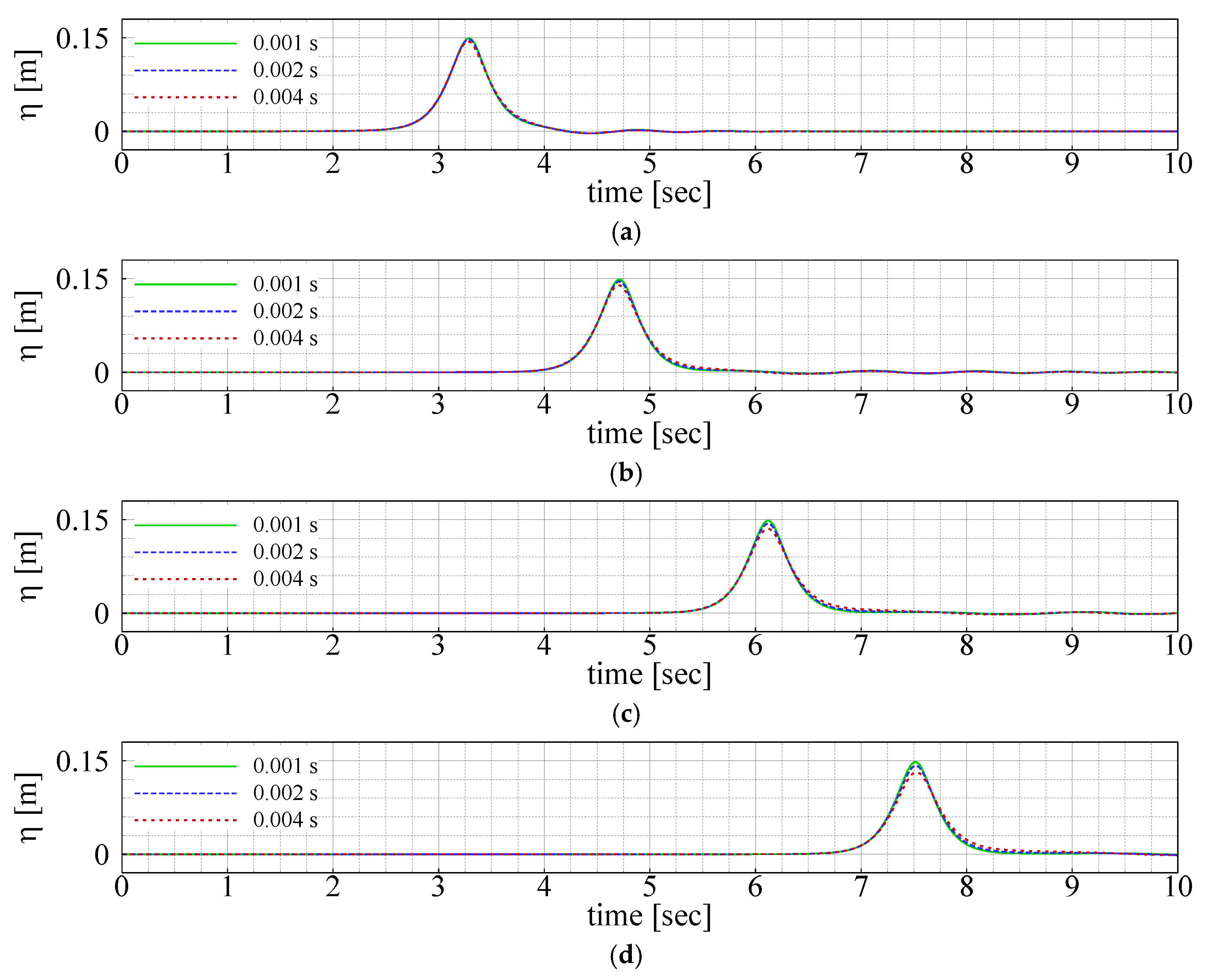
The effects of time step on the wave profile are also investigated. The fine grid is used for the investigation. Three sizes of time step, i.e., 0.001 s, 0.002 s, and 0.004 s, are taken into account. The time traces based on these time steps are compared at the positions 2, 5, 8, and 11 m as well, as shown in Figure 6. It is seen that the time step mainly affects the decay of the wave height. The wave height based on the time step size 0.004 s decreases significantly as the solitary wave propagates. However, the time traces based on the three sizes of time step at each position reach their own peak values almost at the same point in time. The time step does not influence the moving speed of the solitary wave. The RMSE of the time step dependency analysis is listed in

Table 3. RMSE of the time step dependency analysis.

Time-Step Size	x = 2 m	x = 5 m	x = 8 m	x = 11 m
0.004 s	0.0006	0.0011	0.0015	0.0019
0.002 s	0.0003	0.0006	0.0008	0.0011
0.001 s	-	-	-	-

.

Based on the dependency analyses of grid density and time step, we can see that the grid density and time-step size affect considerably the wave profile. The fine grid with 1200 × 40 cells and the time-step size 0.001 s seems to be of acceptable accuracy. Thus, this fine grid and time-step size are used for the simulations below.

5. Compare the Wave Profiles Based on the First-Order and Ninth-Order Solutions

The simulated time traces of water surface evaluation based on the first-order and ninth-order solutions of solitary wave are presented in Figure 7. The targeted wave height remains 0.15 m in the water with a constant depth of 0.3 m. The time traces at the aforementioned four positions are compared. The wave height based on the first-order solution reduces gradually as the solitary wave propagates, whereas, the loss of the wave height based on the ninth-order solution is not noticeable. As the solitary wave propagates farther, the peak value of the time trace based on the ninth-order solution gradually occurs earlier than that based on the first-order solution. This means the solitary wave based on the ninth-order solution moves faster. In addition, the amplitudes of the tailing waves based on the ninth-order solution are slightly smaller than that based on the first-order solution, which confirms the better performance of the ninth-order solution, as reported in many other publications.

6. Validation of the Numerical Results

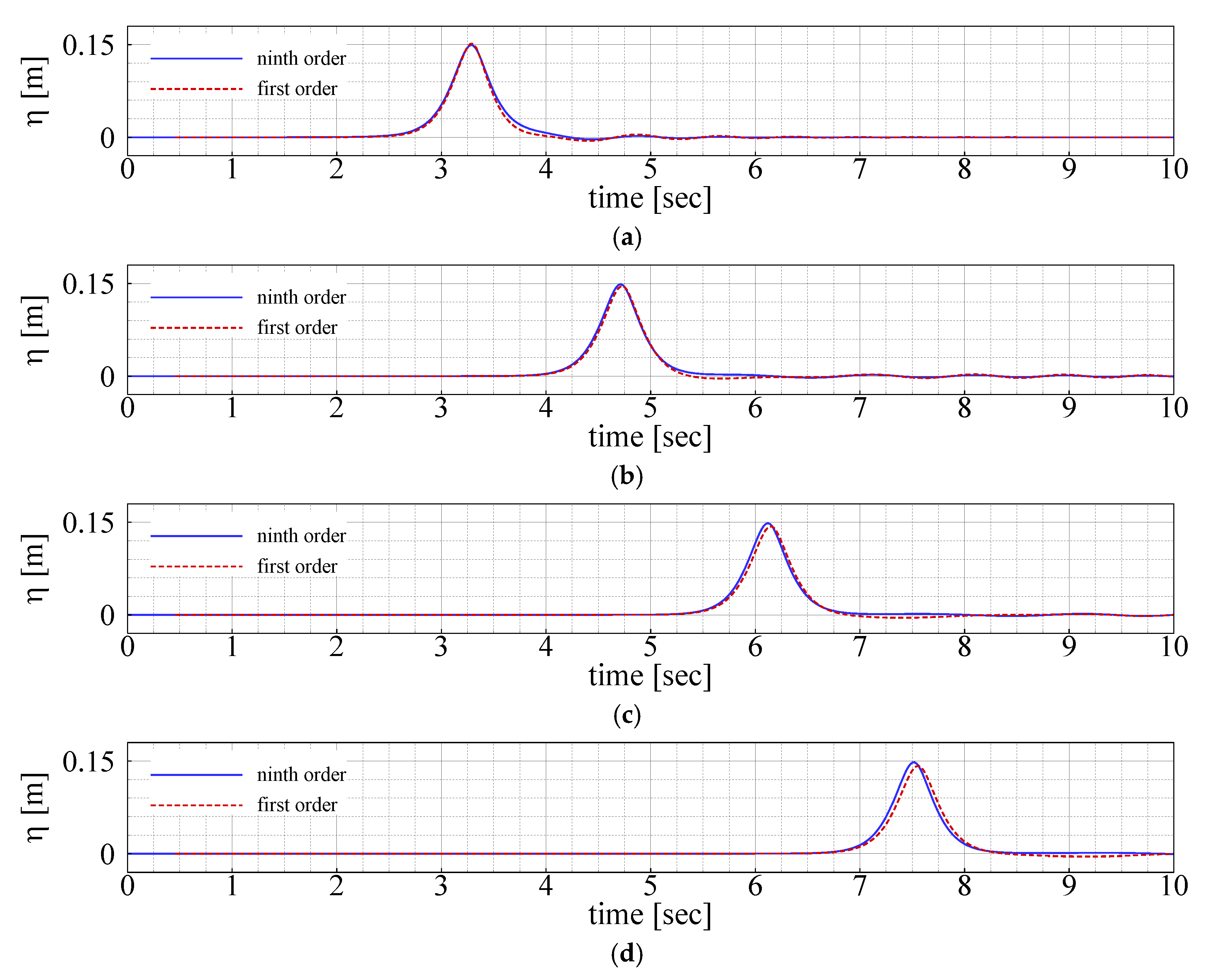
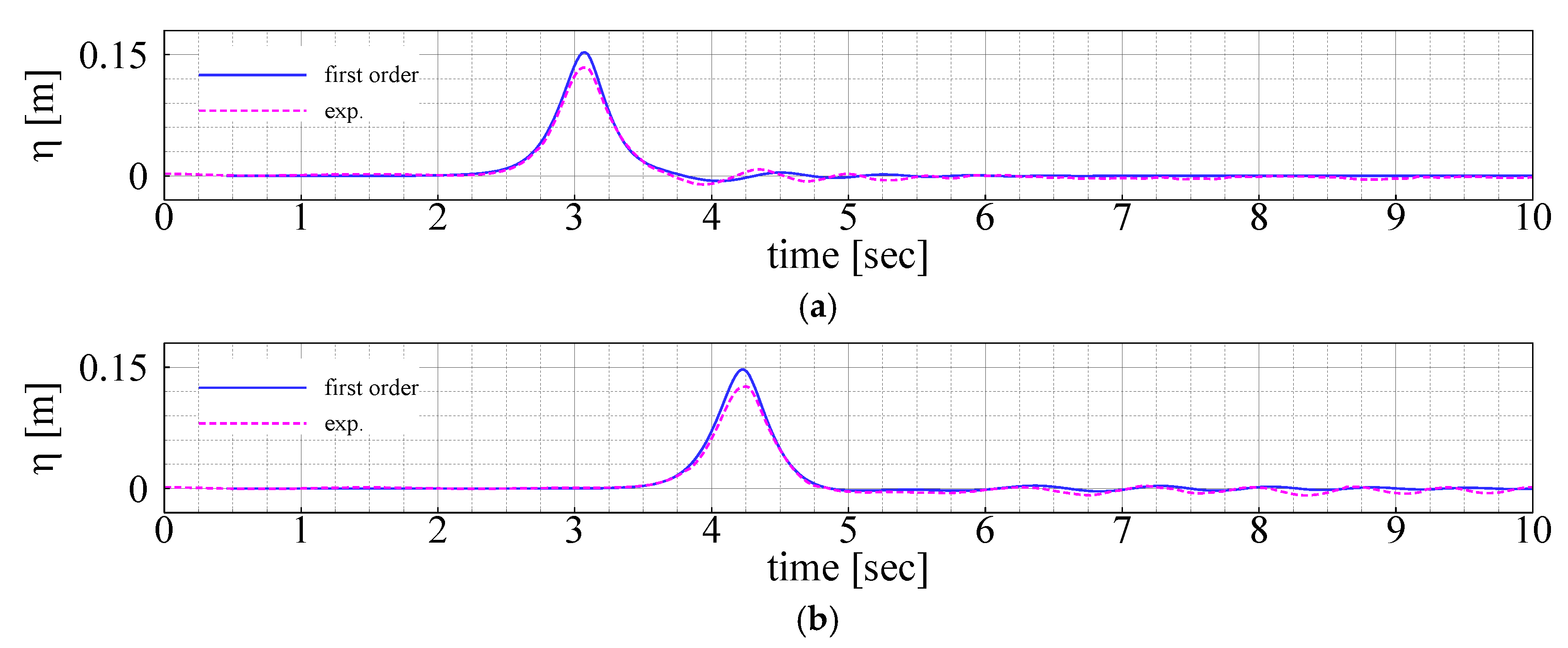
As mentioned previously, experiments were carried out at the Wuhan University of Technology to validate the present numerical method. During the experiments, the water depth was 0.3 m, and the targeted wave height was set as 0.15 m. The input paddle displacements were determined by both the first-order and ninth-order solutions of solitary waves. Two wave gauges were fixed at x = 1.55 m and x = 3.95 m to record the time histories of wave surface evaluation.

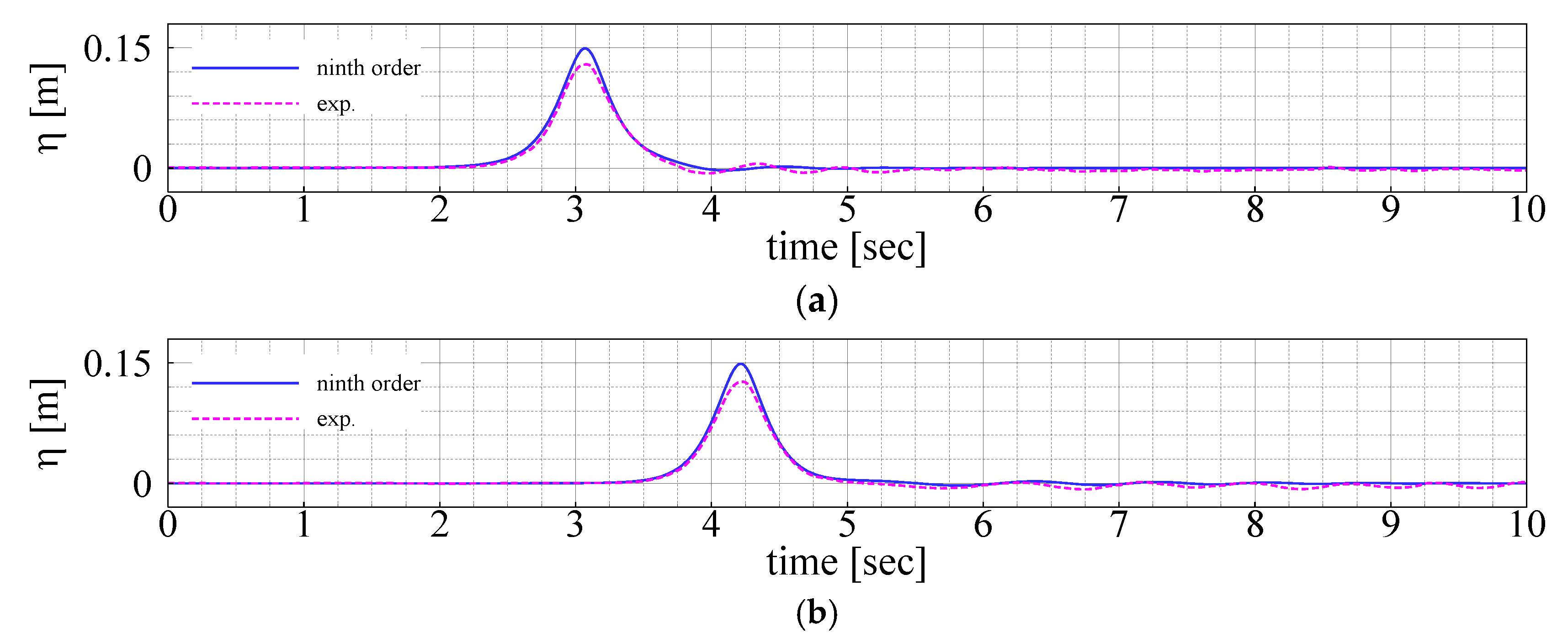
The simulated results based on the ninth-order solution are compared with the experimental data in Figure 8, while the comparisons for the results based on the first-order solution are presented in Figure 9. At first glance, all measured maximum water surface evaluations are far from the targeted one and smaller than the simulated ones. 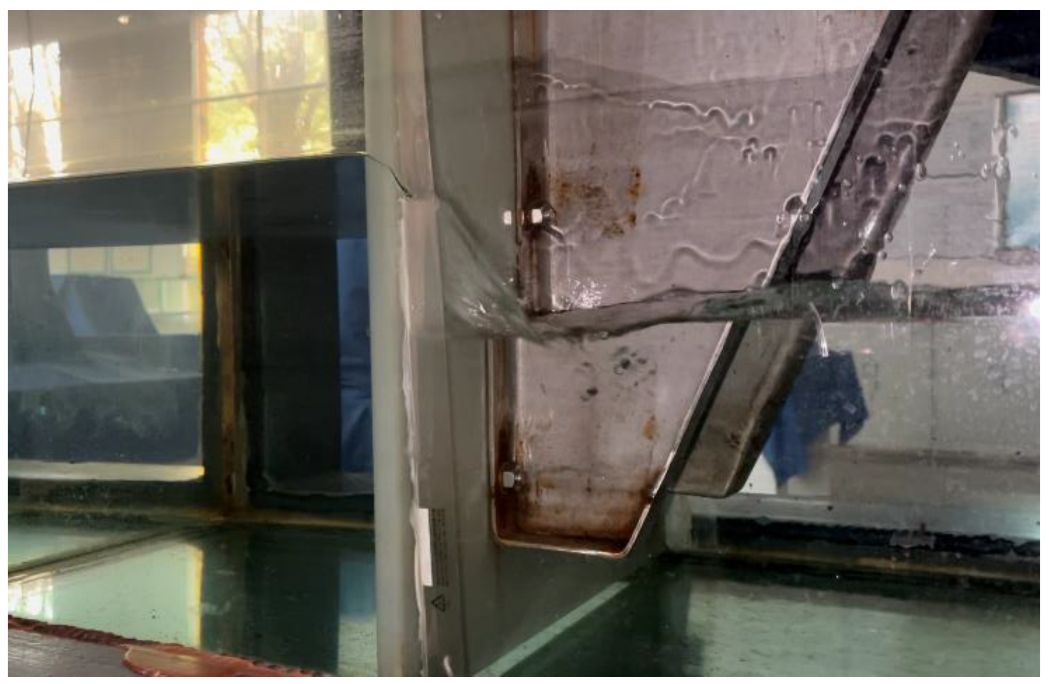The loss of wave height in experiments is around 0.02 m at x = 1.55 m, and there is a little bit larger loss at x = 3.95 m. One of the most possible reasons for this may be due to the small gaps between the paddle and flume walls. The overflow of the water through a side gap can be clearly observed when the paddle is moving forward, as shown in Figure 10. The gap between the paddle and water bottom is even bigger. However, these gaps are assumed to be closed during the numerical simulations. The simulated and measured maximum wave evaluations occur nearly at the same point in time at either x = 1.55 m or x = 3.95 m.

The measured data from Figure 8a show that after the maximum evaluation of solitary wave passes the position x = 1.55 m, the depression of the water surface at this position occurs, and afterwards the water surface elevation persistently oscillates, i.e., the trailing waves. The depression of water surface at x = 3.95 m diminishes obviously, but the oscillation of water surface elevation becomes even stronger (see Figure 8b). These phenomena are also found for the measured data based on the first-order solution of solitary waves, as shown in Figure 9; nevertheless, the depression and oscillation are a little bit more prominent. The simulated results in Figure 8 and Figure 9 display the tendencies as the same as the experimental data at either x = 1.55 m or x = 3.95 m, although the depression and oscillation are much weaker. The amplitudes of the simulated tailing waves are less than 3% of the main pulse. However, they are around 10% for the measured data.

7. Propagation Characteristics in a Step-Type Flume

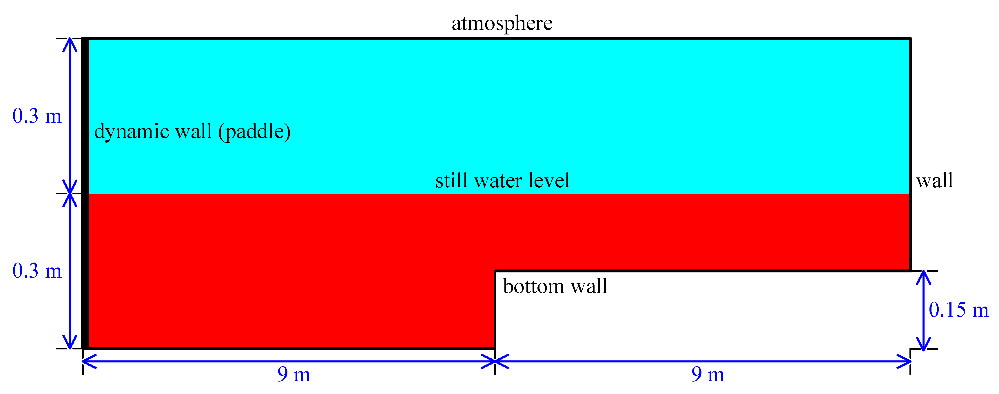
This is investigated by means of numerical simulation. Unfortunately, to conduct such an experiment is not yet possible. The solitary wave with the targeted wave height of 0.15 m is considered. The solitary wave is generated in the water with the depth of 0.3 m, and then propagates into the water region with the depth of 0.15 m. Figure 11 illustrates the computational domain. The domain length is 18 m long as well. However, a step with the height of 0.15 m locates in the middle of the flume. Actually, the computational domain with the step results from subtracting the small rectangle with a size of 0.15 m × 9 m from the domain (0.6 m × 18 m) for the case of the constant water depth, as shown in Figure 4. The small rectangle is one-eighth of that domain.

The computational grid used is very similar to the ones for the case of the constant water depth, as described in Section 3.2. There are totally 42,000 cells, i.e., 1200 × 40–600 × 10 cells, corresponding to the fine grid with 1200 × 40 cells in the Section 4. During the simulation, the size of the time step remains 0.001 s according to the analysis of time-step dependency. The time history of paddle displacement is determined by the ninth-order solitary wave solution, which is shown in Figure 2. Other numerical settings are identical to that for the case of the constant water depth.

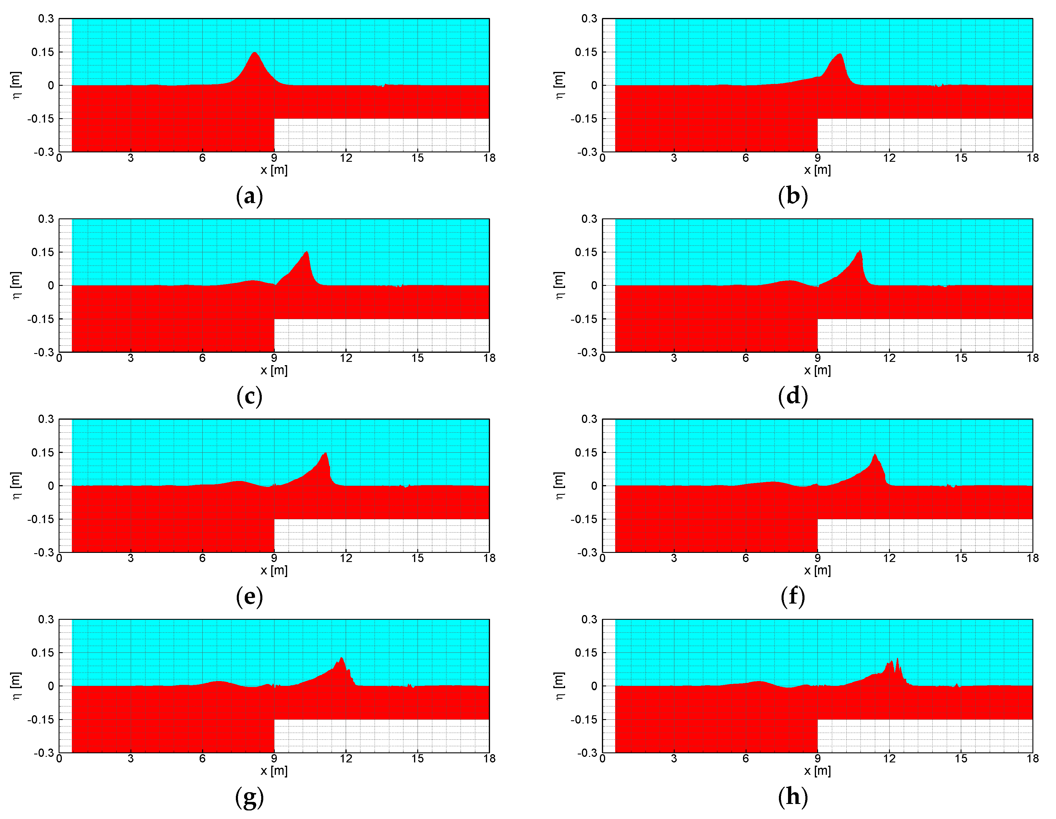
The snapshots of wave profiles at a few interesting time points are presented in Figure 12. At t = 6 s, the wave is close to but has not yet passed the step. Soon after, the wave runs past the step at t = 6.8 s, and the wave tends to split right there at the position of the step, i.e., at x = 9 m. The wave height decreases slightly at this moment. After 0.2 s, i.e., at t = 7 s, the wave completely splits into two waves. The separation point is clearly seen at the position of the step. The main wave, which enters into the shallow water and continues to move forward, becomes slimmer and its profile peak exceeds the targeted one. The other wave is due to the reflection of the step and in turn moves backward. The reflected one is much smaller than the main one. These can be observed more clearly at t = 7.2 s. As time goes on, the reflected wave keeps on moving backward. However, the main wave gradually collapses. At t = 8 s, the shape of the main wave has become indistinct. The Observations are quite similar to those reported by Gao et al. [20].

When the solitary wave propagates from the deep water into the shallow water, a part of the solitary wave is reflected because the blockage effects make the road narrower. After the main wave enters the shallow water, the moving speed of its crest looks faster than that of its trough if observing the wave profiles from t = 6.8 s to t = 7.2 s. This means that the crest loses the support of the trough so that the crest at t = 7.4 s and t = 7.6 s tends to fall down due to gravity. This leads to the collapse of the main wave.

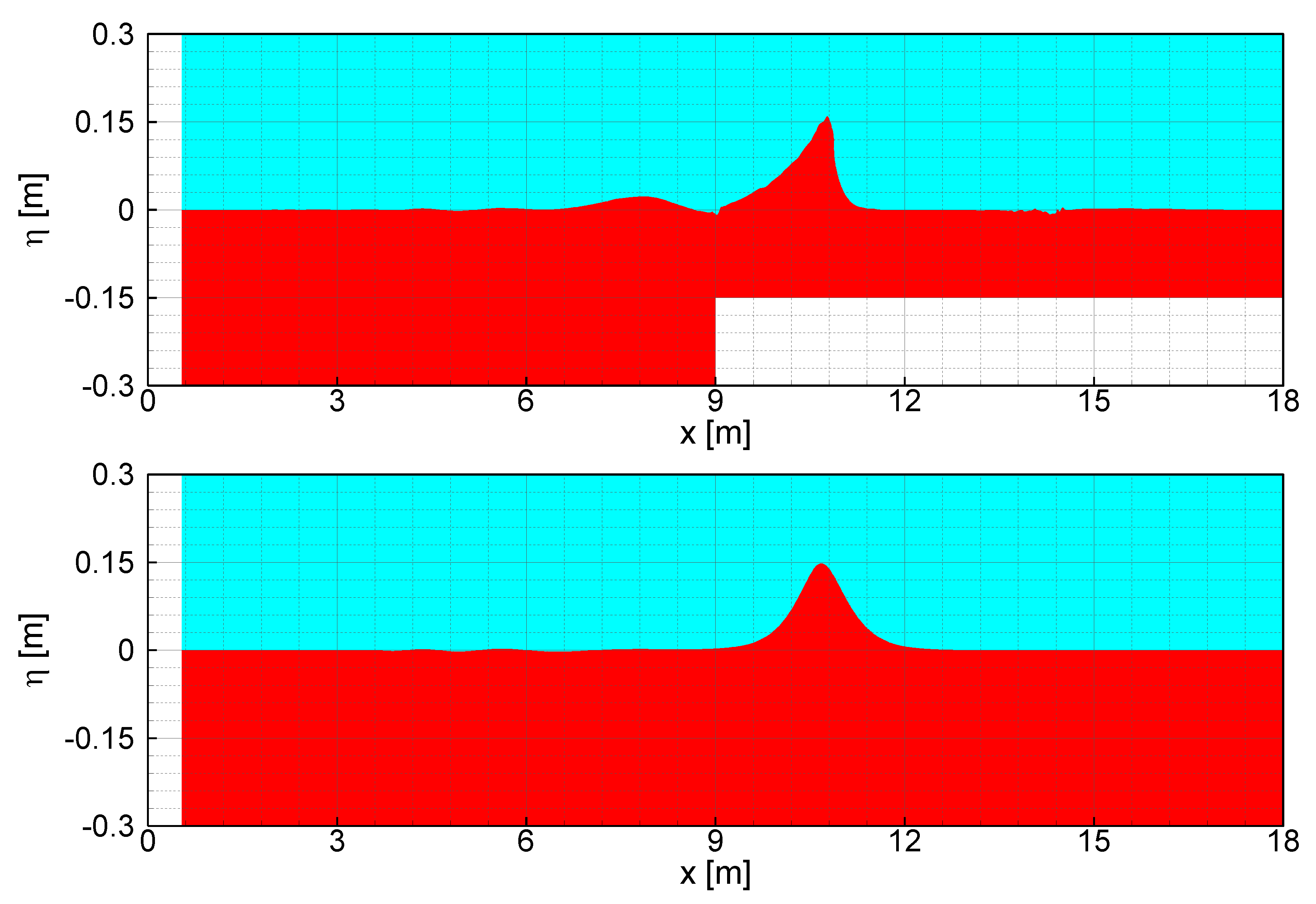
The wave profiles for the waters of constant depth and variable depth at t = 7.2 s are compared in Figure 13. As is seen, the trough of the wave in the step-type flume moves slightly slower than the trough in the water of constant depth, whereas the crest in the step-type flume moves faster. Note that the speed of the whole solitary wave (both the crest and trough) in the water with the constant depth is always consistent.

8. Concluding Remarks

This work presents a study on the generation of solitary waves by using a piston-type wave maker and the propagation characteristics of a solitary wave in a step-type flume. On the aspect of numerical simulation, one of the contributions may lie in the development of a new dynamic wall boundary condition on the platform OpenFOAM. When using this new boundary condition, the time history of the paddle displacement can be read from an input file and then used to simulate the linear motion of the paddle. In theory, it can be employed to generate any type of waves as long as the corresponding law of paddle motion is determined in advance. Experiments were also conducted for the case of water with a constant depth in order to validate the numerical results. Reasonable agreements are found between the numerical wave profiles and experimental ones.

The simulated profile of solitary waves depends greatly on the grid resolution and time-step size. Appropriate grid resolution and time step size can reduce the decay of wave height and ensure a more stable solitary wave. The better performance of ninth-order solution is confirmed when determining the paddle displacement as different than the first-order solution, e.g., the problem of wave height decay is improved.

Furthermore, the present numerical method could be expanded to generate waves in a three-dimensional wave tank. The hydrodynamic analyses of solid structures in solitary waves, especially in a more realistic water area topography, could be performed in the future. This might promote the understanding of the destructive effects of solitary waves offshore or nearshore structures.