Numerical Simulation on the Local Scour Processing and Influencing Factors of Submarine Pipeline

Abstract

To investigate the different influencing characteristics of local scour around submarine pipelines, hydrodynamic and sediment transport two-dimensional models based on Flow-3D are used to numerically simulate the local scour around the pipeline under steady currents. An RNG k-ε turbulence model is applied to simulate the turbulent flow field around the pipeline. The instantaneous shear stress of the bed surface is taken as the starting and transporting conditions of the sediment. The simulation results of the equilibrium scour depth and terrain around the pipeline are verified with the previous experimental results, which perform with good agreement. Then, the numerical simulation method is applied to investigate the local scour process around the pipeline. The results show that shear stress is the main driving force of scour around a pipeline. The velocity, sediment grain size, pipeline diameter, and the initial gap between the pipeline and the seabed, significantly affects submarine pipeline equilibrium scour depth and terrain in varying degrees.

1. Introduction

With the unceasing progress of science and technology and the continuous depletion of land resources, human’s exploitation of energy has gradually developed into the ocean. Submarine pipeline is of great importance to transport submarine resources, which takes on the arduous and difficult task of transporting oil, natural gas, and other energy sources. As the exploitation of marine resources increase, more and more pipelines have been laid under the sea. However, at the same time, submarine pipelines are also confronted with potential threats from the appalling environment. Waves and currents result in the movement of sediment around the pipeline, and with the transporting of sediment, obvious scour pits will form beneath the pipeline. With the development of scouring, the pipeline will gradually sag, which will generate stress concentration, and eventually lead to a fatigue fracture. Therefore, it is necessary to study and explore scour around pipelines.

Experimental research and the numerical calculation of pipeline local scour have been implemented by many researchers. Kjeldsen et al. [1] conducted local scour tests on pipelines and found that the equilibrium scour depth mainly depended on the pipeline’s geometry and flow velocity. Ibrahim and Nalluri [2] divided the local scour of pipelines into clear water and live bed scour in their experiments, and presented a scour depth prediction formula under different conditions. Mao [3] studied the interaction mechanism between the pipeline and the seabed through laboratory experiments. Chiew [4] investigated Mao’s research and considered that piping is the primary cause of the initiation of scour. Li and Cheng [5] used a numerical simulation method to analyze the flow field pattern and local scour pattern around submarine pipeline under a unidirectional current. Brørs [6] applied the k-ε turbulence model and an adaptive finite element mesh to simulate the flow field and local scour around the pipeline. Moncada-M and Aguirre-Pe [7] experimentally investigated pipeline scouring in rivers and proposed a formula to calculate the equilibrium scouring depth. Liang et al. [8] numerically simulated the local scouring of submarine pipelines in a unidirectional current. Dey and Singh [9] constructed a laboratory scaled model to evaluate scouring depth in river conditions. Cheng and Zhao [10] used the finite volume method to solve the Navier-Stokes (N-S) equations of unsteady flow, and a k-ω turbulence model to simulate the pipeline scour. Etemad-Shahidi et al. [11] investigated the wave-induced scouring depth under submarine pipelines with a model tree method. Azamathulla and Zakaria [12] predicted the scour below a submerged pipeline by using an artificial neural network. Najafzadeh et al. [13] implemented a group method of data handling to predict the pipeline scour depth in clear water and in live bed conditions. Zhao et al. [14] researched the scour depth and time scale of parallel pipelines with different gap to diameter ratios through numerical simulation. Zhang et al. [15] experimented on tandem pipelines’ scour under live bed and clear water conditions. Zhang et al. [15] numerically studied the effects of the gap to diameter ratio on local scour and the vortex-induced vibration of the pipeline. Zhao et al. [16] studied the scouring mechanism of a piggyback pipeline under the action of a unidirectional current via experiments and numerical simulation. Ajdehak et al. [17] numerically investigated the local scour formation of a sagging subsea pipeline in steady currents. Zang et al. [18] studied the scour development and time scale of a partially buried pipeline under an oblique current and waves. Parsaie et al. [19] predicted the scour depth beneath a pipeline with a support vector machine. Hu et al. [20] investigated the effects of G/D and flow velocity on scour depth through numerical simulation. Hu et al. [21] applied a backpropagation neural network optimized by a genetic algorithm to predict the scour depth of submarine pipelines. Li et al. [22] studied parallel pipeline scour with different gap ratios under wave-plus-current conditions. Nevertheless, few studies have analyzed the depth and terrain variation of local scour processes in submarine pipelines considering different influencing factors. In this paper, a numerical simulation model is established to investigate the local scour process of submarine pipelines on shear stress, velocity field, scour depth and terrain under steady currents. In addition, the effects of velocity, sediment grain size, diameter, the initial gap between the pipeline and the seabed, and the pipeline’s distance, for submarine pipelines are discussed in detail.

2. Numerical Methods

The commercial software Flow3D is used to investigate the local scour around pipelines. The volume of fluid (VOF) method is adopted to track the free water surface. The model utilizes the Fractional Area/Volume Obstacle Representation (FAVOR) method to model complex geometric regions in fixed rectangular meshes.

2.1. Continuity Equations

In Cartesian coordinates, the flow field is obtained by solving the N-S equations for incompressible fluid and the renormalization group (RNG) k-ε turbulence model. 2.1. Continuity equations of fluid can be expressed as [23]:

$$\frac{\partial (U{A}_x)}{\partial x}+\frac{\partial (V{A}_y)}{\partial y}+\frac{\partial (W{A}_z)}{\partial z}=0$$

(1)

where U, V, W are the three-dimensional velocity components and A_x, A_y, A_z are the fractional areas open to flow in the x, y and z directions, respectively.

2.2. The Turbulence Model

This research uses the RNG k-ε turbulence model, which is composed of a standard k-ε model correction. The turbulent kinetic energy transport equation may be expressed as:

$$\frac{\partial k_T}{\partial t}+\frac{1}{V_F}(U{A}_x\frac{\partial k_T}{\partial x}+V{A}_y\frac{\partial k_T}{\partial y}+W{A}_z\frac{\partial k_T}{\partial z})=P_T+G_T+Dif{f}_T-{\epsilon }_T$$

(2)

Turbulent kinetic energy dissipation equation:

$$\frac{\partial k_T}{\partial t}+\frac{1}{V_F}(U{A}_x\frac{\partial {\epsilon }_T}{\partial x}+V{A}_y\frac{\partial {\epsilon }_T}{\partial y}+W{A}_z\frac{\partial {\epsilon }_T}{\partial z})=\frac{CDIS1\cdot {\epsilon }_T}{k_T}(P_T+CDIS3\cdot G_T)+Dif{f}_{\epsilon }-CDIS2\frac{{\epsilon }_T^2}{k_T}$$

(3)

where V_F is the volume fraction, G_T is the turbulent energy term generated by buoyancy, P_T is the kinetic energy generated by the velocity gradient, k_T is the turbulent kinetic energy, ε_T is the turbulent energy dissipation rate, CDIS1, CDIS2 and CDIS3 are all dimensionless adjustable parameters, which have defaults of 1.44, 1.92 and 0.2; Diff_ε is the diffusion of dissipation.

2.3. Sediment Transport Model

In this research, the sediment is assumed to be non-viscous. The particle size, density, critical repose angle and critical Shields parameters are taken into account in the sediment model.

The dimensionless critical Shields parameter is computed using the equation [24]:

$${\theta }_{cr}=\frac{0.3}{1+1.2d_{\ast }}+0.055[1-\exp (-0.02d_{\ast })]$$

(4)

$$d_{\ast }=d_{50}{[\frac{{\rho }_f({\rho }_s-{\rho }_f)g}{{\mu }^2}]}^{\frac{1}{3}}$$

(5)

where, d₅₀ is the median sediment particle diameter, ρ_f is the fluid density, ρ_s is the density of the sediment, μ is the dynamic viscosity of fluid, and g is the magnitude of the acceleration of gravity.

The critical Shields parameter can be modified for sloping surfaces to include the angle of repose. The modification further alters ${\theta }_{cr}^{\prime }$:

$${\theta }_{cr}^{\prime }=\frac{{\theta }_{cr}(\cos \phi \sin \beta +\sqrt{{\cos }^2\beta {\tan }^2\phi -{\sin }^2\psi {\sin }^2\beta })}{\tan \phi }$$

(6)

where β is the angle of the bed slope, φ is the angle of repose for the sediment (default is 32°), ψ is the angle between the flow and the upslope direction.

The entrainment lift velocity of the sediment is then computed as [25]:

$$u_{lift}=\alpha n_s{d}_{\ast }^{0.3}{(\theta -{\theta }_{cr})}^{1.5}\sqrt{\frac{d_{50}({\rho }_s-{\rho }_f)g}{{\rho }_f}}$$

(7)

where n_s is the outer normal vector perpendicular to the sedimentary mass and α is the starting parameter. The setting velocity equation proposed by Soulsby [24] is used:

$$u_{setting}=\frac{v_f}{d_{50}}[{({10.36}^2+1.049d_{\ast }^3)}^{0.5}-10.36]$$

(8)

where v_f is the kinematic viscosity of fluid.

The empirical formula proposed by Meyer-Peter and Müller [26] is used for the bed-load transport equation. The formula is as follows:

$$q_b=b{(\theta -{\theta }_{cr}^{\prime })}^{\frac{3}{2}}{[g(\frac{{\rho }_s-{\rho }_f}{{\rho }_f})d_{50}^3]}^{\frac{1}{2}}$$

(9)

where b is a coefficient, typically equal to 8, q_b is the volumetric bed-load transport rate.

The suspended sediment concentration is calculated by solving the transport equation:

$$\frac{\partial C_s}{\partial t}+\nabla \cdot (u_s{C}_s)=\nabla \cdot \nabla (E{C}_s)$$

(10)

where C_s, E and u_s are the suspended sediment mass concentration, diffusivity and suspended sediment velocity, respectively.

2.4. Boundary Conditions

Figure 1 displays the boundary conditions of the numerical simulation model. The top of the model is defined as the pressure boundary, which is the standard atmospheric pressure, and the free surface of the fluid is captured by the volume of fluid method. As for the bottom boundary, the wall boundary condition is set. In addition, symmetric boundary conditions are defined for the front and back of the model. The inlet flow of the numerical model is set as the specified velocity and the outlet flow of the model is defined as the outflow boundary.

3. Validation Models

To verify the accuracy of the numerical model, a validation of the sediment scour model between the present model and previous experimental results (Mao (1987)) is carried out in this section. The experiment was performed in a flume with a reduced scale pipeline model (D = 10.1 cm). The surface of the pipeline was hydraulically smoothened. The channel was 23 m long and had a rectangular cross section of 2 m wide and 0.5 m deep, which contained an 8 m long and 15 cm deep layer of sediment with a mean particle diameter of 0.36 mm. The experiment was run with inflow velocities of 0.4 m/s and 0.35 m/s, respectively, for live bed and clear water conditions.

Figure 2 and Figure 3 illustrate the validation of the scour terrain and depth around the pipeline at the equilibrium stage. A good agreement with the experimental results proposed by Mao (1987) was obtained from the numerical model. Under both conditions, the experimental local scour depth increased rapidly at the initial stage of scour development, and then increased slowly until the equilibrium state was reached. For the numerical model, the scour depth increased slightly faster than the experimental results in the scour development stage, but during the rest of the calculation time, it was in good agreement with the experimental results. The equilibrium scour depth that was achieved from the present model was 2.3% larger than the experimental model for clear water and 6.7% larger for the live bed condition. From the shape of the scour terrain, the pipeline scour terrain was similar to the test conditions. Overall, the above validations indicate that the presented model is capable of studying the process of pipeline local scour.

This numerical simulation mainly focuses on the flow field and seabed bed surface changes near the submarine pipeline. The grid domain is shown in Figure 4, which is divided into two parts. The first part is the flow development part, and the second part is the sediment scour. For the first part of the grid, the seabed is set as non-scour. The length in the x direction is set as 50D, the length in the z direction is set as 6.5D, in which D is the pipeline’s diameter. The grid size is 0.01 m and the number of grid blocks is about 32,500. Then, for the sediment scour grid, the pipeline contacting the seabed is partially refined. The maximum grid of far from the pipeline is 0.01 m, and the minimum grid of near the pipeline and the bed is 0.005 m. The length in the x direction is set as 30D, and the number of grid blocks is about 19,500.

In order to eliminate errors caused by the quantity of grids in the calculation process, the grid’s independence from the numerical model was verified. Three kinds of grid refinement with the same quality and different sizes were used to simulate the live bed scour test of Mao’s experiment. The results are shown in

Table 1. Mesh grid.

Total number of grids	41,000	52,000	67,600
Scour depth	0.0642 m	0.0621 m	0.0618 m
Time	75,200 s	88,490 s	124,270 s

. With the increase in mesh grid number, the scour depth was similar to the applied test mesh, whereas the decrease in the mesh grid number caused the great difference in scour depth. The variation amplitude of the scour depth calculated by the refinement mesh sizes was small, which meets the requirement of grid independence. Considering the accuracy of the numerical simulation and the calculation’s time cost, a mesh number of 52,000 was selected for the calculation.

4. Numerical Results and Discussion

The main purpose of this research is to investigate the process of local scour and influencing factors around pipelines. As shown in

Table 2. Parameters of the model.

Parameters	v	D	d50	e/D	ρ	ρs
Value	0.4 m/s	0.15 m	0.4 mm	0	1000 kg/m3	2650 kg/m3

, the specific parameters were as follows: The pipeline diameter was D = 0.15 m. The lengths of the upstream and downstream sediment beds were 2 m and 1 m, respectively. The depth of the water was 0.5 m, which had no significant effect on the numerical results. In addition, the depth of the sediment bed was 0.15 m. The median particle diameter of the sediment d₅₀ was 0.4 mm and its density ρ_s was 2650 kg/m³. The velocity was v = 0.4 m/s and the initial gap between the pipeline and the seabed ratio was e/D = 0, which means the pipeline was bottom-seated on the seabed. After specifying the sediment’s scour parameters and other physical properties, the numerical model could be studied in detail.

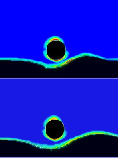
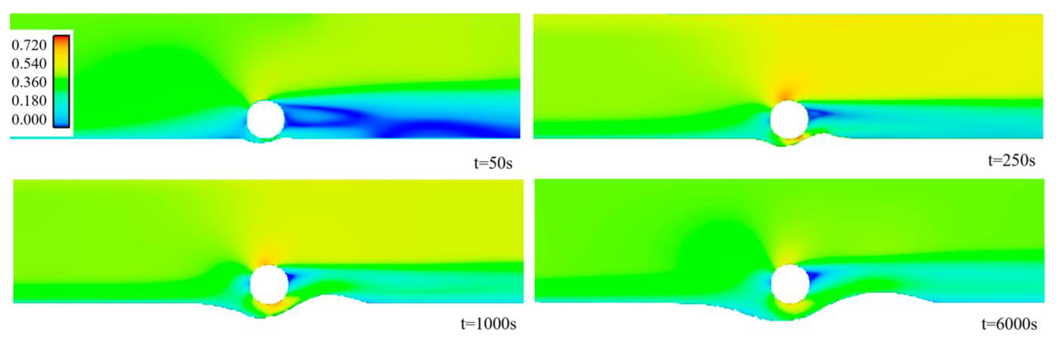
4.1. Process of Scour

Figure 5 illustrates the process of pipeline scour and suspension under steady currents, which can be divided into three stages: 1. Clearance scour: Due to the pressure difference between the upstream and downstream sections of the pipeline near the bed’s surface, the seepage phenomenon occurs below the pipeline. The gap, which is much smaller than the pipeline’s diameter, between the pipeline and the seabed is gradually generated and extended upward and downstream. As shown in Figure 5, the scour profile increases rapidly along the development of the scour tunnel (t = 50 s and t = 250 s), and the accumulated dune is formed downstream of the pipeline. 2. Wake scour: When the gap between the pipeline and the seabed increases to a certain value (t = 1000 s), the development of the scour terrain slows down in front and below the pipeline, but the dune behind the pipeline continues to change in the downstream direction. Because of this, the flow velocity in front of the pipeline tends to be stable, while the sediment is deposited at the rear of the pipeline due to vortex shedding. 3. Equilibrium scour: When the depth of the scour under the pipeline reaches a balanced stage (t = 6000 s), the scour around the pipeline is no longer strong compared to the wake scour stage, the scour terrain extends in two directions, and the mound downstream of the pipeline becomes larger and moves backward. After that, the shape of the bed surface no longer changes, and at this time, it is considered that the scour has stabilized and reached an equilibrium state.

When the shear stress of the sediment particles is greater than the critical shear stress τ_c, the sediment particles will be moved away, and the uplift force of the sediment is greater than the force impeding the uplift. On the contrary, when the shear stress near the bed’s surface is less than the critical shear stress, the flow will not be able to cause the sediment to move. The critical shear stress of the sediment particles in Flow-3D can be calculated by the critical Shields number θ_c, and the instantaneous shear stress can be calculated by the turbulent dynamic energy method, which can be expressed as:

$$k=0.5(\overline{u^{\prime 2}}+\overline{v^{\prime 2}}+\overline{w^{\prime 2}})$$

(11)

$$\tau =c\rho k$$

(12)

where, u′², v′², w′² represent the fluctuating velocity of horizontal x, transverse y and vertical z near the bed surface, respectively, c is a constant, generally to 0.19, and ρ is water density (Hirt and Nichols, 1988). Flow-3D introduces sheer stress excess in post-processing, which can be expressed as:

$${\tau }_e=\tau -{\tau }_c$$

(13)

where, τ_e is shear stress excess, τ is instantaneous shear stress, and τ_c is critical shear stress. When the shear stress excess is greater than zero, the seabed will be scoured. With the scour terrain expanding, the bed surface’s shear stress will decrease, and when the shear force excess is less than zero, the seabed sediment will no longer move.

As can be seen from Figure 6 and Figure 7, when the tunnel is first formed, the shear stress excess in the tunnel increase rapidly to 0.85 Pa (t = 50 s) due to the influx of water; meanwhile, the velocity reaches to 0.47 m/s. At the initial development of scouring, due to the small tunnel occurring between the pipeline and the sediment bed, a large amount of water rushes out from the bottom of the pipeline. The shear force at the bottom of the pipeline and the bed increases in a short time, so the shear stress of the sediment bed’s surface exceeds the sediment incipient shear stress, the sediment transport volume in the tunnel increases greatly, and the scour terrain increases rapidly along the whole direction of the scour hole. At t = 250 s, the maximum shear stress excess on the bed surface at the lower rear area of the pipeline is 3.43 Pa, and the maximum velocity is 0.72 m/s. The maximum shear stress excess and the maximum velocity is located at the lower right side of the pipeline in Figure 6 and Figure 7. In addition, the velocity distribution is similar to the shear stress excess distribution. As the scour terrain expands and the distance between the pipeline and the seabed surface increases, the shear stress excess of the bed surface decreases rapidly in most areas, which is still greater than 0. This means that scour is still happening. The maximum shear stress excess of the bed’s surface appears on the incident flow surface of the sand dune, but the strength is getting weaker, and the stresses of the bed tend to balance. Meanwhile, the maximum flow velocity point is moving from the lower right side to directly below the pipeline. Finally, due to the development of scour, the depth and terrain of the scour expands unceasingly, in the case of equal incoming flow velocity; as the distance between the bed surface and the pipe increases, the shear stress excess decreases with this development, and the sediment carrying ability of the flow decreases. The fixed trailing vortex behind the pipeline, with the influence of gravity and bed friction, causes sediment deposition downstream of the pipe. In addition, the slope formed by sand deposition downstream of the pipeline increases the sediment critical shear stress on the piping downstream of the sand dunes, forming a slope, which makes the critical shear stress increase. The shear stress excess of the bed tends to be 0, and the bed surface is difficult to change, and there is almost no interaction between the pipeline and the bed’s surface. Once the bed’s shear stress is close to or less than the critical shear stress, the scour terrain may not develop anymore. At this time, the maximum flow velocity point of the pipeline is located directly below the pipeline. This is consistent with the development of the scour process, which indicates that the shear stress is the main driving force of scour around the pipeline.

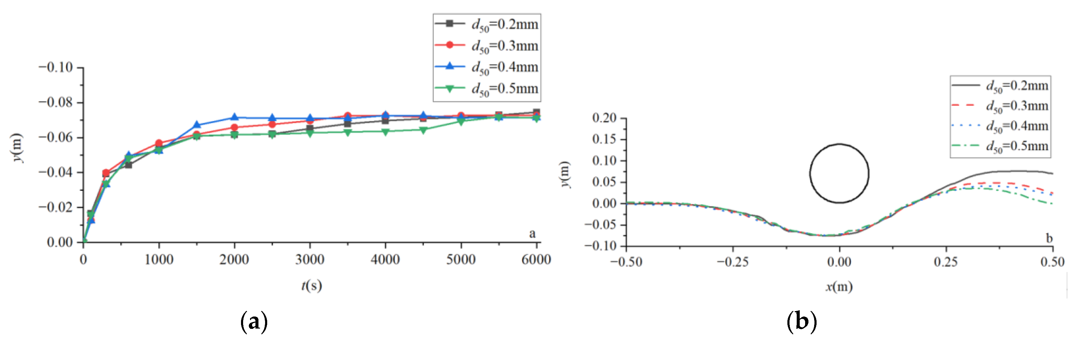
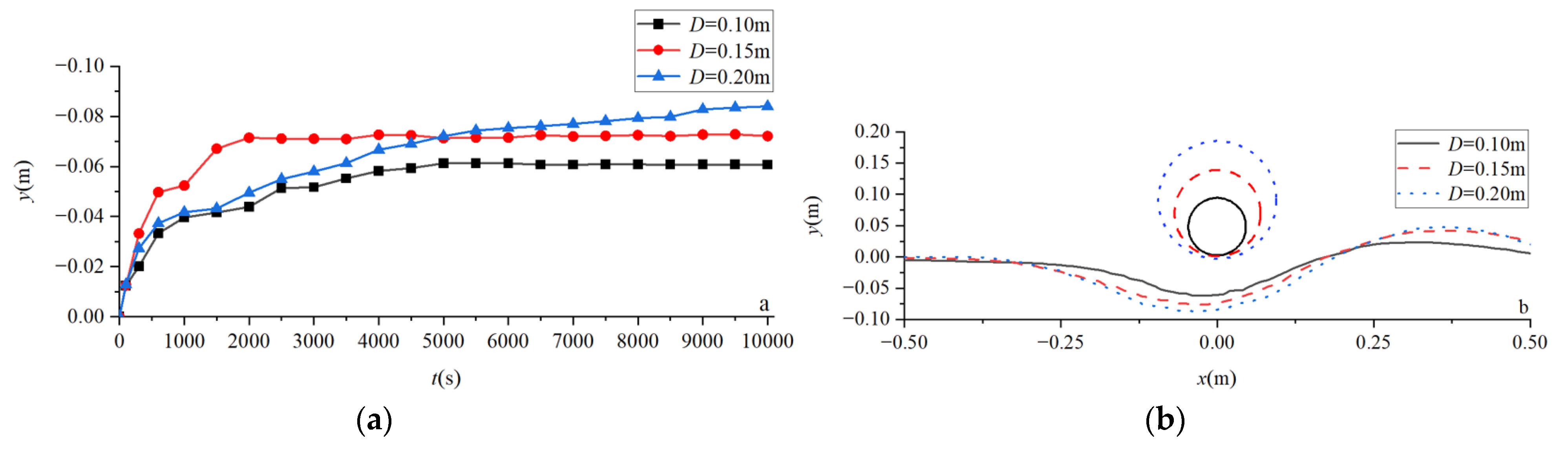
4.2. Scour Depth and Terrain under the Influence of Multiple Factors

To further study the scour process around the submarine pipeline, the influence of related parameters on the scour depth and terrain development process is further discussed by adjusting the flow rate, sediment mean diameter, pipeline diameter, and the distance between the pipeline and the seabed in the model.

Figure 8 illustrates the development of the scour depth and equilibrium in the scours terrain considering v = 0.28, 0.34, and 0.46 m/s, respectively. Other parameters are the same as the Table 2 settings. The variation of scour depth under a different flow velocity is shown in Figure 8a. Both of the test models increase rapidly in the early stage of scour, but the scour rate slows down with time development, and basically, reaches the equilibrium scour depth at 2000 s. In the case of v = 0.28, 0.34, 0.40 and 0.46 m/s, the equilibrium scour depth under the pipeline is 0.049, 0.062, 0.072 and 0.079 m, respectively. Figure 8b shows the comparison results of the scour terrain under different velocities. Velocity has a significant impact on the local scour of pipelines, and the equilibrium scour depth and the range of scour terrain under the pipeline gradually increase and expend with the increased velocity. Downstream of the pipeline, the deposition mound becomes larger, due to the increased velocity.

Figure 9 shows the local scour of pipeline when the median sediment particle size d₅₀ = 0.2, 0.3, 0.4 and 0.5 mm, respectively. Other parameters are the same as the Table 2 settings. Figure 9a shows the variation in the maximum scour depth under the pipeline with time under the condition of different sediment diameters. The variation of scour depth is similar, and there is little difference in scour depth under different sediment sizes, which means that sediment size has little effect on scour depth. However, as the sediment size becomes smaller, the scour depth becomes deeper. As shown in Figure 9b, at the same velocity, the smaller the sediment mean diameter, the smaller the critical shear force required to initiate, and the higher the sediment transport rate. Therefore, in the case of d₅₀ = 0.2 mm, the sedimentary mound and the influence area of sediment accumulation behind the pipeline is larger than the other cases. The scour depth under the pipeline gradually decreases with the increase in d₅₀, because the smaller the median particle size of the sediment, the easier it is to scour.

Figure 10 shows the local scour depth and terrain of the pipeline when the pipeline diameters D = 0.1,0.15 and 0.2, respectively, with the same settings of the other parameters as shown in Table 2. With the increase in the pipeline’s diameter, the scour depth below the pipeline decreases. When the pipeline’s diameter is 0.2 m, the scour development trend is different; the time delay for the scour depth to reach equilibrium under a larger pipeline diameter, and the development of scour in the early stage, is not faster than the other models due to the obstruction of water flow by the larger pipeline’s diameter, but because the increase in the pipeline’s diameter leads to an increase in scour depth equilibrium. Figure 10b illustrates the effect of the pipeline’s diameter on scour terrain equilibrium. The larger pipe diameter has a greater influence on the bed’s surface, which makes the change in the scour terrain wider and the change in the seabed more intense.

Figure 11 shows the local scour depth and terrain of the pipeline when the initial gap ratio between the pipeline and the seabed e/D = 0, 0.1, 0.3 and 0.5, respectively, with the same settings for other parameters as shown in Table 2. From Figure 11a, with the increase in the initial gap, the scour depth below the pipeline decreases. Meanwhile, the time for the scouring to reach equilibrium is also decreasing. As the distance between the bed’s surface and the pipeline increases, the interaction is weakened and the flow field and shear stress near the bed’s surface are more likely to reach an equilibrium state. As shown in Figure 11b, under a different initial gap, the scour terrain below the pipeline is different, but the sediment accumulation’s height and range downstream of the pipeline are basically the same. This is because, when the bed’s surface near the pipeline reaches equilibrium, the shear stress excess of the bed is similar downstream of the pipeline, which causes a similar shape in the deposition mound.

5. Conclusions

The local scour around pipelines under a steady current is numerically studied. Based on the numerical results, the following conclusions can be obtained.

Two-dimensional submarine pipeline scour models were established under a steady current selecting the RNG k-ε turbulence model to solve the flow field around the pipeline, the FAVOR method to accurately describe the shape of the pipeline, and the Tru-VOF method to track the change in the water–sand interface with the scour pattern. The experimental results from Mao (1987) for live bed and clear water conditions were employed to verify the calculations’ accuracy and the reliability of the numerical model.

The process of pipeline scour can be divided into clearance scour, wake scour and equilibrium scour. In addition, the shear stress caused by high velocity in the tunnel between the pipeline and the bed causes scour development, which is the main driving force of scour terrain formation. The fixed trailing vortex behind the pipeline, with the influence of gravity and bed friction, causes sediment deposition downstream of the pipe. Once the bed’s shear stress is close to or less than the critical shear stress, the scour terrain may not develop anymore.

The scour depth equilibrium between the submarine pipeline and the terrain is influenced by the velocity, sediment diameter, pipeline diameter, and the initial gap between pipeline and bed, in varying degrees. Velocity has a significant effect on the scour depth, and the scour depth increases with the increase in velocity. Reducing the flow rate near the pipeline helps to reduce and avoid local scour. The change of sediment diameter has little effect on scour depth; however, the scour depth deepens with a larger sediment size. The shear stress excess of the seabed is positively associated with velocity and negatively associated with sediment diameter. A larger pipe diameter has a greater influence on the bed’s surface, which makes the change in scour topography wider and the change in the bed’s surface more intense. However, the development of scour under a large pipeline’s diameter is slow in the early stage due to obstruction flow caused by the larger diameter. With the increase in a pipeline’s distance from the bed’s surface, the influence of the pipeline on seabed scour decreases and the scour reaches equilibrium faster.

References

1. Kjeldsen, S.P.; Gjorsvik, O.; Bringaker, K.G.; Jacobsen, J. Local scour near offshore pipelines. In Proceedings of the Second International Conference on Port and Ocean Engineering Under Arctic Conditions (POAC), Reykjavik, Iceland, 27–30 August 1973. Paper Available Only as Part of the Complete. [Google Scholar]
2. Ibrahim, A.; Nalluri, C. Scour prediction around marine pipelines. In Proceedings of the 5th International offshore mechanics and arctic engineering Symposium, Tokyo, Japan, 13–18 April 1986; pp. 679–684. [Google Scholar]
3. Mao, Y. The Interaction between a Pipeline and an Erodible Bed; Series Paper; Technical University of Denmark: Lyngby, Denmark, 1987. [Google Scholar]
4. Chiew, Y.M. Mechanics of local scour around submarine pipelines. J. Hydraul. Eng. 1990, 116, 515–529. [Google Scholar] [CrossRef]
5. Li, F.; Cheng, L. Numerical model for local scour under offshore pipelines. J. Hydraul. Eng. 1999, 125, 400–406. [Google Scholar] [CrossRef]
6. Brørs, B. Numerical modeling of flow and scour at pipelines. J. Hydraul. Eng. 1999, 125, 511–523. [Google Scholar] [CrossRef]
7. Moncada-M, A.T.; Aguirre-Pe, J. Scour below pipeline in river crossings. J. Hydraul. Eng. 1999, 125, 953–958. [Google Scholar] [CrossRef]
8. Liang, D.; Cheng, L.; Li, F. Numerical modeling of flow and scour below a pipeline in currents: Part II. Scour simulation. Coast. Eng. 2005, 52, 43–62. [Google Scholar] [CrossRef]
9. Dey, S.; Singh, N.P. Clear-water scour below underwater pipelines under steady flow. J. Hydraul. Eng. 2008, 134, 588–600. [Google Scholar] [CrossRef]
10. Cheng, L.; Zhao, M. Numerical model for three-dimensional scour below a pipeline in steady currents. In Proceedings of the 5th International Conference on Scour and Erosion (ICSE-5), San Francisco, CA, USA, 7–10 November 2010; pp. 482–490. [Google Scholar]
11. Etemad-Shahidi, A.; Yasa, R.; Kazeminezhad, M.H. Prediction of wave-induced scour depth under submarine pipelines using machine learning approach. Appl. Ocean. Res. 2011, 33, 54–59. [Google Scholar] [CrossRef] [Green Version]
12. Azamathulla, H.; Zakaria, N.A. Prediction of scour below submerged pipeline crossing a river using ANN. Water Sci. Technol. 2011, 63, 2225–2230. [Google Scholar] [CrossRef] [PubMed]
13. Najafzadeh, M.; Barani, G.A.; Azamathulla, H.M. Prediction of pipeline scour depth in clear-water and live-bed conditions using group method of data handling. Neural Comput. Appl. 2014, 24, 629–635. [Google Scholar] [CrossRef]
14. Zhao, M.; Vaidya, S.; Zhang, Q.; Cheng, L. Local scour around two pipelines in tandem in steady current. Coast. Eng. 2015, 98, 1–15. [Google Scholar] [CrossRef]
15. Zhang, Q.; Draper, S.; Cheng, L.; Zhao, M.; An, H. Experimental study of local scour beneath two tandem pipelines in steady current. Coast. Eng. J. 2017, 59, 1750002. [Google Scholar] [CrossRef]
16. Zhao, E.; Shi, B.; Qu, K.; Dong, W.; Zhang, J. Experimental and numerical investigation of local scour around submarine piggyback pipeline under steady current. J. Ocean. Univ. China 2018, 17, 244–256. [Google Scholar] [CrossRef]
17. Ajdehak, E.; Zhao, M.; Cheng, L.; Draper, S. Numerical investigation of local scour beneath a sagging subsea pipeline in steady currents. Coast. Eng. 2018, 136, 106–118. [Google Scholar] [CrossRef]
18. Zang, Z.; Tang, G.; Chen, Y.; Cheng, L.; Zhang, J. Predictions of the equilibrium depth and time scale of local scour below a partially buried pipeline under oblique currents and waves. Coast. Eng. 2019, 150, 94–107. [Google Scholar] [CrossRef]
19. Parsaie, A.; Haghiabi, A.H.; Moradinejad, A. Prediction of scour depth below river pipeline using support vector machine. KSCE J. Civ. Eng. 2019, 23, 2503–2513. [Google Scholar] [CrossRef]
20. Hu, D.; Tang, W.; Sun, L.; Li, F.; Ji, X.; Duan, Z. Numerical simulation of local scour around two pipelines in tandem using CFD–DEM method. Appl. Ocean. Res. 2019, 93, 101968. [Google Scholar] [CrossRef]
21. Hu, K.; Bai, X.; Zhang, Z. Prediction model of pipeline scour depth based on BP neural network optimized by genetic algorithm. In Proceedings of the 30th International Ocean and Polar Engineering Conference, Virtual, 11–16 September 2020; International Society of Offshore and Polar Engineers: Mountain View, CA, USA, 2020. [Google Scholar]
22. Li, Y.; Ong, M.C.; Fuhrman, D.R.; Larsen, B.E. Numerical investigation of wave-plus-current induced scour beneath two submarine pipelines in tandem. Coast. Eng. 2020, 156, 103619. [Google Scholar] [CrossRef]
23. Hirt, C.W.; Nichols, B. Flow-3D User’s Manual; Flow Science Inc.: Santa Fe, NM, USA, 1988; p. 107. [Google Scholar]
24. Soulsby, R.L. Dynamics of marine sands: A manual for practical applications. Oceanogr. Lit. Rev. 1997, 9, 947. [Google Scholar]
25. Mastbergen, D.R.; van Den Berg, J.H. Breaching in fine sands and the generation of sustained turbidity currents in submarine canyons. Sedimentology 2003, 50, 625–637. [Google Scholar] [CrossRef]
26. Meyer-Peter, E.; Müller, R. Formulas for bed-load transport. In IAHSR 2nd Meeting, Stockholm, Appendix 2; IAHR: Madrid, Spain, 1948. [Google Scholar]
Figure 1. Model profile and boundary conditions.
Jmse 11 00234 g001
Figure 2. Pipeline equilibrium scour terrain and depth in live bed.
Jmse 11 00234 g002
Figure 3. Pipeline equilibrium scour terrain and depth in clear water.
Jmse 11 00234 g003
Figure 4. Compute domain mesh grid.
Jmse 11 00234 g004
Figure 5. Terrain and depth changes in scour processes.
Jmse 11 00234 g005
Figure 6. The shear stress excess change in scour processes.
Jmse 11 00234 g006
Figure 7. The velocity change in scour processes.
Jmse 11 00234 g007
Figure 8. Comparison of scour depth and terrain under the pipeline at various velocities. (a) The scour depth and (b) The scour terrain.
Jmse 11 00234 g008
Figure 9. Comparisons of scour depth and terrain under the pipeline for different sediment mean diameters. (a) The scour depth and (b) The scour terrain.
Jmse 11 00234 g009
Figure 10. Comparisons of scour depth and terrain under the pipeline for different pipeline diameters. (a) The scour depth and (b) The scour terrain.
Jmse 11 00234 g010
Figure 11. Comparisons of scour depth and terrain under the pipeline for a different initial gap. (a) The scour depth and (b) The scour terrain.
Jmse 11 00234 g011