A Modified MPS Method with a Split-Pressure Poisson Equation and a Virtual Particle for Simulating Free Surface Flows

Abstract

As a Lagrangian mesh-free method, the moving particle semi-implicit (MPS) method can easily handle complex incompressible flow with a free surface. However, some deficiencies of the MPS method, such as inaccurate results, unphysical pressure oscillation, and particle thrust near the free surface, still need to be further resolved. Here, we propose a modified MPS method that uses the following techniques: (1) a modified MPS scheme with a split-pressure Poisson equation is proposed to reproduce hydrostatic pressure stably; (2) a new virtual particle technique is developed to ensure the symmetrical distribution of particles on the free surface; (3) a Laplacian operator that is consistent with the original gradient operator is introduced to replace the original Laplacian operator. In addition, a two-judgment technique for distinguishing free surface particles is introduced in the proposed MPS method. Four free surface flows were adopted to verify the proposed MPS method, including two hydrostatic problems, a dam-breaking problem, and a violent sloshing problem. The enhancement of accuracy and stability by these improvements was demonstrated. Moreover, the numerical results of the proposed MPS method showed good agreement with analytical solutions and experimental results.

1. Introduction

The moving particle semi-implicit (abbr. as MPS) method is a mesh-free method fully based on a Lagrangian description [1]. Because the MPS method can easily capture the free surface or interface of a fluid flow, it is widely adopted to simulate incompressible fluids with a free surface or interface in various engineering fields. Huang and Zhu [2] used the MPS method to simulate tsunami processes. Pan et al. [3,4] simulated liquid sloshing problems using the MPS-LES method. Shibata et al. simulated ship–wave interactions in rough seas [5], dam-breaking processes [6], and a lift-boat falling into water [7]. Sun et al. [8] studied the mass transfer mechanisms of rotary atomization using the MPS method. Yang and Zhang [9] adopted the MPS-LES method for investigating fluid–structure interactions. Duan et al. [10] developed a FS-MMPS solver to simulate the multifluid interactions of oil spill processes. Chen et al. [11,12] investigated bubble dynamics using the MPS method. Despite its inherent advantages for capturing surfaces or interfaces, the MPS method has many shortcomings, such as unphysical pressure oscillation, inconsistent and nonconservative operators, and particle thrust. For this reason, many improvements and modifications have been proposed.

The original Laplacian operator was derived based on the physical quantity migration of the diffusion problem [13]. It is physically conservative but inaccurate and inconsistent [14]. To ensure consistency with the original gradient operator, several conservative Laplacian models have been developed by calculating the divergence of the original gradient operator (Zhang et al. [15], Khayyer and Gotoh [16], and Xu and Jin [17]). Although the consistencies of these Laplacian operators were improved, their accuracies and consistencies under irregular distributions remained insufficient. Furthermore, Tamai and Koshizuka [18] constructed spatial operators with arbitrary order consistency based on the moving least squares method, Duan et al. [19,20] developed a second-order Laplacian operator with a corrective matrix, and Liu et al. [21] proposed a renormalized Laplacian model with theoretical first-order consistency. These Laplacian operators have higher accuracy than other conservative operators. However, the physical conservation of these operators is sacrificed in order to achieve this.

The original gradient operator in the MPS method has insufficient repulsive force and nonconservation of momentum. Koshizuka et al. [1] proposed a repulsive pressure gradient operator to reduce particle aggregation. Toyota et al. [22] developed a conservative gradient operator. Khayyer and Gotoh [23] proposed a conservative repulsive gradient operator. Jandaghiana and Shakibaeinia [24] developed another conservative gradient operator. In order to further improve the accuracy, several gradient operators with modified matrixes have been proposed [10,25,26,27].

The original source term of the pressure Poisson equation causes violent pressure fluctuations. In order to alleviate the pressure fluctuation, improved source terms have been proposed, such as a higher-order source (HS) term [16,28], hybrid DI/DF (density invariant/divergence-free) terms [15,29,30], multiterms with compensating parts [18,25,26,31], a weak compressible source term [23], a quasi-compressibility source term [32], and a compressible multiterm [33].

In most MPS calculations, the Dirichlet boundary condition is applied to free surface particles directly. This leads to particle thrust on a free surface because there is zero interactive repulsive force between two free surface particles. Li et al. [34] applied a revised model to free surface particles to maintain a reasonable distance between free surface particles. Chen et al. [35] and Shibata et al. [6] developed virtual particle techniques in which an interactive repulsive force exists on free surfaces. These virtual particle techniques can effectively prevent particle thrust on free surfaces and alleviate pressure oscillation. However, they are limited to the original Laplacian operator and its derivatives because the position of the virtual particle is not given.

In traditional MPS methods, the pressure Poisson equation for fluid particles is directly applied to wall particles. This kind of wall boundary condition is homogeneous, and it can effectively maintain particle number density on a solid wall. However, it cannot stably and precisely reproduce hydrostatic pressure at every moment because the Neumann boundary condition is not satisfied on the wall [36,37]. One solution is to directly apply the nonhomogeneous Neumann boundary condition to the wall boundary, such as in Lee et al. [29], Sun et al. [30], Tamai and Koshizuka [18], and Zhang et al. [38]. The nonhomogeneous Neumann boundary condition is mathematically consistent and accurate. However, when the Neumann boundary condition is applied to particle methods, the nonslip boundary condition is difficult to satisfy in mesh methods because the position of the particle is not fixed. Therefore, Sun et al. [30] modified the intermediate velocity of wall pressure particles to ensure that the nonslip boundary condition can be approximately satisfied.

Although previous efforts have significantly improved the performance of the MPS method, further studies on enhancement of its accuracy and stability are still required. In this study, several techniques are developed or introduced to improve the MPS calculations. First, a modified MPS scheme with a split-pressure Poisson equation is proposed. In the modified MPS scheme, the pressure Poisson equation is split into a hydrostatic pressure Laplacian equation and a dynamic pressure Poisson equation. Therefore, hydrostatic pressure can be reproduced stably and precisely. Additionally, a new virtual particle technique is developed to ensure the symmetrical distribution of particles on the free surface. In the new virtual particle technique, the position of virtual particles is given. Hence, it can be applied to an arbitrary Laplacian operator. In addition, we introduce a consistent Laplacian operator proposed by Zhang et al. [15] to the discrete Poisson equation and Laplacian equation. Moreover, a two-judgment technique for distinguishing free surface particles is introduced to the proposed MPS method. Hydrostatic, dam-breaking, and tank sloshing problems were adopted to verify the proposed method. Two hydrostatic problems were adopted to verify the ability of the proposed method to reproduce hydrostatic pressure. The dam-breaking and tank sloshing problems were used to examine the performance of the proposed method at simulating fluid flow under fixed-wall and moving-wall conditions, respectively.

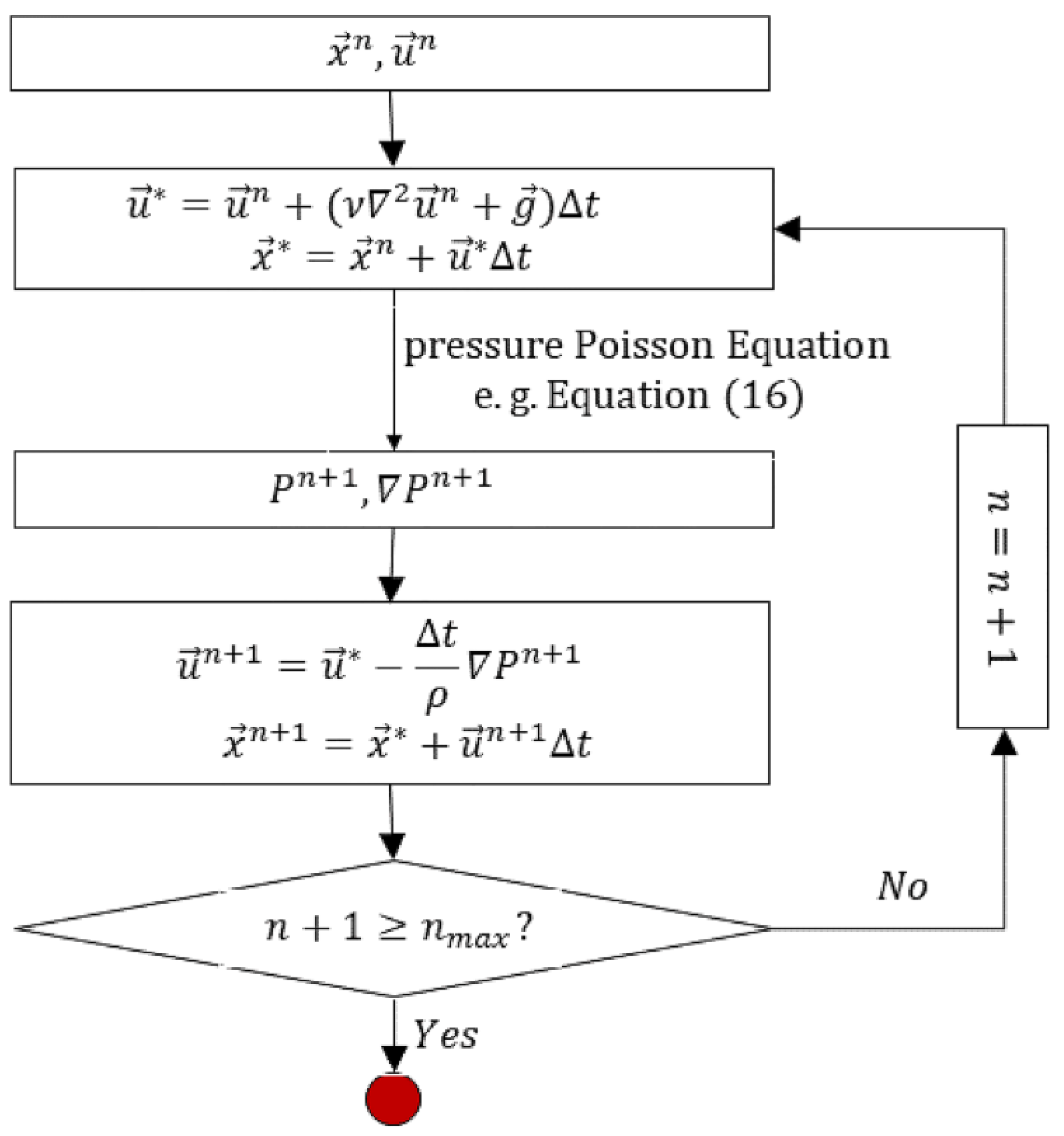
2. Original MPS Method

The original MPS method introduced in this section is based on Koshizuka et al. [1].

2.1. Governing Equations

The governing equations of the MPS method include the momentum equation (Equation (1)) and the mass conservation equation (Equation (2)):

$$\frac{d\overrightarrow{u}}{dt}=-\frac{1}{\rho }\nabla P+\nu {\nabla }^2\overrightarrow{u}+\overrightarrow{g}$$

(1)

$$\frac{d\rho }{dt}+\rho \nabla \cdot \overrightarrow{u}=0$$

(2)

where $\overrightarrow{u}$, $t$, $\rho$, $P$, $\nu$, and $\overrightarrow{g}$ represent velocity vector, time, density, pressure, viscous coefficient, and acceleration of gravity, respectively.

2.2. Gradient Operator and Laplacian Operator

The original MPS gradient operator can be represented as follows:

$${\langle \nabla f\rangle }_i=\frac{d}{n_0}{\displaystyle \sum _{j\ne i}\frac{f_j-f_i}{r_{ij}^2}{\overrightarrow{r}}_{ij}{w}_{ij}}$$

(3)

where $f$ denotes the physical quantity, $d$ represents the dimension of calculation, $n_0$ denotes the initial particle number density, ${\overrightarrow{r}}_{ij}$ represents the displacement vector from particle $i$ to particle $j$, and $w_{ij}$ represents the kernel function. In the original MPS method, $w_{ij}$ follows the equation

$$w_{ij}=\{\begin{array}{cc}\frac{r_e}{r_{ij}}-1,& r\le r_e;\\ 0,& \mathrm{others}.\end{array}$$

(4)

where $r_e$ represents the searching radius. Usually, $r_e=2.1l_0$, where $l_0$ denotes the particle resolution. The particle number density follows the equation

$$n(i)={\displaystyle \sum _{j\ne i}{w}_{ij}}$$

(5)

In order to prevent particle aggregation, the following pressure gradient equation (Equation (6)) is usually used:

$${\langle \nabla P\rangle }_i=\frac{d}{n_0}{\displaystyle \sum _{j\ne i}\frac{P_j-{\widehat{P}}_i}{r_{ij}^2}{\overrightarrow{r}}_{ij}{w}_{ij}}$$

(6)

where ${\widehat{P}}_i$ is the minimum pressure in the searching domain of particle $i$.

The original Laplacian operator follows the equation

$${\langle {\nabla }^{2}f\rangle }_i=\frac{2d}{\lambda n_0}{\displaystyle \sum _{j\ne i}\left(f_j-f_i\right)w_{ij}}$$

(7)

$$\lambda =\frac{{\displaystyle \sum _{j\ne i}{r}_{ij}{}^2{w}_{ij}}}{{\displaystyle \sum _{j\ne i}{w}_{ij}}}$$

(8)

2.3. Simulation Process of Traditional MPS Scheme

The MPS method is an operator-splitting scheme. Normally, it consists of an explicit step and an implicit correction step at each time step.

In the explicit step, an intermediate velocity ${\overrightarrow{u}}^{*}$ can be obtained using Equation (9):

$$\frac{{\overrightarrow{u}}^{*}-{\overrightarrow{u}}^n}{\Delta t}=\nu {\nabla }^2{\overrightarrow{u}}^n+\overrightarrow{g}$$

(9)

Then, in the implicit step, the velocity of the ${(n+1)}^{th}$ time step ${\overrightarrow{u}}^{n+1}$ can be calculated using Equation (10):

$$\frac{{\overrightarrow{u}}^{n+1}-{\overrightarrow{u}}^{*}}{\Delta t}=-\frac{1}{\rho }\nabla P^{n+1}$$

(10)

By combining Equations (9) and (10), the momentum equation is obtained. Taking the divergence of both sides of Equation (10), the following pressure Poisson equation is obtained:

$${\nabla }^2{P}^{n+1}=\frac{\rho }{\Delta t}\left(\nabla \cdot {\overrightarrow{u}}^{*}-\nabla \cdot {\overrightarrow{u}}^{n+1}\right)$$

(11)

For incompressible flows, ${\overrightarrow{u}}^{n+1}$ satisfies the following incompressible continuity equation:

$$\nabla \cdot {\overrightarrow{u}}^{n+1}=0$$

(12)

Substitute Equation (12) into Equation (11), and a DF-type (divergence-free type) pressure Poisson equation is obtained:

$${\nabla }^2{P}^{n+1}=\frac{\rho }{\Delta t}\nabla \cdot {\overrightarrow{u}}^{*}$$

(13)

From Equation (12) and Equation (2) (the mass conservation equation), the following equation can be obtained:

$$\frac{\rho -{\rho }^{*}}{\rho \Delta t}=\nabla \cdot {\overrightarrow{u}}^{*}$$

(14)

where ${\rho }^{*}$ denotes intermediate density.

By replacing $\rho$ and ${\rho }^{*}$ with $n_0$ and intermediate number density $n(i)$, respectively, on the left side of Equation (14), Equation (15) is obtained:

$$\frac{n(i)-n_0}{n_0\Delta t}=-\nabla \cdot {\overrightarrow{u}}^{*}$$

(15)

By combining Equations (13) and (15), a DI-type (density-invariant type) pressure Poisson equation is obtained (Equation (16)):

$${\nabla }^2{P}^{n+1}=-\frac{\rho }{\Delta t^2}\frac{n(i)-n_0}{n_0}$$

(16)

The simulation process of the original MPS scheme is shown in Figure 1. As is shown in the figure, the original MPS method directly solves the pressure Poisson equation to obtain the total pressure of fluid flow.

3. Proposed MPS Method

In this section, we present the details of the proposed MPS method. In Section 3.1, the hybrid DI/DF source term introduced for the proposed MPS method is presented. Then, a modified MPS scheme with a split-pressure Poisson equation is developed in Section 3.2. In Section 3.3, the consistent Laplacian operator proposed by Zhang et al. [15] is introduced. The new virtual particle technology is described in Section 3.4. Finally, the free surface judgment technique developed by Pan et al. [39] is presented in Section 3.5.

3.1. Improved Source Term of Pressure Poisson Equation

The pure DI-type source term of the pressure Poisson equation given by Equation (16) can ensure a stable particle number density, but the pressure oscillation can be exaggerated. In contrast, the pure DF-type source term given on the right-hand side of Equation (13) has better pressure behavior, but errors may accumulate regarding the particle number density. In order to combine the advantages of the two source terms, the following hybrid DI/DF term developed by Tanaka and Masunaga [32] is adopted in the proposed MPS method:

$${\nabla }^{2}P=\rho \left[\left(1-\gamma \right)\frac{\nabla \cdot {\overrightarrow{u}}^{*}}{\Delta t}-\gamma \frac{n(i)-n_0}{n_0\Delta t^2}\right]$$

(17)

where $\gamma$ is an empirical parameter. Generally, $\gamma =0.01$ is recommended.

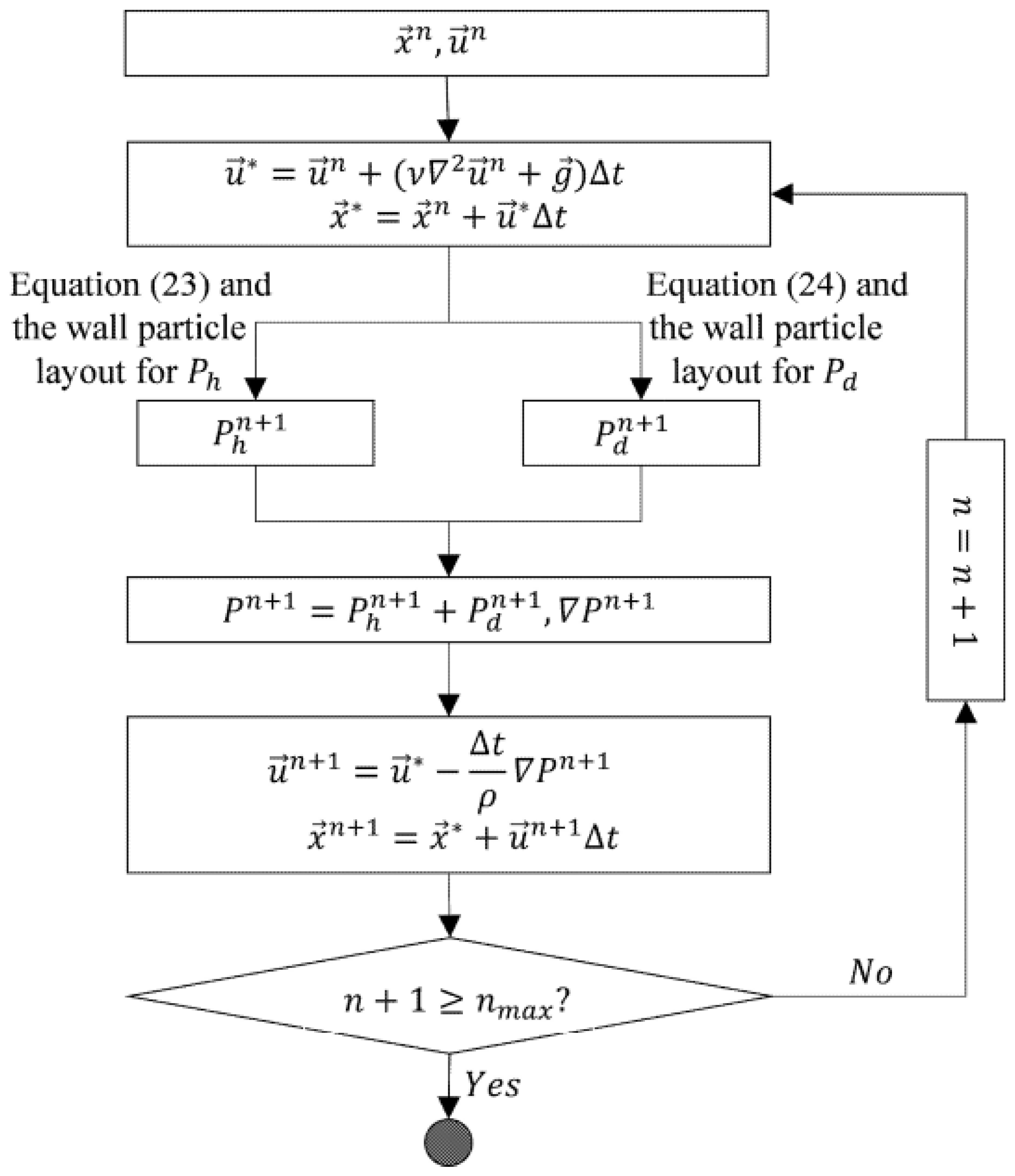
3.2. Modified MPS Scheme with a Split-Pressure Poisson Equation

In traditional MPS calculations, hydrostatic pressure cannot be reproduced stably and precisely because the Neumann boundary condition is not satisfied on the wall. One solution is to directly apply the Neumann boundary condition shown in Equation (18) to the wall boundary, as has been proposed by Lee et al. [29], Sun et al. [30], Tamai and Koshizuka [18], and Zhang et al. [38]. Here, we develop a modified MPS scheme in which the pressure Poisson equation is split into a hydrostatic pressure Laplacian equation and a dynamic pressure Poisson equation as another solution.

$${\frac{\partial P}{\partial n}|}_{{\Gamma }_N}=\left(\rho \overrightarrow{g}-{\frac{d\overrightarrow{u}}{dt}|}_{{\Gamma }_N}\right)\cdot \overrightarrow{n}$$

(18)

In the proposed MPS scheme, the total pressure $P$ is spit into the hydrostatic pressure $P_h$ and the dynamic pressure $P_d$.

$$P=P_h+P_d$$

(19)

By substituting Equation (19) into the pressure Poisson equation shown in Equation (17), we get the following:

$${\nabla }^2\left(P_h+P_d\right)=\rho \left[\left(1-\gamma \right)\frac{\nabla \cdot {\overrightarrow{u}}^{*}}{\Delta t}-\gamma \frac{n(i)-n_0}{n_0\Delta t^2}\right]$$

(20)

When we split the above equation into a Laplacian equation and a dynamic pressure Poisson equation, we get the following:

$${\nabla }^2{P}_h=0$$

(21)

$${\nabla }^2{P}_d=\rho \left[\left(1-\gamma \right)\frac{\nabla \cdot {\overrightarrow{u}}^{*}}{\Delta t}-\gamma \frac{n(i)-n_0}{n_0\Delta t^2}\right]$$

(22)

Regarding the Dirichlet condition and the wall boundary condition, $P_h$ and $P_d$ satisfy Equations (23) and (24), respectively:

$$\{\begin{array}{cc}{\nabla }^2{P}_h=0{,}_{}\hfill & \hfill {\mathrm{inner}}_{}{\mathrm{fluid}}_{}\mathrm{particle};\\ {\frac{\partial P_h}{\partial n}|}_{{\Gamma }_N}=\rho \overrightarrow{g}\cdot \overrightarrow{n},\hfill & \hfill {\mathrm{wall}}_{}{\mathrm{pressure}}_{}\mathrm{particle};\\ {P_h|}_{{\Gamma }_D}=0{,}_{}\hfill & \hfill {\mathrm{Dirichlet}}_{}\mathrm{particle}.\end{array}$$

(23)

$$\{\begin{array}{cc}{\nabla }^2{P}_d=\rho \left[\left(1-\gamma \right)\frac{\nabla \cdot {\overrightarrow{u}}^{*}}{\Delta t}-\gamma \frac{n(i)-n_0}{n_0\Delta t^2}\right],\hfill & \hfill {\mathrm{inner}}_{}\mathrm{particle};\hfill \\ {P_d|}_{{\Gamma }_D}=0{,}_{}\hfill & \hfill {\mathrm{Dirichlet}}_{}\mathrm{particle}.\hfill \end{array}$$

(24)

In Equation (24), “inner particle” refers to an arbitrary pressure particle (whether it is a fluid particle or a wall pressure particle) that is not judged to be a Dirichlet particle.

Two different wall particle layouts are used to calculate the hydrostatic pressure and dynamic pressure, respectively. The three-layer particle layout shown in Figure 2a is adopted to calculate the dynamic pressure $P_d$. This layout is identical to that of the original MPS method. In this layout, wall pressure particles are settled in the first layer and ghost particles are settled in the other layers in order to ensure accurate particle number density near the wall. The other three-layer particle layout, shown in Figure 2b, is adopted to calculate the hydrodynamic pressure $P_h$. In Figure 2b, two pressure particle layers and a ghost particle layer are involved. The particles in the first layer are treated as adhesion fluid particles. Therefore, they satisfy the Laplacian equation. The particles in the second layer, meanwhile, are wall boundary particles, which satisfy the wall boundary condition in Equation (23).

In Figure 2, particle layouts for a regular wall are presented. However, it is often necessary in practice to calculate cases with an irregular wall. For fixed walls with complex shapes, it may be difficult to directly deploy three-layer particle layouts. In this paper, we introduce an artificial bottom for use when calculating cases with irregular walls. As is shown in Figure 3, after the artificial bottom is introduced, the irregular computational domain becomes regular. Therefore, the three-layer particle layouts shown in Figure 2 can easily be deployed.

As the total pressure is split, the proposed MPS scheme is named an MPS scheme with a split-pressure Poisson equation (MPS-SP scheme). The simulation process of the MPS-SP scheme is presented in Figure 4. By comparing Figure 4 and Figure 1, it can be seen that the original MPS scheme directly calculates the total pressure $P$, while the MPS-SP scheme uses two different pressure equations to calculate the dynamic pressure $P_d$ and hydrostatic pressure $P_h$ and then obtains the total pressure $P$ by adding $P_d$ and $P_h$ together. We can also see from Figure 4 that different wall particle layouts are required to calculate the hydrostatic pressure and dynamic pressure in the MPS-SP scheme.

3.3. Laplacian Operator

The original Laplacian operator shown in Equation (7) has the property of physical conservation. However, it is inconsistent with the original gradient operator. In order to ensure physical conservation and consistency, we introduce the following Laplacian operator proposed by Zhang et al. [15]:

$${\nabla }^{2}f=\frac{2d}{n_0}{\displaystyle \sum _{j\ne i}\frac{f_j-f_i}{r_{ij}^2}{w}_{ij}}$$

(25)

The operator given by Equation (25) is physically conservative. According to [15], the Laplacian operator is derived by taking the divergence of the original gradient operator given by Equation (3). Therefore, it is consistent with the original gradient operator.

3.4. Improved Virtual Particle Technology with Given Position

In traditional MPS methods, free surface particles are generally regarded as the Dirichlet boundary, and the pressure of free surface particles is set to the same value (usually 0 Pa). According to the gradient operator shown in Equation (3), the interaction force between particle $i$ and particle $j$ can be expressed as follows:

$${\langle \nabla P\rangle }_{ij}=\frac{d}{n_0}\frac{P_j-P_i}{r_{ij}^2}{\overrightarrow{r}}_{ij}{w}_{ij}$$

(26)

If $i$ and $j$ are both free surface particles, then

$$\begin{array}{cc}{P}_j=P_i,& i,j\in {\mathrm{free}}_{}\mathrm{surface}\end{array}$$

(27)

Substituting Equation (27) into Equation (26) gives

$$\begin{array}{cc}{\langle \nabla P\rangle }_{ij}\equiv 0,& i,j\in {\mathrm{free}}_{}\mathrm{surface}\end{array}$$

(28)

Equation (28) indicates that there is zero interactive repulsive force between free surface particles, no matter how close they are. This may lead to particle overlapping and particle thrust on the free surface, finally causing numerical instability. The virtual particle techniques proposed by Chen et al. [35] and Shibata et al. [6] solve the problem of zero interaction force between free surface particles; however, these techniques are limited to the original Laplacian operator and its derivatives because the positions of virtual particles cannot be given. In this section, we develop an improved virtual particle technique with a given position that can be applied to an arbitrary Laplacian operator.

3.4.1. Classification of Free Surface Particles

Free surface particles are classified into splash particles and ordinary free surface particles. Splash particles are free surface particles without neighbors. Ordinary free surface particles are free surface particles with neighbors. Neighboring virtual particles are present only for ordinary free surface particles. Because splash particles are surrounded by a void, they are set as the Dirtichlet boundary, and their values of pressure are set to 0 Pa.

3.4.2. Position of a Virtual Particle

If $i$ is an ordinary free surface particle, then a neighboring virtual particle is present for $i$. The weight of the virtual particle $w_v$ is set to

$$w_v=n_0-n(i)$$

(29)

In addition, the intermediate velocity of the virtual particle ${\overrightarrow{u}}_v{}^{*}$ is set to

$${\overrightarrow{u}}_v^{*}={\overrightarrow{u}}_i^{*}$$

(30)

In general, particle distribution at the free surface is asymmetric. In this case, the following symmetry condition cannot be satisfied:

$${\displaystyle \sum _{\begin{array}{c}j\ne i\\ r_{ij}<r_e\end{array}}\frac{{\overrightarrow{r}}_{ij}}{r_{ij}^2}=0}$$

(31)

We assume the symmetry condition can be satisfied after the neighboring virtual particle is placed in ${\overrightarrow{r}}_{iv}$:

$$\frac{{\overrightarrow{r}}_{iv}}{r_{iv}^2}+{\displaystyle \sum _{\begin{array}{c}j\ne i\\ r_{ij}<r_e\end{array}}\frac{{\overrightarrow{r}}_{ij}}{r_{ij}^2}=0}$$

(32)

Therefore, the position of the virtual particle can be calculated according to the following equation:

$$\frac{{\overrightarrow{r}}_{iv}}{r_{iv}^2}={\displaystyle \sum _{\begin{array}{c}j\ne i\\ r_{ij}<r_e\end{array}}\frac{-{\overrightarrow{r}}_{ij}}{r_{ij}^2}}$$

(33)

Because the position of the virtual particle is known, the technique can be applied to arbitrary Laplacian operators.

3.4.3. Discrete Dynamic Pressure Poisson Equation on a Free Surface

In this study, the virtual particle technique is only applied to the dynamic pressure Poisson equation.

For inner particles, we combine Equations (25) and (24) to obtain the following discrete dynamic pressure Poisson equation:

$$\frac{2d}{n_0}{\displaystyle \sum _{j\ne i}\frac{P_{dj}-P_{di}}{r_{ij}^2}{w}_{ij}}=\rho \left[\left(1-\gamma \right)\frac{\nabla \cdot {\overrightarrow{u}}^{*}}{\Delta t}-\gamma \frac{n(i)-n_0}{n_0\Delta t^2}\right]$$

(34)

For ordinary free surface particles, after a neighboring virtual particle is introduced, the discrete slamming pressure Poisson equation can be expressed as follows:

$$\frac{2d}{n_0}{\displaystyle \sum _{j\ne i}\frac{P_{dj}-P_{di}}{r_{ij}^2}{w}_{ij}}+\frac{2d}{n_0}\frac{P_v-P_{di}}{r_{iv}^2}{w}_v=\rho \left[\left(1-\gamma \right)\frac{\nabla \cdot {\overrightarrow{u}}^{*}}{\Delta t}-\gamma \frac{n(i)+w_v-n_0}{n_0\Delta t^2}\right]$$

(35)

where $P_v$ refers to the pressure of the virtual particle. Usually, $P_v=0$.

Taking molds on both sides of Equation (33) gives

$$\frac{r_{iv}}{r_{iv}^2}=\left|{\displaystyle \sum _{j\ne i}\frac{-{\overrightarrow{r}}_{ij}}{r_{ij}^2}}\right|$$

(36)

Hence,

$$\frac{1}{r_{iv}^2}={\left|{\displaystyle \sum _{j\ne i}\frac{-{\overrightarrow{r}}_{ij}}{r_{ij}^2}}\right|}^2$$

(37)

By substituting Equations (29) and (37) into Equation (35), the discrete dynamic pressure Poisson equation of ordinary free surface particles can be obtained:

$$\frac{2d}{n_0}{\displaystyle \sum _{j\ne i}\frac{P_{dj}-P_{di}}{r_{ij}^2}{w}_{ij}}+\frac{2d}{n_0}\left(P_v-P_{di}\right){\left|{\displaystyle \sum _{j\ne i}\frac{-{\overrightarrow{r}}_{ij}}{r_{ij}^2}}\right|}^2\left(n_0-n(i)\right)=\rho \left(1-\gamma \right)\frac{\nabla \cdot {\overrightarrow{u}}^{*}}{\Delta t}$$

(38)

3.4.4. Pressure Gradient on a Free Surface

According to Equation (6), the pressure gradient of an ordinary free surface particle with a neighboring virtual particle can be expressed as follows:

$$\nabla P=\frac{2d}{n_0}\frac{P_v-{\widehat{P}}_i}{r_{iv}^2}{\overrightarrow{r}}_{iv}{w}_v+\frac{2d}{n_0}{\displaystyle \sum _{j\ne i}\frac{P_j-{\widehat{P}}_i}{r_{ij}^2}{\overrightarrow{r}}_{ij}{w}_{ij}}$$

(39)

On the free surface, the minimum pressure ${\widehat{P}}_i$ is equal to 0. At the same time, $P_v$ is equal to 0 as well. Therefore, the above equation can be expressed as follows:

$$\nabla P=\frac{2d}{n_0}{\displaystyle \sum _{j\ne i}\frac{P_j}{r_{ij}^2}{\overrightarrow{r}}_{ij}{w}_{ij}}$$

(40)

3.5. Judgement of Free Surface Particles

The original method proposed by Koshizuka et al. [1] judged free surface particles only by number density. It is thus a one-judgment method. Tanaka and Masunaga [32] proposed another one-judgment method that makes judgements based on the number of neighboring particles. These one-judgment methods are very simple, but they can easily cause misjudgments. Once an internal particle is misjudged as a free surface particle, the pressure field is distorted. In order to further reduce misjudgments, hybrid strategies have been developed, such as the two-judgment methods proposed by Lee et al. [29], Pan et al. [39], and Wan and Zhang [40]. There are also methods for judging the free surface particles using the geometric arrangement of neighboring particles, such as those proposed by Sun et al. [30], Shibata et al. [6], and Sun et al. [41].

In this paper, the two-judgment algorithm proposed by Pan et al. [39] is introduced to detect free surface particles.

If the following condition is satisfied, then particle $i$ is recognized as an inner particle:

$$\frac{n(i)}{n_0}\ge {\beta }_1$$

(41)

However, if Equation (42) is satisfied, particle $i$ is recognized as a free surface particle:

$$\frac{n(i)}{n_0}\le {\beta }_2$$

(42)

When Equation (43) is satisfied, a secondary judgement is required to further distinguish whether particle $i$ is a free surface particle.

$${\beta }_2\le \frac{n(i)}{n_0}\le {\beta }_1$$

(43)

In Equations (41)–(43), ${\beta }_1$ and ${\beta }_2$ are user-defined tuning parameters. In this paper, we chose ${\beta }_1=0.98$ and ${\beta }_2=0.85$.

For a particle that requires a secondary judgement, its neighboring region between $1.0l_0$ and $2.1l_0$ is divided into eight parts (as Figure 5 shows). If there are no neighboring particles in the two adjacent parts, then the particle is recognized as a free surface particle.

4. Verification

In the part of the study described in this section, several free surface flows were adopted to verify the proposed MPS method, including two hydrostatic problems, a dam-breaking problem, and a violent sloshing problem. First, the hydrostatic problems were used to verify the proposed method’s ability to reproduce the hydrostatic pressure. One hydrostatic problem involved a regular tank, and the other involved a tank with an irregular bottom. Then, the dam-breaking problem was adopted to verify the proposed method’s ability to calculate the slamming pressure on a solid wall. Finally, the violent sloshing problem was used to demonstrate the proposed method’s ability to simulate slamming pressure on a moving wall.

Table 1. Models for verification.

Model	MPS Scheme	Laplacian Operator	Virtual Particle Technique
MPS-OL	Original scheme	Original (Equation (7))	×
MPS-CL	Original scheme	Consistent (Equation (25))	×
MPS-CL-V	Original scheme	Consistent (Equation (25))	√, Equations (38) and (40)
MPS-SP-CL-V	MPS-SP scheme	Consistent (Equation (25))	√, Equations (38) and (40)

presents a brief description of the four computational models used in the verification analysis. In the MPS-OL model, the original MPS scheme and operators were used. In the MPS-CL model, the original MPS scheme was adopted, but the original Laplacian operator was substituted for the consistent operator proposed by Zhang et al. [15]. The MPS-CL-V model added the proposed virtual particle technique to the MPS-CL model. The MPS-SP-CL-V model adopted the MPS-SP scheme, the consistent Laplacian operator, and the proposed virtual particle technique. The free surface particle detection algorithm proposed by Pan et al. [39] and the improved source term (Equation (17)) proposed by Tanaka and Masunaga [32] were adopted in all the models listed in Table 1.

4.1. Hydrostatic Problems

The theoretical calculation of the hydrostatic pressure is possible. Through the simulation of hydrostatic problems, the ability of numerical methods to reproduce hydrostatic pressure can be compared. In the investigation described in this section, two hydrostatic cases were considered. One was in a regular rectangular tank, and the other was in a tank with an irregular bottom.

4.1.1. Hydrostatic Problem in a Regular Tank

Figure 6 shows the simulation domain of the hydrostatic problem in a regular tank. It was a $600 \mathrm{mm}$ long rectangular tank with a water depth of $500 \mathrm{mm}$. The spatial resolution $l_0=0.010\mathrm{m}$, and the time step length $∆t=0.0001\mathrm{s}$. The monitoring point A was set to observe the pressure variation. As is shown in Figure 6, point A was located at the middle of the bottom of the tank.

Figure 7 shows the fluid behavior of hydrostatic simulation using different models at t=3.0 s. It is clear from the results of the MPS-OL and MPS-CL that the particles on the free surface were slightly collapsed, and the particle distributions near the free surface became irregular. The particle distribution of the MPS-CL-V on the free surface was more regular than those of the MPS-OL and MPS-CL, but the free surface was still slightly collapsed. In contrast, the result of the MPS-SP-CL-V was the best. Not only was the free surface smooth, but the particles on the free surface were also evenly distributed.

Figure 8 shows the time histories of the hydrostatic pressure on point A. The pressure curves of MPS-OL, MPS-CL, and MPS-CL-V oscillated strongly at the initial stage, and then the amplitude gradually decreased with increasing in time. After about 1.4 s, the pressure results of the three methods tended to be stable. By comparing the amplitude of the three curves at the initial stage, it can be seen that MPS-OL > MPS-CL > MPS-CL-V. The adoption of the consistent Laplacian operator and the proposed virtual particle technique had a certain effect on alleviating the pressure oscillation, but it could not completely eliminate the long-period oscillation at the initial stage. In contrast, the MPS-SP-CL-V curve was not only stable after 1.4 s, but was also very stable at the initial stage. In addition, it can also be seen that the steady-state pressures of these four models were very close to that of the analytical solution. The steady-state pressure of MPS-SP-CL-V was slightly higher than that of the analytical solution, while those of the other curves were slightly lower than the analytical solution.

Table 2. Average error on point A between 2 and 3 s.

Model	MPS-OL	MPS-CL	MPS-CL-V	MPS-SP-CL-V
Average error	4.14%	3.27%	4.81%	2.89%

lists the average error on point A between 2 and 3 s for the four models. It is clear that the error of MPS-SP-CL-V was minimal. In general, MPS-SP-CL-V was able to reproduce hydrostatic pressure accurately and stably.

Table 3. Time cost of calculating 10,000 time steps using different models.

Model	MPS-OL	MPS-CL	MPS-CL-V	MPS-SP-CL-V
Time cost	20.3 min	20.3 min	22.2 min	87.6 min

lists the time cost of calculating 10,000 time steps using different models. The computer adopted in this study was equipped with an Intel Core i7-9700 3.0 GHz CPU with 32 GB of memory. A single core was used without any parallel computing. It is shown in Table 3 that the time cost of the MPS-SP-CL-V model was the highest. This is because the MPS-SP-CL-V model needed to solve both the pressure Laplacian equation and the pressure Poisson equation at each time step, while the other tree models only needed to calculate the pressure Poisson equation at each time step. It can also be seen that the time cost of the MPS-CL-V model was slightly greater than those of the MPS-OL model and the MPS-CL model. This is because the introduction of virtual particles onto the free surface increased the total number of calculated particles.

4.1.2. Hydrostatic Problem in a Tank with an Irregular Bottom

Figure 9 shows the simulation domain of the hydrostatic calculation in a tank with an irregular bottom. The width of the tank was 0.48 m, and the maximum fluid depth was 0.36 m. The particle spatial resolution $l_0=0.010\mathrm{m}$, and the time step length $∆t=0.0001\mathrm{s}$. The monitoring point S was set to observe the pressure variation. Point S was located at the middle of the bottom, and the depth was 0.26 m away from the free surface. As is shown in Figure 9, the irregular computational domain became regular after the artificial bottom was introduced.

Figure 10 shows the fluid behavior of the hydrostatic simulation in a tank with an irregular bottom using the MPS-SP-CL-V model at t = 3.0 s. It is clear from the figure that the free surface remained flat and the fluid particles in the tank maintained a regular distribution. The pressure distribution was also smooth. Figure 11 shows the time history of the hydrostatic pressure on point S. It is clear that the curve of the MPS-SP-CL-V model was almost consistent with that of the analytical solution. In general, both Figure 10 and Figure 11 indicate that the MPS-SP-CL-V model also reproduced the hydrostatic pressure well when simulating a case with an irregular bottom.

4.2. Dam-Breaking Experiment

The dam-breaking experiment conducted by Lobovský et al. [42] was simulated using the models shown in Table 1. The experiment was conducted in a glass tank with 0.600 m height and 1.610 m length (shown in Figure 12). The initial width and height of the water column were both 0.600 m. Two monitoring points, B1 and B2, were set to observe the pressure variation. As is shown in Figure 12, B1 was located in the left corner of the tank. The other monitoring point, B2, was located in the right corner. These two points were both 3 mm from the bottom. B1 was in the area where strong slamming would occur, while B2 was in the area farthest from the strong slamming area. The simulations were performed at spatial resolution $l_0=0.0050\mathrm{m}$ and time step length $∆t=0.0001\mathrm{s}$.

Figure 13 shows the particle distributions and the pressure contours of the dam-breaking fluid flows simulated by the four models. The nonsmooth free surface and unnatural pressure field were quite obvious in the pictures of the MPS-OL model, in which the original MPS scheme and the original Laplacian operator were used. The free surfaces in the pictures of the MPS-CL were smoother than those of the MPS-OL, but the pressure fields were still not smooth. The pictures of the MPS-CL-V showed a smoother free surface and pressure distribution; however, the pressure on the right-side wall was unstable over time. Compared to the results obtained by the other models, the pressure field and the free surface of the MPS-SP-CL-V were much better.

Figure 14a1–a4 presents the time histories of pressure acting on B1 calculated by the four models. The pressure fluctuation of the MPS-OL was frequent and significant. Compared to the MPS-OL, the pressure fluctuation of the MPS-CL was slightly mitigated. After applying the proposed virtual particle technique, the pressure curves of the MPS-CL-V and the MPS-SP-CL-V were much more stable than those of the MPS-CL. Figure 14b1–b4 presents the time histories of pressure acting on B2 calculated by the four models. As is shown in Figure 14b1,b2, long-term, large-amplitude pressure fluctuations and short-term, small-amplitude pressure fluctuations appeared on both the MPS-OL and MPS-CL curves. As the MPS-CL-V curve shows in Figure 14b3, the amplitude of short-period fluctuation was suppressed, but the amplitude of long-period fluctuation was still significant. Compared to the above three curves (Figure 14b1–b3), it is obvious that the results of the MPS-SP-CL-V shown in Figure 14b4 had the best pressure stability. In the figure, both the long-period and short-period fluctuation are alleviated significantly, which makes the curve of the MPS-SP-CL-V look much smoother than the others. In general, whether at point B1, close to the strong slamming area, or at point B2, far away from the strong slamming area, the time histories of the pressure calculated by MPS-SP-CL-V appeared to be very stable.

Figure 15 presents the pressure curves of point B1 calculated by MPS-SP-CL-V and the δ-SPH method. Both curves were calculated under a particle resolution of $l_0=0.005\mathrm{m}$. The numerical data of the δ-SPH method were extracted from You et al. [43]. As is shown in the figure, the peak values of the two curves (both about 3.5) were slightly higher than those from the experiment (about 3), and both curves were consistent with the experimental results of Lobovský et al. [42]. When comparing the two curves, it is obvious that the δ-SPH curve is smoother, while the result of the MPS-SP-CL-V was closer to the experiment data.

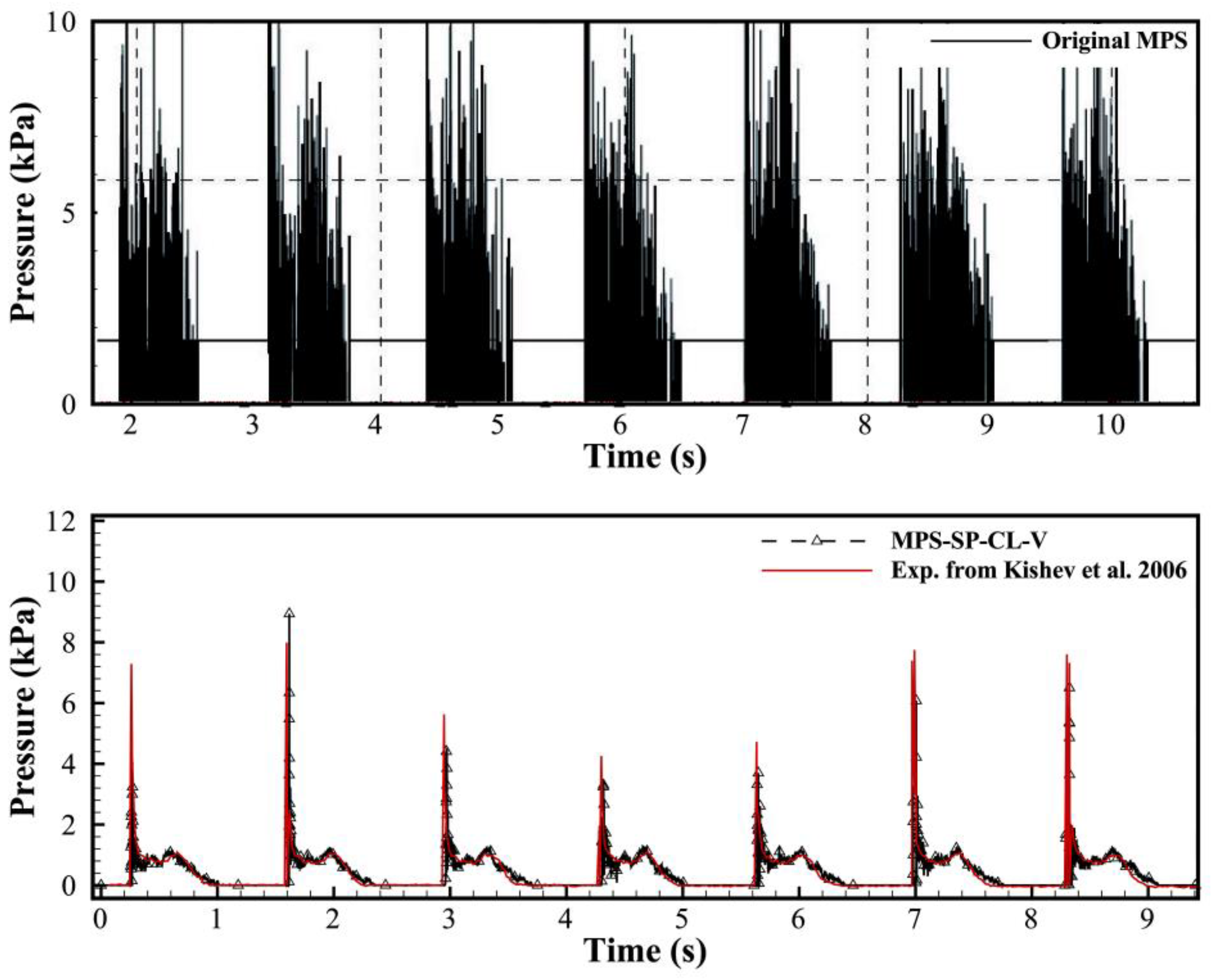
4.3. Violent Sloshing

As described in this section, a violent sloshing process in a rectangular tank was simulated using the proposed method. As Figure 16 shows, the tank was 600 mm wide and 300 mm high. The initial water depth of the tank was 120 mm. A monitoring point C to detect pressure variation was located on the right wall 100 mm from the bottom. The tank was oscillated in the horizontal direction, and the motion followed the below equation:

$$X=X_a\sin (\omega t)$$

(44)

where $X$ represents the horizontal displacement of the tank, $X_a$ refers to the amplitude of the oscillation, and $\omega$ denotes the circular frequency of the excitation. In this paper, $X_a=0.05\mathrm{m}$, and circular frequency $\omega =4.8332\mathrm{rad}\cdot {\mathrm{s}}^{-1}$(corresponding to the oscillation period $T=1.3\mathrm{s}$). The time step length of the simulation $\Delta t=0.0001\mathrm{s}$, and the spatial resolution $l_0=0.005\mathrm{m}$.

Figure 17 presents the free surface profiles of both the experimental results of Kishev et al. [44] and the MPS-SP-CL-V results at $0.1T$, $0.2T$, and $0.3T$, where $T$ is the oscillation period of the tank (1.3 s). The contour is the pressure distribution. As the figure shows, the pressure distribution distributed smoothly, and the free surface profiles of the MPS-SP-CL-V had good agreement with those of the experiment. Figure 18 shows the comparison of the pressure values from the original MPS method, the experiment of Kishev et al. [44], and the MPS-SP-CL-V method. From the figure, it is clear that the oscillation of pressure in the results of the original MPS method was huge and highly frequent. In contrast, the MPS-SP-CL-V method could successfully capture the typical pressure characteristics. It can also be seen from the figure that the pressure profile of the MPS-SP-CL-V was in good agreement with that of the experiment.

5. Conclusions

As a particle method based on a Lagrangian description, the MPS method can easily capture variations in an interface or free surface. It thus has natural advantages in dealing with free surface flow problems. However, in traditional MPS methods, hydrostatic pressure cannot be reproduced exactly and stably at every moment because the Neumann boundary condition is not satisfied on wall pressure particles. In addition, due to there being no interaction force between the free surface particles, particle thrust occurs on the free surface, which results in unphysical pressure oscillation. Although some virtual particle techniques have been developed to increase the interactions between particles on the free surface, these techniques do not give the positions of virtual particles, so they are limited to the original Laplacian operator and its derivatives. In order to remedy these problems, we propose a modified MPS method using the following techniques. First, a modified MPS scheme with a split-pressure Poisson equation is proposed to ensure the reproduction of the hydrostatic pressure. Then, we develop a new virtual particle technique in which the expression of the position of virtual particles is given. Therefore, the virtual particle technique can be extended to arbitrary Laplacian operators. In addition, a consistent Laplacian operator is introduced to replace the original Laplacian operator. In addition, a two-judgment technique and a hybrid DI/DF source term are adopted in the proposed MPS method.

Hydrostatic, dam-breaking, and sloshing examples were applied to verify these techniques. The original MPS method and the four models listed in Table 1 (including MPS-OL, MPS-CL, MPS-CL-V, and MPS-SP-CL-V) were involved in the verification. By discussing and comparing the simulation results of these methods, we drew the following conclusions:

• The stability of the consistent Laplacian operator was better than that of the original operator, but the degree of enhancement was limited;
• The proposed virtual particle technique applied to the consistent Laplacian operator was demonstrated to be effective for suppressing unphysical pressure fluctuation;
• Hydrostatic pressure can be reproduced stably and accurately by the MPS-SP-CL-V method in which the modified MPS scheme with a split-pressure Poisson equation is adopted;
• A remarkable enhancement in stability was demonstrated when using the MPS-SP-CL-V method to simulate the dam-breaking problem and the violent sloshing problem.

References

1. Koshizuka, S.; Tamako, H.; Oka, Y. A Particle Method for Incompressible Viscous Flow With Fluid Fragmentation. Comput. Fluid Dyn. J. 1995, 4, 29–46. [Google Scholar]
2. Huang, Y.; Zhu, C. Numerical Analysis of Tsunami–Structure Interaction Using a Modified MPS Method. Nat. Hazards 2015, 75, 2847–2862. [Google Scholar] [CrossRef]
3. Pan, X.J.; Zhang, H.X.; Lu, Y.T. Numerical Simulation of Viscous Liquid Sloshing by Moving-Particle Semi-Implicit Method. J. Mar. Sci. Appl. 2008, 7, 184–189. [Google Scholar] [CrossRef]
4. Pan, X.J.; Zhang, H.X.; Sun, X.Y. Numerical Simulation of Sloshing with Large Deforming Free Surface by MPS-LES Method. China Ocean Eng. 2012, 26, 653–668. [Google Scholar] [CrossRef]
5. Shibata, K.; Koshizuka, S.; Sakai, M.; Tanizawa, K. Lagrangian Simulations of Ship-Wave Interactions in Rough Seas. Ocean Eng. 2012, 42, 13–25. [Google Scholar] [CrossRef]
6. Shibata, K.; Masaie, I.; Kondo, M.; Murotani, K.; Koshizuka, S. Improved Pressure Calculation for the Moving Particle Semi-Implicit Method. Comput. Part. Mech. 2015, 2, 91–108. [Google Scholar] [CrossRef] [Green Version]
7. Shibata, K.; Koshizuka, S.; Sakai, M.; Tanizawa, K.; Ota, S. Numerical Analysis of Acceleration of a Free-Fall Lifeboat Using the MPS Method. Int. J. Offshore Polar Eng. 2013, 23, 279–285. [Google Scholar]
8. Sun, Z.; Chen, X.; Xi, G.; Liu, L.; Chen, X. Mass Transfer Mechanisms of Rotary Atomization: A Numerical Study Using the Moving Particle Semi-Implicit Method. Int. J. Heat Mass Transf. 2017, 105, 90–101. [Google Scholar] [CrossRef]
9. Yang, C.; Zhang, H. Numerical Simulation of the Interactions between Fluid and Structure in Application of the MPS Method Assisted with the Large Eddy Simulation Method. Ocean Eng. 2018, 155, 55–64. [Google Scholar] [CrossRef]
10. Duan, G.; Chen, B.; Zhang, X.; Wang, Y. A Multiphase MPS Solver for Modeling Multi-Fluid Interaction with Free Surface and Its Application in Oil Spill. Comput. Methods Appl. Mech. Eng. 2017, 320, 133–161. [Google Scholar] [CrossRef] [Green Version]
11. Chen, R.; Tian, W.; Su, G.H.; Qiu, S.; Ishiwatari, Y.; Oka, Y. Numerical Investigation on Bubble Dynamics during Flow Boiling Using Moving Particle Semi-Implicit Method. Nucl. Eng. Des. J. 2010, 240, 3830–3840. [Google Scholar] [CrossRef]
12. Chen, R.H.; Tian, W.X.; Su, G.H.; Qiu, S.Z.; Ishiwatari, Y.; Oka, Y. Numerical Investigation on Coalescence of Bubble Pairs Rising in a Stagnant Liquid. Chem. Eng. Sci. 2011, 66, 5055–5063. [Google Scholar] [CrossRef]
13. Koshizuka, S.; Oka, Y. Moving-Particle Semi-Implicit Method for Fragmentation of Incompressible Fluid. Nucl. Sci. Eng. 1996, 123, 421–434. [Google Scholar] [CrossRef]
14. Ng, K.C.; Hwang, Y.H.; Sheu, T.W.H. On the Accuracy Assessment of Laplacian Models in MPS. Comput. Phys. Commun. 2014, 185, 2412–2426. [Google Scholar] [CrossRef]
15. Zhang, S.; Morita, K.; Fukuda, K.; Shirakawa, N. An Improved MPS Method for Numerical Simulations of Convective Heat Transfer Problems. Int. J. Numer. Methods Fluids 2006, 51, 31–47. [Google Scholar] [CrossRef]
16. Khayyer, A.; Gotoh, H. A Higher Order Laplacian Model for Enhancement and Stabilization of Pressure Calculation by the MPS Method. Appl. Ocean Res. 2010, 32, 124–131. [Google Scholar] [CrossRef]
17. Xu, T.; Jin, Y.C. Improvements for Accuracy and Stability in a Weakly-Compressible Particle Method. Comput. Fluids 2016, 137, 1–14. [Google Scholar] [CrossRef]
18. Tamai, T.; Koshizuka, S. Least Squares Moving Particle Semi-Implicit Method. Comput. Part. Mech. 2014, 1, 277–305. [Google Scholar] [CrossRef] [Green Version]
19. Duan, G.; Yamaji, A.; Koshizuka, S.; Chen, B. The Truncation and Stabilization Error in Multiphase Moving Particle Semi-Implicit Method Based on Corrective Matrix: Which Is Dominant? Comput. Fluids 2019, 190, 254–273. [Google Scholar] [CrossRef]
20. Duan, G.; Yamaji, A.; Koshizuka, S. A Novel Multiphase MPS Algorithm for Modeling Crust Formation by Highly Viscous Fluid for Simulating Corium Spreading. Nucl. Eng. Des. 2019, 343, 218–231. [Google Scholar] [CrossRef]
21. Liu, X.; Morita, K.; Zhang, S. A Stable Moving Particle Semi-Implicit Method with Renormalized Laplacian Model Improved for Incompressible Free-Surface Flows. Comput. Methods Appl. Mech. Eng. 2019, 356, 199–219. [Google Scholar] [CrossRef]
22. Toyota, E. A Particle Method with Variable Spatial Resolution for Incompressible Flows. Proc. 19th Symp. Comput. Fluid Dyn. 2005, 2005, 10030478899. [Google Scholar]
23. Khayyer, A.; Gotoh, H. Modified Moving Particle Semi-Implicit Methods for the Prediction of 2D Wave Impact Pressure. Coast. Eng. 2009, 56, 419–440. [Google Scholar] [CrossRef]
24. Jandaghian, M.; Shakibaeinia, A. An Enhanced Weakly-Compressible MPS Method for Free-Surface Flows. Comput. Methods Appl. Mech. Eng. 2020, 360, 112771. [Google Scholar] [CrossRef]
25. Khayyer, A.; Gotoh, H. Enhancement of Stability and Accuracy of the Moving Particle Semi-Implicit Method. J. Comput. Phys. 2011, 230, 3093–3118. [Google Scholar] [CrossRef]
26. Wang, L.; Jiang, Q.; Zhang, C. Improvement of Moving Particle Semi-Implicit Method for Simulation of Progressive Water Waves. Int. J. Numer. Methods Fluids 2017, 85, 636–666. [Google Scholar] [CrossRef]
27. Liu, X.; Morita, K.; Zhang, S. An Advanced Moving Particle Semi-Implicit Method for Accurate and Stable Simulation of Incompressible Flows. Comput. Methods Appl. Mech. Eng. 2018, 339, 467–487. [Google Scholar] [CrossRef]
28. Khayyer, A.; Gotoh, H. A 3D Higher Order Laplacian Model for Enhancement and Stabilization of Pressure Calculation in 3D MPS-Based Simulations. Appl. Ocean Res. 2012, 37, 120–126. [Google Scholar] [CrossRef]
29. Lee, B.H.; Park, J.C.; Kim, M.H.; Hwang, S.C. Step-by-Step Improvement of MPS Method in Simulating Violent Free-Surface Motions and Impact-Loads. Comput. Methods Appl. Mech. Eng. 2011, 200, 1113–1125. [Google Scholar] [CrossRef]
30. Sun, Z.; Djidjeli, K.; Xing, J.T.; Cheng, F. Modified MPS Method for the 2D Fluid Structure Interaction Problem with Free Surface. Comput. Fluids 2015, 122, 47–65. [Google Scholar] [CrossRef] [Green Version]
31. Kondo, M.; Koshizuka, S. Improvement of Stability in Moving Particle Semi-Implicit Method. Int. J. Numer. Methods Fluids 2011, 65, 638–654. [Google Scholar] [CrossRef]
32. Tanaka, M.; Masunaga, T. Stabilization and Smoothing of Pressure in MPS Method by Quasi-Compressibility. J. Comput. Phys. 2010, 229, 4279–4290. [Google Scholar] [CrossRef]
33. Guo, K.; Chen, R.; Qiu, S.; Tian, W.; Su, G. An Improved Multiphase Moving Particle Semi-Implicit Method in Bubble Rising Simulations with Large Density Ratios. Nucl. Eng. Des. 2018, 340, 370–387. [Google Scholar] [CrossRef]
34. Li, D.; Zhang, H.; Yao, H. An Accurate and Stable Alternating Directional Moving Particle Semi-Implicit Method for Incompressible Flow Simulation. Adv. Mech. Eng. 2022, 14, 16878132221112570. [Google Scholar] [CrossRef]
35. Chen, X.; Xi, G.; Sun, Z.G. Improving Stability of MPS Method by a Computational Scheme Based on Conceptual Particles. Comput. Methods Appl. Mech. Eng. 2014, 278, 254–271. [Google Scholar] [CrossRef]
36. Guermond, J.L.; Minev, P.; Shen, J. An Overview of Projection Methods for Incompressible Flows. Comput. Methods Appl. Mech. Eng. 2006, 195, 6011–6045. [Google Scholar] [CrossRef] [Green Version]
37. Rannacher, R. On Chorin’s Projection Method for the Incompressible Navier-Stokes Equations. Navier-Stokes Equ. II Theory Numer. Methods 1992, 1530, 167–183. [Google Scholar] [CrossRef]
38. Zhang, G.; Wu, J.; Sun, Z.; el Moctar, O.; Zong, Z. Numerically Simulated Flooding of a Freely-Floating Two-Dimensional Damaged Ship Section Using an Improved MPS Method. Appl. Ocean Res. 2020, 101, 102207. [Google Scholar] [CrossRef]
39. Pan, X.J.; Zhang, H.X.; Sun, X.Y. A Free Surfacetraced Method for Moving Particle Semi-Implicit Method. Shanghai Jiaotong Daxue Xuebao J. Shanghai Jiaotong Univ. 2010, 44, 134–138. (In Chinese) [Google Scholar]
40. Zhang, Y.; Wang, D. Apply MPS Method to Simulate Liquid Sloshing in LNG Tang. In Proceedings of the Twenty-second International Offshore and Polar Engineering Conference, Rhodes, Greece, 17 June 2012; pp. 381–391. [Google Scholar]
41. Sun, C.; Shen, Z.; Zhang, M. Surface Treatment Technique of MPS Method for Free Surface Flows. Eng. Anal. Bound. Elem. 2019, 102, 60–72. [Google Scholar] [CrossRef]
42. Lobovský, L.; Botia-Vera, E.; Castellana, F.; Mas-Soler, J.; Souto-Iglesias, A. Experimental Investigation of Dynamic Pressure Loads during Dam Break. J. Fluids Struct. 2014, 48, 407–434. [Google Scholar] [CrossRef] [Green Version]
43. You, Y.; Khayyer, A.; Zheng, X.; Gotoh, H.; Ma, Q. Enhancement of δ-SPH for Ocean Engineering Applications through Incorporation of a Background Mesh Scheme. Appl. Ocean Res. 2021, 110, 102508. [Google Scholar] [CrossRef]
44. Kishev, Z.R.; Hu, C.; Kashiwagi, M. Numerical Simulation of Violent Sloshing by a CIP-Based Method. J. Mar. Sci. Technol. 2006, 11, 111–122. [Google Scholar] [CrossRef]
Figure 1. Simulation process of the original MPS scheme.
Jmse 11 00215 g001
Figure 2. Wall particle layouts for calculating the (a) dynamic pressure and (b) hydrostatic pressure.
Jmse 11 00215 g002
Figure 3. Diagrammatic sketch of the artificial bottom of an irregular wall. (a) The computational domain is irregular before the artificial bottom is introduced. (b) The irregular computational domain becomes regular after introducing the artificial bottom.
Jmse 11 00215 g003
Figure 4. Simulation process of the MPS-SP scheme.
Jmse 11 00215 g004
Figure 5. Schematic diagram of the secondary judgement.
Jmse 11 00215 g005
Figure 6. Simulation domain of the hydrostatic calculation in a regular tank.
Jmse 11 00215 g006
Figure 7. Fluid behavior of hydrostatic simulation in a regular tank using different models at t = 3.0 s.
Jmse 11 00215 g007
Figure 8. Time histories of the hydrostatic pressure on point A.
Jmse 11 00215 g008
Figure 9. Simulation domain of the hydrostatic calculation in a tank with an irregular bottom.
Jmse 11 00215 g009
Figure 10. Fluid behavior of hydrostatic simulation in a tank with an irregular bottom using the MPS-SP-CL-V model at t = 3.0 s.
Jmse 11 00215 g010
Figure 11. Time histories of the hydrostatic pressure on point S.
Jmse 11 00215 g011
Figure 12. Schematic diagram of pool size.
Jmse 11 00215 g012
Figure 13. Particle distributions and pressure contours of dam-breaking fluid flows at t = 316.7 ms, 413.4 ms, and 463.3 ms.
Jmse 11 00215 g013
Figure 14. Time histories of pressure acting on B1 and B2 calculated by the models. (a1) Pressure on B1 calculated by MPS-OL; (a2) Pressure on B1 calculated by MPS-CL; (a3) Pressure on B1 calculated by MPS-CL-V; (a4) Pressure on B1 calculated by MPS-SP-CL-V; (b1) Pressure on B2 calculated by MPS-OL; (b2) Pressure on B2 calculated by MPS-CL; (b3) Pressure on B2 calculated by MPS-CL-V; (b4) Pressure on B2 calculated by MPS-SP-CL-V. The experiment curve of the pressure on point B1 is from Lobovský et al. [42].
Jmse 11 00215 g014
Figure 15. Pressure curves of point B1 calculated by MPS-SP-CL-V and the δ-SPH method ( l 0 = 0.005   m ). The curves of the δ-SPH method and the experiment are from You et al. [43] and Lobovský et al. [42], respectively.
Jmse 11 00215 g015
Figure 16. Schematic diagram of the dimensions of the tank.
Jmse 11 00215 g016
Figure 17. Comparison of free surface profiles of the MPS-SP-CL-V with the experimental results of Kishev et al. [44].
Jmse 11 00215 g017
Figure 18. Comparison of the pressure in the experiment of Kishev et al. [44] and the original MPS method of Lee et al. [29].
Jmse 11 00215 g018