

An Improved Sea Spray-Induced Heat Flux Algorithm and Its Application in the Case Study of Typhoon Mangkhut (2018)

Abstract
:1. Introduction
2. Data and Model Descriptions
2.1. FASTEX Dataset
2.2. Model Description and Configuration
2.2.1. Atmospheric Model
2.2.2. Wave Model
3. An Improved Algorithm YJ22 and Its Application
3.1. The Process of Proposing AN15 and Its Problems
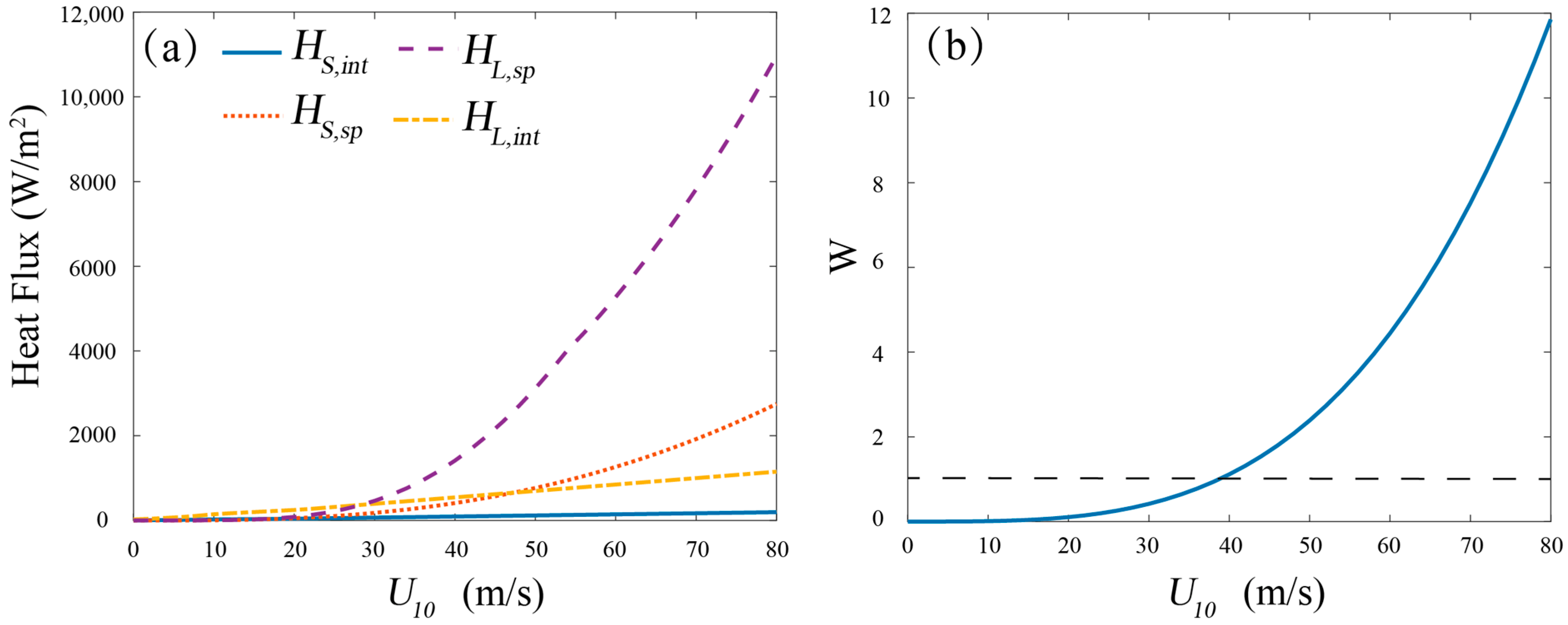
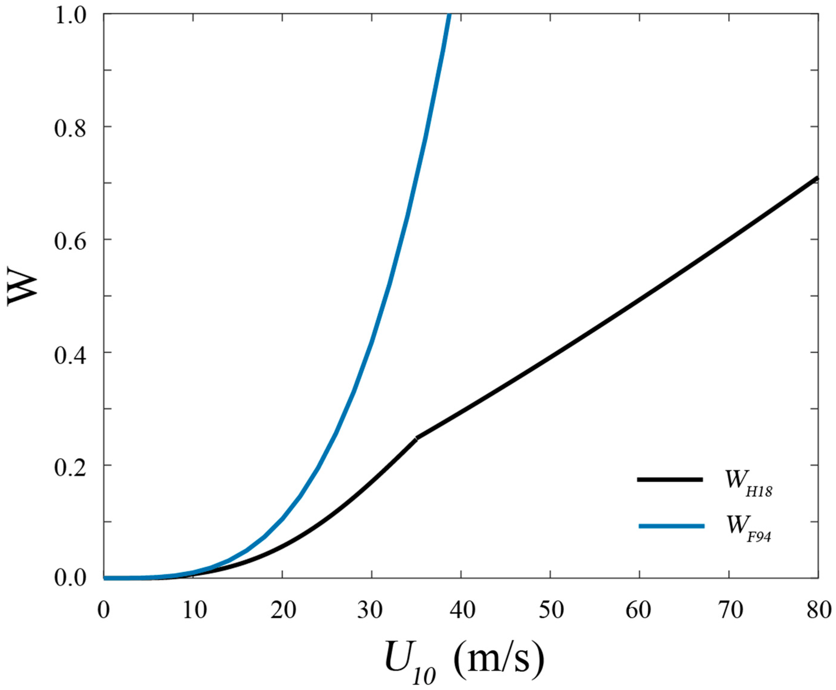
3.2. An Improved Sea Spray-Induced Heat Flux Algorithm YJ22
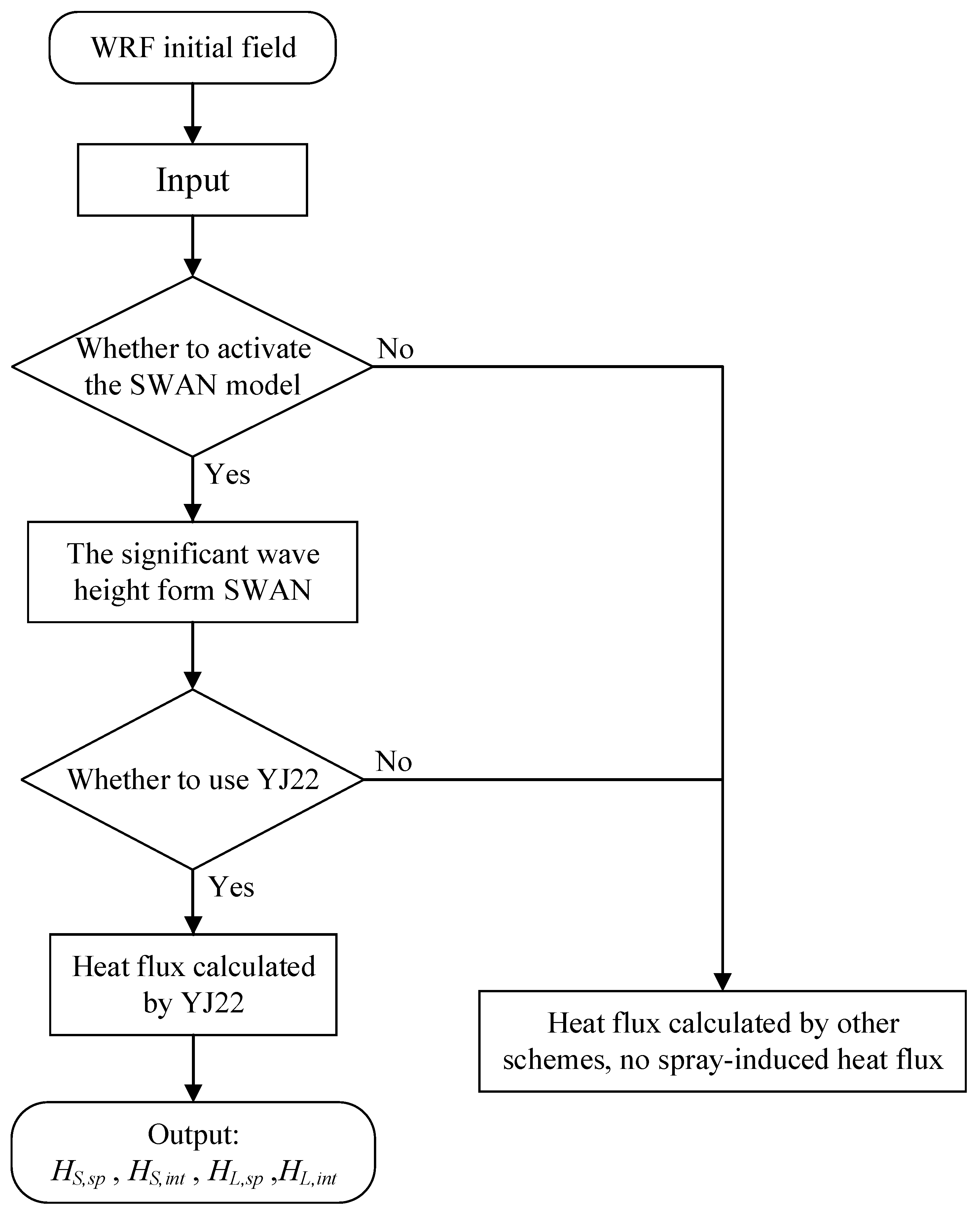
3.3. Application of the YJ22 in the COAWST Model
| Algorithm 1. The process of calculating the air–sea heat flux by the YJ22 algorithm. |
| Known: height , wind speed , air temperature , relative humidity , sea surface temperature SST, sea level pressure SLP, significant wave height , salinity S |
| Required: , , , |
| Step 1: ← FIND_USTAR() and ← NU |
| Step 2: ← MAIN_FLUX Step 3: ← SPRAY_FLUX |
4. Case Introduction and Experimental Design
4.1. An Overview of Super Typhoon Mangkhut
4.2. Experiments Design
5. Results and Discussion
5.1. Effect of Spray-Induced Heat Fluxes on TC Track and Intensity
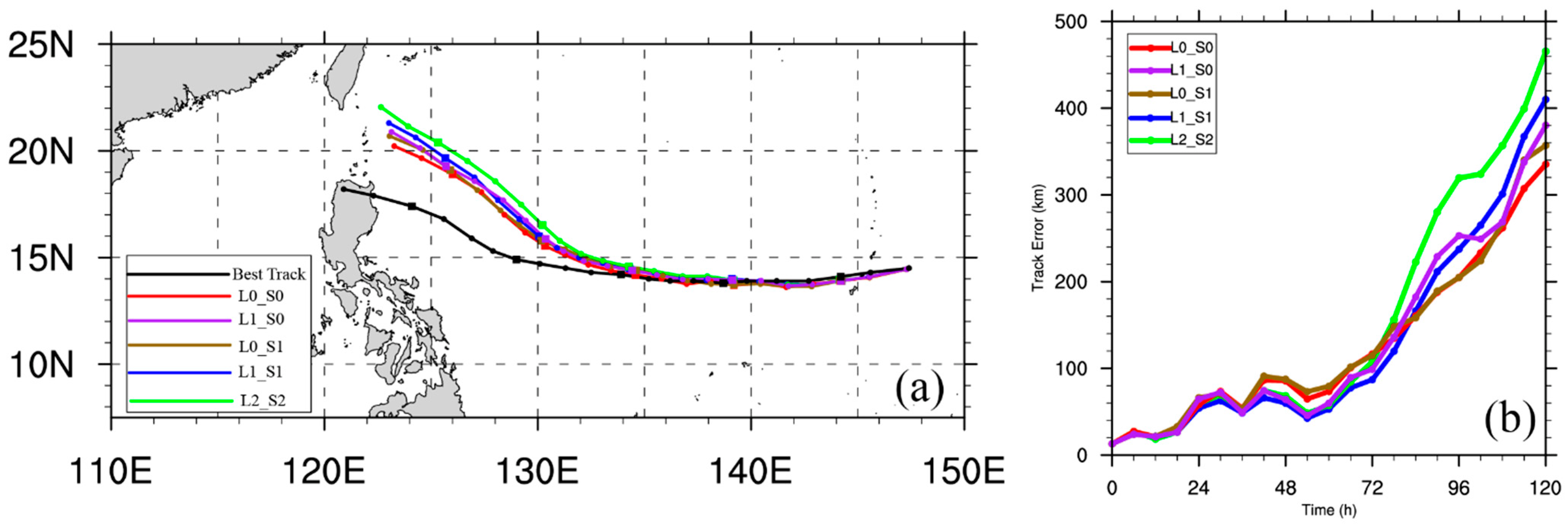
5.1.1. TC Track
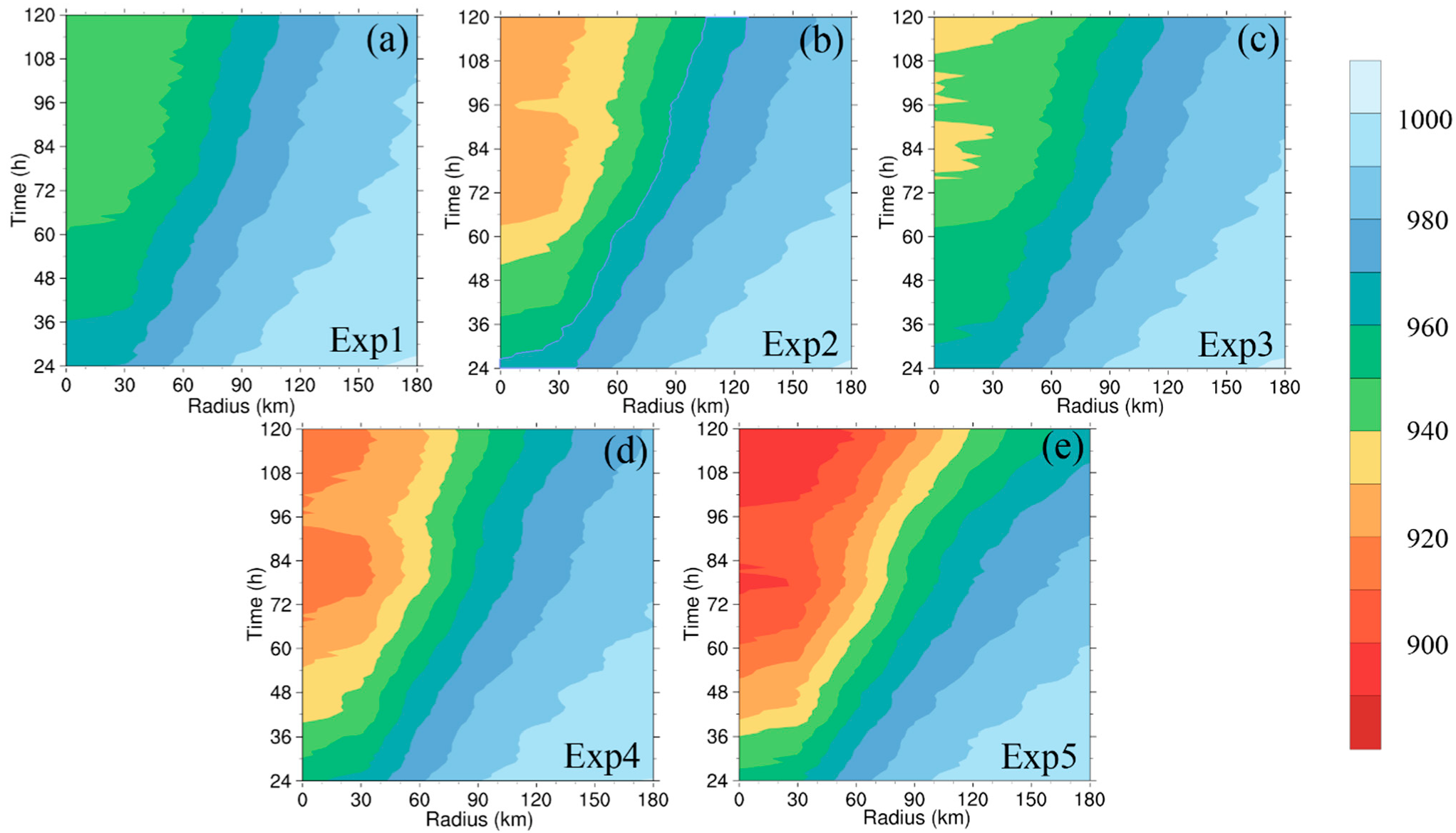
5.1.2. TC Intensity
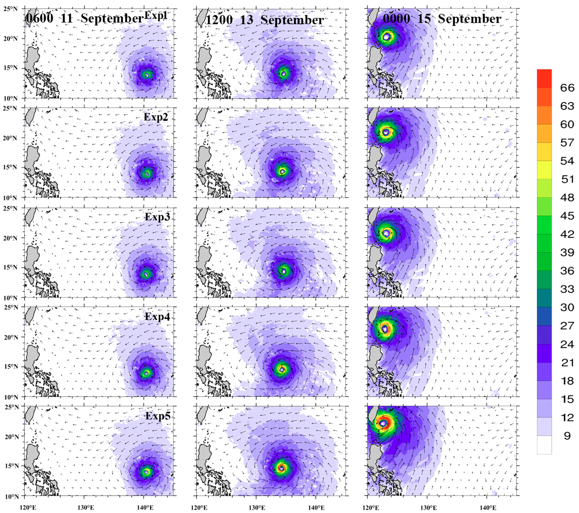
5.2. Effects of Sea Spray-Induced Heat Flux on the Evolution of TCs
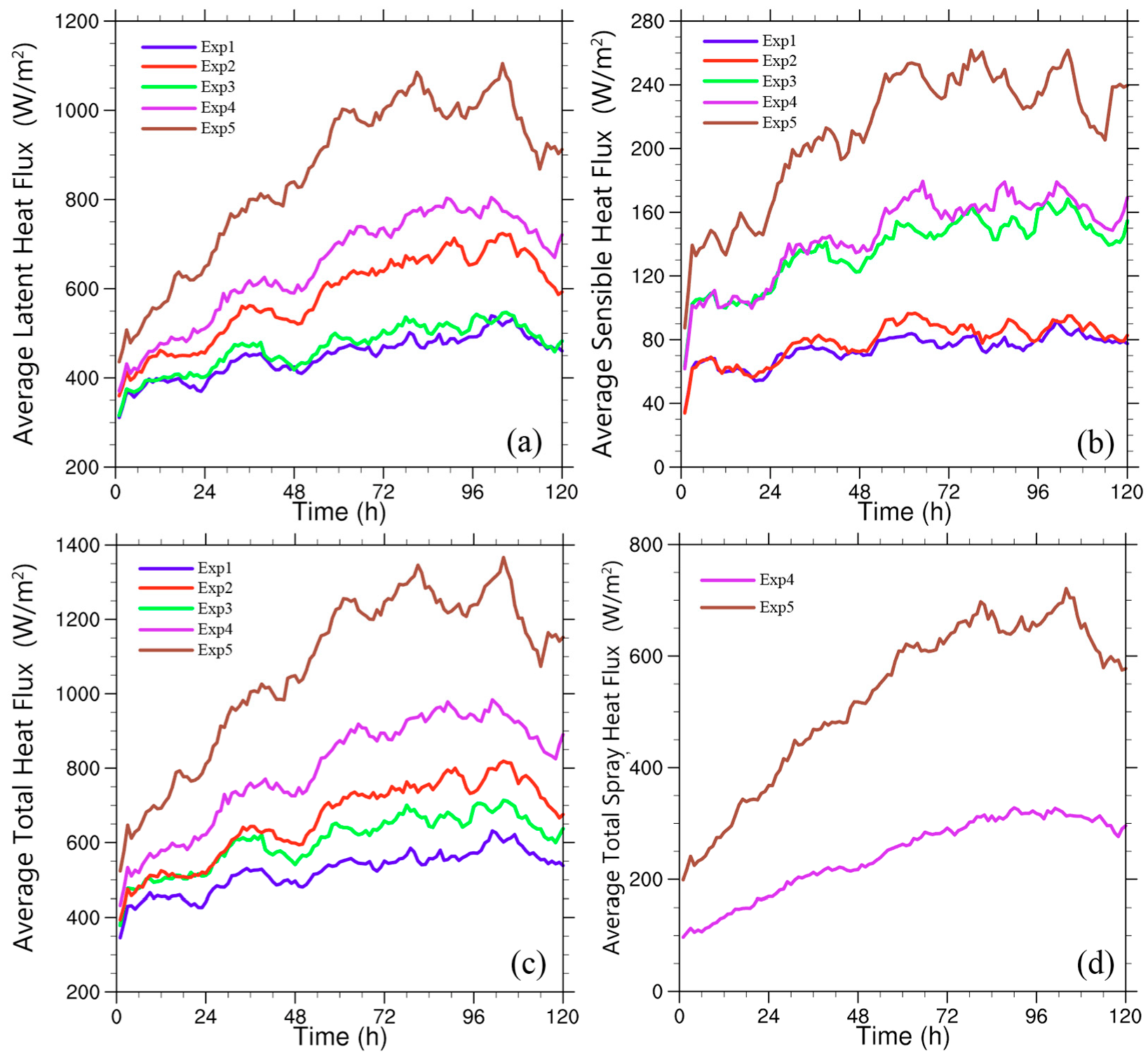
5.3. Heat Flux Analysis of TC
6. Summary and Conclusions
Author Contributions
Funding
Institutional Review Board Statement
Informed Consent Statement
Data Availability Statement
Acknowledgments
Conflicts of Interest
References
- Chen, A.; Giese, M.; Chen, D. Flood impact on Mainland Southeast Asia between 1985 and 2018—The role of tropical cyclones. J. Flood Risk Manag. 2020, 13, e12598. [Google Scholar] [CrossRef]
- Landsea, C.W.; Cangialosi, J.P. Have We Reached the Limits of Predictability for Tropical Cyclone Track Forecasting? Bull. Am. Meteorol. Soc. 2018, 99, 2237–2243. [Google Scholar] [CrossRef]
- Rappaport, E.N.; Jiing, J.-G.; Landsea, C.W.; Murillo, S.T.; Franklin, J.L. The Joint Hurricane Test Bed: Its first decade of tropical cyclone research-to-operations activities reviewed. Bull. Am. Meteorol. Soc. 2012, 93, 371–380. [Google Scholar] [CrossRef]
- Chen, Y.; Zhang, F.; Green, B.W.; Yu, X. Impacts of ocean cooling and reduced wind drag on Hurricane Katrina (2005) based on numerical simulations. Mon. Weather Rev. 2018, 146, 287–306. [Google Scholar] [CrossRef]
- Craig, G.C.; Gray, S.L. CISK or WISHE as the mechanism for tropical cyclone intensification. J. Atmos. Sci. 1996, 53, 3528–3540. [Google Scholar] [CrossRef]
- Ma, Z.; Fei, J.; Huang, X.; Cheng, X. Contributions of Surface Sensible Heat Fluxes to Tropical Cyclone. Part I: Evolution of Tropical Cyclone Intensity and Structure. J. Atmos. Sci. 2015, 72, 120–140. [Google Scholar] [CrossRef]
- Ma, Z.; Fei, J.; Cheng, X.; Wang, Y.; Huang, X. Contributions of Surface Sensible Heat Fluxes to Tropical Cyclone. Part II: The Sea Spray Processes. J. Atmos. Sci. 2015, 72, 4218–4236. [Google Scholar] [CrossRef]
- Zhang, F.; Emanuel, K. On the Role of Surface Fluxes and WISHE in Tropical Cyclone Intensification. J. Atmos. Sci. 2016, 73, 2011–2019. [Google Scholar] [CrossRef]
- Shen, L.-Z.; Wu, C.-C.; Judt, F. The Role of Surface Heat Fluxes on the Size of Typhoon Megi (2016). J. Atmos. Sci. 2021, 78, 1075–1093. [Google Scholar] [CrossRef]
- Emanuel, K.A. An air-sea interaction theory for tropical cyclones. Part I: Steady-state maintenance. J. Atmos. Sci. 1986, 43, 585–605. [Google Scholar] [CrossRef]
- Rotunno, R.; Emanuel, K.A. An air-sea interaction theory for tropical cyclones. Part II: Evolutionary study using a nonhydrostatic axisymmetric numerical model. J. Atmos. Sci. 1987, 44, 542–561. [Google Scholar] [CrossRef]
- Fairall, C.W.; Bradley, E.F.; Hare, J.; Grachev, A.A.; Edson, J.B. Bulk parameterization of air–sea fluxes: Updates and verification for the COARE algorithm. J. Clim. 2003, 16, 571–591. [Google Scholar] [CrossRef]
- Andreas, E.L.; Mahrt, L.; Vickers, D. An improved bulk air–sea surface flux algorithm, including spray-mediated transfer. Q. J. R. Meteorol. Soc. 2015, 141, 642–654. [Google Scholar] [CrossRef]
- Smith, S.D.; Katsaros, K.B.; Oost, W.A.; Mestayer, P.G. Two major experiments in the Humidity Exchange over the Sea (HEXOS) program. Bull. Am. Meteorol. Soc. 1990, 71, 161–172. [Google Scholar] [CrossRef]
- Friehe, C.A.; Schmitt, K.F. Parameterization of air-sea interface fluxes of sensible heat and moisture by the bulk aerodynamic formulas. J. Phys. Oceanogr. 1976, 6, 801–809. [Google Scholar] [CrossRef]
- Geernaert, G. Bulk parameterizations for the wind stress and heat fluxes. In Surface Waves and Fluxes; Springer: Berlin, Germany, 1990; pp. 91–172. [Google Scholar]
- Liu, W.T.; Katsaros, K.B.; Businger, J.A. Bulk parameterization of air-sea exchanges of heat and water vapor including the molecular constraints at the interface. J. Atmos. Sci. 1979, 36, 1722–1735. [Google Scholar] [CrossRef]
- Fairall, C.W.; Bradley, E.F.; Rogers, D.P.; Edson, J.B.; Young, G.S. Bulk parameterization of air-sea fluxes for tropical ocean-global atmosphere coupled-Ocean atmosphere response experiment. J. Geophys. Res. Ocean. 1996, 101, 3747–3764. [Google Scholar] [CrossRef]
- Zeng, X.; Zhao, M.; Dickinson, R.E. Intercomparison of bulk aerodynamic algorithms for the computation of sea surface fluxes using TOGA COARE and TAO data. J. Clim. 1998, 11, 2628–2644. [Google Scholar] [CrossRef]
- Garratt, J.R. The atmospheric boundary layer. Earth-Sci. Rev. 1994, 37, 89–134. [Google Scholar] [CrossRef]
- Wu, J.; Murray, J.J.; Lai, R.J. Production and distributions of sea spray. J. Geophys. Res. Ocean. 1984, 89, 8163–8169. [Google Scholar] [CrossRef]
- Andreas, E.L. Sea spray and the turbulent air-sea heat fluxes. J. Geophys. Res. Ocean. 1992, 97, 11429–11441. [Google Scholar] [CrossRef]
- Rizza, U.; Canepa, E.; Ricchi, A.; Bonaldo, D.; Carniel, S.; Morichetti, M.; Passerini, G.; Santiloni, L.; Scremin Puhales, F.; Miglietta, M.M. Influence of Wave State and Sea Spray on the Roughness Length: Feedback on Medicanes. Atmosphere 2018, 9, 301. [Google Scholar] [CrossRef]
- Andreas, E.L.; Emanuel, K.A. Effects of sea spray on tropical cyclone intensity. J. Atmos. Sci. 2001, 58, 3741–3751. [Google Scholar] [CrossRef]
- Andreas, E.L. Fallacies of the enthalpy transfer coefficient over the ocean in high winds. J. Atmos. Sci. 2011, 68, 1435–1445. [Google Scholar] [CrossRef]
- Andreas, E.L. Spray-mediated enthalpy flux to the atmosphere and salt flux to the ocean in high winds. J. Phys. Oceanogr. 2010, 40, 608–619. [Google Scholar] [CrossRef]
- Shpund, J.; Khain, A.; Rosenfeld, D. Effects of Sea Spray on the Dynamics and Microphysics of an Idealized Tropical Cyclone. J. Atmos. Sci. 2019, 76, 2213–2234. [Google Scholar] [CrossRef]
- Andreas, E.L. 3.4 An Algorithm to Predict the Turbulent Air-Sea Fluxes in High-Wind, Spray Conditions. Environmental Science. 2003. Available online: https://ams.confex.com/ams/annual2003/techprogram/paper_52221.htm (accessed on 14 September 2022).
- Warner, J.C.; Armstrong, B.; He, R.; Zambon, J.B. Development of a coupled ocean–atmosphere–wave–sediment transport (COAWST) modeling system. Ocean Model. 2010, 35, 230–244. [Google Scholar] [CrossRef]
- Joly, A.; Browning, K.A.; Bessemoulin, P.; Cammas, J.P.; Caniaux, G.; Chalon, J.P.; Clough, S.A.; Dirks, R.; Emanuel, K.A.; Eymard, L. Overview of the field phase of the Fronts and Atlantic Storm-Track EXperiment (FASTEX) project. Q. J. R. Meteorol. Soc. 1999, 125, 3131–3163. [Google Scholar] [CrossRef]
- Eymard, L.; Caniaux, G.; Dupuis, H.; Prieur, L.; Giordani, H.; Troadec, R.; Bessemoulin, P.; Lachaud, G.; Bouhours, G.; Bourras, D. Surface fluxes in the North Atlantic current during CATCH/FASTEX. Q. J. R. Meteorol. Soc. 1999, 125, 3563–3599. [Google Scholar] [CrossRef]
- Joly, A.; Jorgensen, D.; Shapiro, M.A.; Thorpe, A.; Bessemoulin, P.; Browning, K.A.; Cammas, J.-P.; Chalon, J.-P.; Clough, S.A.; Emanuel, K.A. The Fronts and Atlantic Storm-Track Experiment (FASTEX): Scientific objectives and experimental design. Bull. Am. Meteorol. Soc. 1997, 78, 1917–1940. [Google Scholar] [CrossRef]
- Persson, P.O.G.; Hare, J.; Fairall, C.; Otto, W. Air-sea interaction processes in warm and cold sectors of extratropical cyclonic storms observed during FASTEX. Q. J. R. Meteorol. Soc. 2005, 131, 877–912. [Google Scholar] [CrossRef]
- Anctil, F.; Donelan, M.A.; Drennan, W.M.; Graber, H.C. Eddy-correlation measurements of air-sea fluxes from a discus buoy. J. Atmos. Ocean. Technol. 1994, 11, 1144–1150. [Google Scholar] [CrossRef]
- Jacob, R.; Larson, J.; Ong, E. M × N communication and parallel interpolation in Community Climate System Model Version 3 using the model coupling toolkit. Int. J. High Perform. Comput. Appl. 2005, 19, 293–307. [Google Scholar] [CrossRef]
- Porchetta, S.; Temel, O.; Warner, J.C.; Muñoz-Esparza, D.; Monbaliu, J.; van Beeck, J.; van Lipzig, N. Evaluation of a roughness length parametrization accounting for wind–wave alignment in a coupled atmosphere–wave model. Q. J. R. Meteorol. Soc. 2021, 147, 825–846. [Google Scholar] [CrossRef]
- Zambon, J.B.; He, R.; Warner, J.C. Investigation of hurricane Ivan using the coupled ocean–atmosphere–wave–sediment transport (COAWST) model. Ocean Dyn. 2014, 64, 1535–1554. [Google Scholar] [CrossRef]
- Bruneau, N.; Toumi, R.; Wang, S. Impact of wave whitecapping on land falling tropical cyclones. Sci. Rep. 2018, 8, 652. [Google Scholar] [CrossRef]
- Ricchi, A.; Bonaldo, D.; Cioni, G.; Carniel, S.; Miglietta, M.M. Simulation of a flash-flood event over the Adriatic Sea with a high-resolution atmosphere–ocean–wave coupled system. Sci. Rep. 2021, 11, 9388. [Google Scholar] [CrossRef]
- Zou, L.; Zhou, T. A Review of Development and Application of Regional Ocean-Atmosphere Coupled Model. Adv. Earth Sci. 2012, 27, 857–865. [Google Scholar]
- Sun, D.; Song, J.; Leng, H.; Ren, K.; Li, X. Impacts of Air-Sea Energy Transfer on Typhoon Modelling. Adv. Meteorol. 2021, 2021, 5567717. [Google Scholar] [CrossRef]
- Chen, S.-H.; Sun, W.-Y. A one-dimensional time dependent cloud model. J. Meteorol. Soc. Japan. Ser. II 2002, 80, 99–118. [Google Scholar] [CrossRef]
- Iacono, M.J.; Delamere, J.S.; Mlawer, E.J.; Shephard, M.W.; Clough, S.A.; Collins, W.D. Radiative forcing by long-lived greenhouse gases: Calculations with the AER radiative transfer models. J. Geophys. Res. Atmos. 2008, 113. [Google Scholar] [CrossRef]
- Nakanishi, M.; Niino, H. Development of an improved turbulence closure model for the atmospheric boundary layer. J. Meteorol. Soc. Japan. Ser. II 2009, 87, 895–912. [Google Scholar] [CrossRef]
- Ek, M.; Mitchell, K.; Lin, Y.; Rogers, E.; Grunmann, P.; Koren, V.; Gayno, G.; Tarpley, J. Implementation of Noah land surface model advances in the National Centers for Environmental Prediction operational mesoscale Eta model. J. Geophys. Res. Atmos. 2003, 108. [Google Scholar] [CrossRef]
- Kain, J.S. The Kain–Fritsch convective parameterization: An update. J. Appl. Meteorol. 2004, 43, 170–181. [Google Scholar] [CrossRef]
- Boijj, N.; Ris, R.; Holthuijsen, L. A third generation wave model for coastal regions; part I: Model description and validation. J. Geophys. Res 1999, 104, 7649–7666. [Google Scholar] [CrossRef]
- Andreas, E.L. Time constants for the evolution of sea spray droplets. Tellus B 1990, 42, 481–497. [Google Scholar] [CrossRef]
- Andreas, E.L. Approximation formulas for the microphysical properties of saline droplets. Atmos. Res. 2005, 75, 323–345. [Google Scholar] [CrossRef]
- Andreas, E.L. A review of the sea spray generation function for the open ocean. Adv. Fluid Mech. 2002, 33, 1–46. [Google Scholar]
- Fairall, C. The effect of sea spray on surface energy transports over the ocean. Glob. Atmos. Ocean Syst. 1994, 2, 121. [Google Scholar]
- Andreas, E.L.; Decosmo, J. Sea spray production and influence on air-sea heat and moisture fluxes over the open ocean. In Air-Sea Exchange: Physics, Chemistry and Dynamics; Springer: Berlin, Germany, 1999; pp. 327–362. [Google Scholar]
- Andreas, E.L.; Decosmo, J. The signature of sea spray in the HEXOS turbulent heat flux data. Bound.-Layer Meteorol. 2002, 103, 303–333. [Google Scholar] [CrossRef]
- Andreas, E.L.; Persson, P.O.G.; Hare, J.E. A bulk turbulent air–sea flux algorithm for high-wind, spray conditions. J. Phys. Oceanogr. 2008, 38, 1581–1596. [Google Scholar] [CrossRef]
- Wang, H.; Yang, Y.; Dong, C.; Su, T.; Sun, B.; Zou, B. Validation of an Improved Statistical Theory for Sea Surface Whitecap Coverage Using Satellite Remote Sensing Data. Sensors 2018, 18, 3306. [Google Scholar] [CrossRef] [PubMed]
- Hwang, P.A. High-wind drag coefficient and whitecap coverage derived from microwave radiometer observations in tropical cyclones. J. Phys. Oceanogr. 2018, 48, 2221–2232. [Google Scholar] [CrossRef]
- Andreas, E.L.; Mahrt, L.; Vickers, D. A new drag relation for aerodynamically rough flow over the ocean. J. Atmos. Sci. 2012, 69, 2520–2537. [Google Scholar] [CrossRef]
- Prakash, K.R.; Pant, V.; Nigam, T. Effects of the Sea Surface Roughness and Sea Spray-Induced Flux Parameterization on the Simulations of a Tropical Cyclone. J. Geophys. Res. Atmos. 2019, 124, 14037–14058. [Google Scholar] [CrossRef]
- Olabarrieta, M.; Warner, J.C.; Armstrong, B.; Zambon, J.B.; He, R. Ocean-atmosphere dynamics during Hurricane Ida and Nor’Ida: An application of the coupled ocean-atmosphere-wave-sediment transport (COAWST) modeling system. Ocean Model. 2012, 43, 112–137. [Google Scholar] [CrossRef]
- Chen, H.; Zhang, D.-L. On the rapid intensification of Hurricane Wilma (2005). Part II: Convective bursts and the upper-level warm core. J. Atmos. Sci. 2013, 70, 146–162. [Google Scholar] [CrossRef]
- Tang, X.; Ping, F.; Yang, S.; Li, M.; Peng, J. Relationship between convective bursts and the rapid intensification of Typhoon Mujigae (2015). Atmos. Sci. Lett. 2018, 19, e811. [Google Scholar] [CrossRef]
- Bender, M.A.; Ginis, I. Real-case simulations of hurricane–ocean interaction using a high-resolution coupled model: Effects on hurricane intensity. Mon. Weather Rev. 2000, 128, 917–946. [Google Scholar] [CrossRef]
- Zhao, B.; Qiao, F.; Cavaleri, L.; Wang, G.; Bertotti, L.; Liu, L. Sensitivity of typhoon modeling to surface waves and rainfall. J. Geophys. Res. Ocean. 2017, 122, 1702–1723. [Google Scholar] [CrossRef]
- Li, F.-N.; Song, J.-B.; He, H.-L.; Li, S.; Li, X.; Guan, S.-D. Assessment of surface drag coefficient parametrizations based on observations and simulations using the Weather Research and Forecasting model. Atmos. Ocean. Sci. Lett. 2016, 9, 327–336. [Google Scholar] [CrossRef]
- Green, B.W.; Zhang, F. Impacts of air–sea flux parameterizations on the intensity and structure of tropical cyclones. Mon. Weather Rev. 2013, 141, 2308–2324. [Google Scholar] [CrossRef] [Green Version]


| EXP ID | EXP Name | a | b |
|---|---|---|---|
| 1 | L0_S0 | 0 | 0 |
| 2 | L1_S0 | 1 | 0 |
| 3 | L0_S1 | 0 | 1 |
| 4 | L1_S1 | 1 | 1 |
| 5 | L2_S2 | 2 | 2 |
| Exp ID | Exp Name | MSLP | VMAX | ||
|---|---|---|---|---|---|
| RMSE | S | RMSE | S | ||
| 1 | L0_S0 | 37.09 | 0.24 | 18.67 | 0.19 |
| 2 | L1_S0 | 25.08 | 0.53 | 12.74 | 0.46 |
| 3 | L0_S1 | 34.98 | 0.27 | 17.88 | 0.21 |
| 4 | L1_S1 | 19.38 | 0.69 | 9.37 | 0.67 |
| 5 | L2_S2 | 16.29 | 0.80 | 7.27 | 0.79 |
Publisher’s Note: MDPI stays neutral with regard to jurisdictional claims in published maps and institutional affiliations. |
© 2022 by the authors. Licensee MDPI, Basel, Switzerland. This article is an open access article distributed under the terms and conditions of the Creative Commons Attribution (CC BY) license (https://creativecommons.org/licenses/by/4.0/).
Share and Cite
Lan, Y.; Leng, H.; Sun, D.; Song, J.; Cao, X. An Improved Sea Spray-Induced Heat Flux Algorithm and Its Application in the Case Study of Typhoon Mangkhut (2018). J. Mar. Sci. Eng. 2022, 10, 1329. https://doi.org/10.3390/jmse10091329
Lan Y, Leng H, Sun D, Song J, Cao X. An Improved Sea Spray-Induced Heat Flux Algorithm and Its Application in the Case Study of Typhoon Mangkhut (2018). Journal of Marine Science and Engineering. 2022; 10(9):1329. https://doi.org/10.3390/jmse10091329
Chicago/Turabian StyleLan, Yunjie, Hongze Leng, Difu Sun, Junqiang Song, and Xiaoqun Cao. 2022. "An Improved Sea Spray-Induced Heat Flux Algorithm and Its Application in the Case Study of Typhoon Mangkhut (2018)" Journal of Marine Science and Engineering 10, no. 9: 1329. https://doi.org/10.3390/jmse10091329