Extended State Observer-Based Parameter Identification of Response Model for Autonomous Vessels

Abstract

Identification of parameters involved in the linear response model with high precision is a highly cost-effective, as well as a challenging task, in developing a suitable model for the verification and validation (V+V) of some key techniques for autonomous vessels in the virtual testbed, e.g., guidance, navigation, and control (GNC). In order to deal with this identification problem, a novel identification framework is proposed in this paper by introducing the extended state observer (ESO), and the well-evaluated robust weighted least square support vector regression algorithm (RW-LSSVR). A second-order linear response model is investigated in this study due to its wide use in controller designs. Considering the highly possible situation that only limited states could be measured directly, the required but immeasurable states in identifying parameters contained in the response model are approximately estimated by the ESO. Theoretical analysis of the stability is given to show and improve the applicability of the ESO. Simulation studies based on linear response models with predefined parameter values of a cargo vessel and a patrol vessel maneuvering in an open water area are carried out, respectively. Results show that the proposed approach not only estimates immeasurable states with high accuracy but also ensures good performance on the parameter identification of the response model with very close values to the nominal ones. The proven identified approach is economic because it only requires limited kinds of low-cost sensors.

1. Introduction

1.1. Motivation

As a multi-billion industry controlling 90% of all world trade, the shipping community is continuously striving for improved operational margins while preserving and enhancing human and environmental safety standards. Technology availability implies that autonomy concepts could prove useful in terms of tackling challenges associated with ocean-based transportation by 2030 or earlier. Autonomous vessels could reduce challenges due to human error and increase profit margins assuming that risks associated with security, operations, and the emergence of technologies (e.g., machine learning, artificial intelligence, sensors) are well mitigated by sound performance-driven standards. The well-known leading three autonomous vessel technology development projects include MUNIN (Maritime Unmanned Navigation through Intelligence in Networks), DNV GLReVolt, and YARA Birkeland [1]. These projects are significantly dedicated to developing autonomous vessels mainly due to the economic and service-related benefits. For instance, autonomous vessels contribute significantly to improving maritime safety by reducing the number of fatalities [2], the likelihood of collision [3], and the vulnerability to piracy [4]. On top of the profit of autonomous vessels, the major contribution is the reduction of the environmental impacts of shipping both directly and indirectly [1].

Many technical tasks involving for example guidance, navigation, and control (GNC) relevant to the development of autonomous vessels are required to be tested effectively before final field applications [5]. For the design of the controller and corresponding tests, it is of significant importance to adopt a suitable dynamic model under the consideration of the trade-off between model accuracy and model complexity [6]. The data-fitting accuracy depends on the model selection. The involvement of complex higher-order terms and more coefficients improves the description reality of ship dynamics. However, it results in the coupling and nonlinearity of the parameter drift becoming more serious. Additionally, the computational costs would be increased, making the identification more difficult. Therefore, a suitable model should well present the system dynamics and keep a satisfactory computational speed by neglecting the unnecessary high-order terms and coefficients.

1.2. Related Work

Up to date, four kinds of such models are able to be applicable for model-based control design, i.e., the holistic version, also called the Abkowitz model, the modular type named the mathematical modeling group (MMG) model, the vectorial representation model, and the response model or the Nomoto model [7]. In reality, it is much more effective to operate a response system instead of adjusting the vessel thrust system to control vessels according to the practical sailing experience of crews and captains. The high inertia of vessels leads to a faster reaction of the response system than the thrust system. Therefore, the control task is usually tracked by adjusting the vessel heading with the use of a suitable response model under the assumption of constant vessel speed [8]. Apart from the determination of the structure of the response model, an additional key aspect is the estimation of parameters involved in the response model.

A variety of techniques regarding parameter estimation of vessel dynamic models, which are also applicable for the response model issue, have been studied [6,9,10,11,12,13], and can be classified into three typical techniques, i.e., the captive model tests technique [12], the computational fluid dynamics (CFD) based method [11,13], the system identification with full-scale model trails, and free-running tests including parametric and non-parametric tricks [6,10]. The captive model tests technique can be applied with the requirement of a set of large facilities and professional operators. The computational fluid dynamics (CFD)-based method can be treated as an effective way but it has a high computational cost. Comparatively, the system identification technique can always ensure superior performance on model parameter estimation due to its highly attractive cost-effectiveness and satisfactory identification results with relatively low efforts committed to carrying out vessel maneuver trails and data measurements.

In terms of implementing parameter identification for autonomous vessels based on system identification techniques, attention should be paid to completing four correlated procedures i.e., data collection, model determination, identification method development, and model validation [14]. Data extracted from optimal experiments should be sufficiently informative to guarantee the convergence and robustness of the identification approach [15]. Some researchers have studied the design of experiment (DOE) for setting up optimal experiments [16]. For instance, ref. [16] proposed an optimization idea by combining a multi-level pseudo-random sequence, the D-optimality criteria, and ant colony optimization algorithm to obtain optimized excitation signals used to determine the training data. Compared to widely used zigzag maneuver signals, the application of optimized signals can reduce the variance of parameters and improve the generalization ability of the identified model, especially in presence of environmental disturbances and measurement noises, but the efficiency of the designed approach in particular in terms of the convergence rate is not so satisfactory. In the case of model determination, the above classification of four typical dynamic models is a potential selection.

This paper focuses on the identification of the response model, which is significant to controller designs for autonomous vessels. A number of identification methods have been investigated.

Table 1. Comparative analysis of the identification methods.

Method	Advantage	Disadvantage	Typical Study
LS	1. easy to implement	1. sensitive to outliers	[17]
	2. wide applications	2. inconsistent estimates
NLS	1. approximate linearization of the objective function	1. identification value is unstable	[24]
	2. fast convergence, easy to implement	2. local optimum
KF	1. has a certain robustness	1. external excitation is needed to be known	[18]
	2. strong versatility	2. linearized dynamic systems make it difficult to apply to nonlinear systems
		3. initial value dependence
GPR	1. working well on small datasets	1. low sparsity	[20]
	2. provide uncertainty measurements on the predictions	2. suitable initialization is required
BAS	simple and efficient	not stable	[21]
CMA-ES	applicable to nonlinear or non-convex continuous optimization problems	reasonable initialization is required to ensure its optimization performance, but hard to do	[22]
NI	1. has a certain robustness	multi-innovation matrix inversion results in a large amount of computation	[23]
	2. converges faster for a certain input dimension
SVM	1. has satisfactory robustness	1. low sparsity of the solution	[19]
	2. guarantees global optimum	2. some parameters need to be optimized reasonably
$\nu$-SVM	1. suitable for the nonlinear dynamic systems	1. parameter drift problem	[25]
	2. easy to perform parameter optimization	2. lowly applicable to strong nonlinear systems
RW-LSSVR	1. robust to the condition with disturbance	low sparsity of the solution	[6]
	2. optimal initialization

gives the comparative analysis of these methods, for instance, the least square (LS) method [17], Kalman filter (KF) method [18], support vector machines (SVM) [19], Gaussian process regression algorithm (GPR) [20], beetle antenna search (BAS) algorithm [21], covariance matrix adaptation evolution strategy (CMA-ES) [22], and nonlinear innovation algorithm (NI) [23]. Moreover, some relevant modified approaches are further developed to overcome their underlying deficiencies. For example, the nonlinear LS (NLS) method is proposed to handle the ill-conditioned problem of the LS [24]. To alleviate the impact of noise-induced problems, such as parameter drift or over-fitting, on the model reliability, the $\nu$-SVM method is developed to identify the ship maneuvering model [25]. This method can automatically control the number of support vectors to ensure the sparsity of the solution. The robust weighted least square support vector regression algorithm (RW-LSSVR) advanced with the purpose of particularly setting structural parameters involved in the least square support vector regression algorithm (LS-SVR) and reducing the impacts of noises on identification results [6].

The training data and validation data extracted at the data collection stage have conclusive effects on the success of the identification results [26,27]. Correspondingly, the prominent issue mainly concerning the DOE to obtain maximum informative excitation, which has been investigated in the literature [15,16], deserves careful attention. However, these works are carried out with the assumption that all states required for identification are available in two ways, i.e., directly measuring, and indirect differentiation using direct measurements. It is noticeable that the latter way could introduce accumulative errors if some high-order states existed, which is not expected in the identification procedure. Therefore, one major focus of this study is how to overcome this tough problem, i.e., how to effectively acquire the states, especially the indirectly measured ones for parameter identification using low-cost sensors.

One inspiration to deal with this concern is derived from the active disturbance rejection control direction, in which the total disturbances are considered as an additional state variable that is estimated by an observer from the measured input/output data and compensated in real time [28,29,30,31,32]. Many methods can be used as the observer, such as the extended state observer (ESO) [29,30,33], Luenberger observer (LO) [34,35], sliding mode observer (SMO) [36], distributed event-triggered observer (DETO) [37], high-gain observer (HGO) [38], fuzzy state observer (FSO) [39], and the Kalman filter (KF) and its related modified versions [40].

Table 2. Comparative analysis of the observers.

Observer	Advantage	Disadvantage	Typical Study
ESO	straightforward to implement	suitable settings of gains are required	[29,30,33]
LO	simple design	restricted to the deterministic case	[34,35]
KF	used for the stochastic case	not all states can be estimated	[40]
SMO	has a strong robustness	suffers from the chattering problem.	[36]
HGO	simple structure and easy tuning	sensitive to existing measurement noise	[38]
FSO	flexible design	the gain vector requires strict setting	[39]
DETO	applicable to the high-order uncertain nonlinear systems	relatively high computational cost	[37]

illustrates the comparative analysis of the observers. The studies point out that the ESO is the most suitable for observing systems with unknown rates of state change while comparing to the other observers. In addition, the ESO is also able to construct the correction term with the use of the reaching laws of LO or SMO. Therefore, the ESO is comparatively more suitable for this study due to its superior characteristics which can be summarized as follows. (1) It has little dependence on the exact mathematical model of the system [33]. (2) It is straightforward to implement [29]. (3) The performance of the controller with ESO can be greatly improved [30]. The observer can estimate the immeasurable states under the condition of various disturbances.

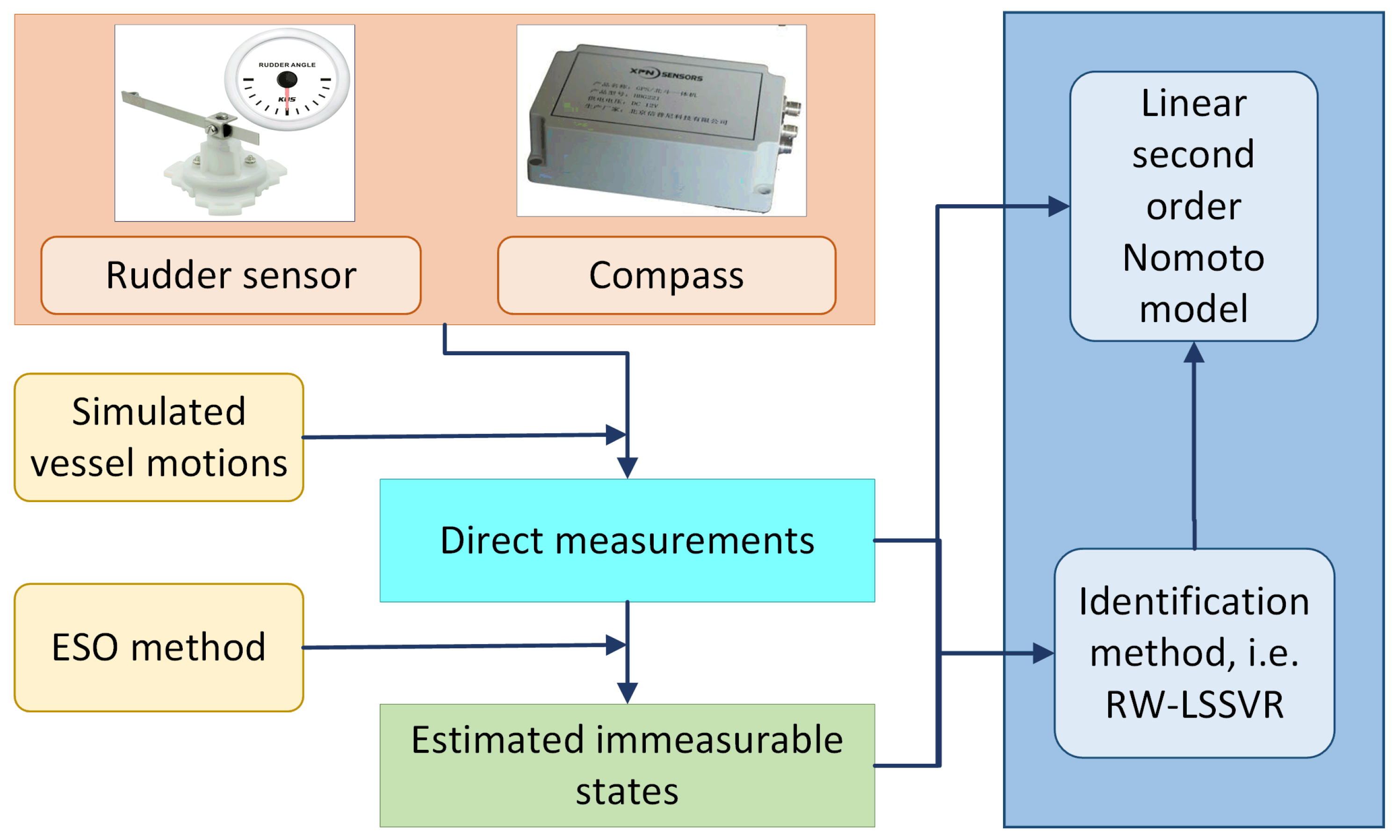
1.3. The Overview of the Framework Regarding the Proposed Identification Approach

In this paper, the ESO incorporated with RW-LSSVR is proposed for the parameter identification of the response model for autonomous vessels. The response model of autonomous vessels expressed in the linear second-order form is regarded as the investigated model. Some immeasurable states are estimated by the ESO with direct measurements such as the rudder angle logged by the rudder sensor and the heading angle recorded by the compass. The RW-LSSVR method developed and effectively evaluated in our previous study [6] is applied in this work as a response model parameters identifier. In the end, the samples stemmed from dynamic simulations using a linear response model with predetermined parameter values and persistent activation are utilized for verification and validation of the proposed parameter identification approach. Figure 1 shows the overview of the framework of the proposed hybrid identification approach.

1.4. Contribution

The main contributions of the present paper are: (1) a novel identification framework is proposed by benefiting from the extended state observer (ESO) for tackling immeasurable states and the previously well-evaluated robust weighted least square support vector regression algorithm (RW-LSSVR). (2) With the limitations of financial support as well as available sensors, it is not always guaranteed to acquire all required states directly and accurately. Some states required for identification are logged using low-cost sensors directly. Other immeasurable states are calculated by the ESO only employing the measured states with low cost. To the best of the authors’ knowledge, this issue highly associated with the parameter identification technique is seldom addressed in related research.

1.5. Structure of the Paper

The outline of the paper is as follows. The generalized linear response model and its state-space version for autonomous vessels are illustrated in Section 2. The research methodology for the hybrid identification approach is given in Section 3. Section 4 shows the comparative results through simulations. Some remarkable conclusions and future works are given in Section 5.

2. Linear Response Model

In general, four categories of Nomoto models, including the first-order linear and nonlinear versions and the second-order linear and nonlinear versions, are commonly used to describe the heading dynamics with respect to rudder command. The linear models are straightforward for applications in controller design. Comprehensively considering that the response model would be further applicable to design controller with expected high accuracy for complicated autonomous vessel motions [8,41,42], the second-order linear Notomo model is investigated, which is presented with respect to the heading angle $\left(\psi \left(t\right)\right)$ of autonomous vessels.

$${\displaystyle \stackrel{⃛}{\psi }\left(t\right)+\left(\frac{1}{T_1}+\frac{1}{T_2}\right)\ddot{\psi }\left(t\right)+\frac{1}{T_1{T}_2}\dot{\psi }\left(t\right)=\frac{K_R}{T_1{T}_2}\left(T_3\dot{{\delta }_R}\left(t\right)+{\delta }_R\left(t\right)\right)}$$

(1)

in which ${\delta }_R$ donates the rudder angle, $T_1,T_2,T_3,K_R$ are vessel response system parameters.

State space model. As the ESO will be used to estimate some states based on the above introduced nonlinear response model, Equation (1) is converted into a state-space expression given by

$$\left\{\begin{array}{c}\dot{{\mathbf{X}}_{\mathbf{ss}}}={\mathbf{AX}}_{\mathbf{ss}}+{\mathbf{Bu}}_{\mathbf{ss}}\hfill \\ {\mathbf{Y}}_{\mathbf{ss}}={\mathbf{CX}}_{\mathbf{ss}}+{\mathbf{Du}}_{\mathbf{ss}}\hfill \end{array}\right.$$

(2)

where the system state vector is ${\displaystyle {\mathbf{X}}_{\mathbf{ss}}={\left[x_{ss1}{x}_{ss2}{x}_{ss3}\right]}^T={\left[\psi \left(t\right)\dot{\psi \left(t\right)}\ddot{\psi }\left(t\right)\right]}^T}$, the system output vector is ${\displaystyle {\mathbf{Y}}_{\mathbf{ss}}=\left[y_{ss}\right]=\left[x_{ss1}\right]}$, the system input vector is ${\mathbf{u}}_{\mathbf{ss}}={\left[u_{ss1}{u}_{ss2}\right]}^T={\left[\dot{{\delta }_R}\left(t\right){\delta }_R\left(t\right)\right]}^T$, the system state matrix is ${\displaystyle \mathbf{A}=\left[\begin{array}{ccc}0& 1& 0\\ 0& 0& 1\\ 0& -a_1& -a_1{a}_2\end{array}\right]}$, the system input matrix is ${\displaystyle \mathbf{B}=\left[\begin{array}{cc}0& 0\\ 0& 0\\ a_1{a}_3{a}_4& a_1{a}_3\end{array}\right]}$, and the system output matrix is ${\displaystyle \mathbf{C}=\left[100\right]}$, and ${\displaystyle \mathbf{D}=\left[00\right]}$, where ${\displaystyle a_1=\frac{1}{T_1{T}_2}}$, $a_2=T_1+T_2$, $a_3=K_R$, $a_4=T_3$.

With the consideration of the response characteristics of autonomous vessels, the following assumption is made.

Assumption 1.

The steering gear system of autonomous vessels satisfies the first-order linear response relationship with the response time of $T_m$, which can be formulated as

$${\displaystyle \dot{{\delta }_R}\left(t\right)=\frac{1}{T_m}{\delta }_R\left(t\right)+\frac{1}{T_m}{\delta }_{Rset}\left(t\right).}$$

(3)

To construct a reasonable state-space model for autonomous vessels, the combination of the steering gear system with the original state-space model in Equation (2) is done. The time-continuous rudder angle is regarded as a state. For the sake of convenience of applying ESO, the original state vector is renewed to be $\mathbf{X}$ with states $x_1=\psi \left(t\right)$, $x_2=\dot{\psi }\left(t\right)$, $x_3={\delta }_R\left(t\right)$, $x_4=\ddot{\psi }\left(t\right)$, and the input is $u_{temp}={\delta }_{Rset}\left(t\right)$. Therefore, the state-space formulate in Equation (2) is rewritten to be

$$\left\{\begin{array}{c}{\displaystyle \dot{x_1}=x_2}\hfill \\ {\displaystyle \dot{x_2}=x_4}\hfill \\ {\displaystyle \dot{x_3}=-\frac{1}{T_m}{x}_3+\frac{1}{T_m}{u}_{temp}}\hfill \\ {\displaystyle \dot{x_4}=-a_2{x}_2-(a_1{a}_2+\frac{a_1{a}_3{a}_4}{T_m})x_3+a_1{a}_3{x}_4+\frac{a_1{a}_3{a}_4}{T_m}{u}_{temp}}\hfill \end{array}\right..$$

(4)

After analyzing the steering gear system, it can be found that the system is unstable. Hence, the basic proportional (P) control obtained by briefing conventional proportional–integral–derivative (PID) control is employed to adjust the system to generate a stable response. Afterward, the input in Equation (4) is updated with the gain $k_p$ of the P control as follow

$${\displaystyle u_{temp}=k_p({\psi }_{set}\left(t\right)-x_1),}$$

(5)

where ${\psi }_{set}\left(t\right)$ is the desirable heading angle. Assume that the input is rewritten to be $u={\psi }_{set}\left(t\right)$. Then the expression of Equation (4) can be given as follows.

$$\left\{{\displaystyle \begin{array}{c}{\displaystyle \dot{x_1}=x_2}\hfill \\ {\displaystyle \dot{x_2}=x_4}\hfill \\ {\displaystyle \dot{x_3}=-\frac{k_p}{T_m}{x}_1-\frac{1}{T_m}{x}_3+\frac{k_p}{T_m}u}\hfill \\ \dot{x_4}=-\frac{a_1{a}_3{a}_4{k}_p}{T_m}{x}_1-a_2{x}_2-(a_1{a}_2+\frac{a_1{a}_3{a}_4}{T_m})x_3\hfill \\ +a_1{a}_3{x}_4+\frac{a_1{a}_3{a}_4{k}_p}{T_m}u.\hfill \end{array}}\right.$$

(6)

3. Research Methodology

3.1. State Estimation Based on ESO

The nonlinear ESO has a complex structure and will increase the difficulties of stability analysis. Moreover, more control parameters need to be adjusted and most of them are usually selected by the empirical values [33]. Thus, a linear ESO is adopted.

Assuming that ${\displaystyle p_1=-\frac{a_1{a}_3{a}_4{k}_p}{T_m}}$, $p_2=-a_2$, ${\displaystyle p_3=-a_1{a}_2-\frac{a_1{a}_3{a}_4}{T_m}}$, $p_4=a_1{a}_3$, ${\displaystyle b=\frac{a_1{a}_3{a}_4{k}_p}{T_m}}$, the extended state can be presented as

$${\displaystyle x_5=p_1{x}_1+p_2{x}_2+p_3{x}_3+p_4{x}_4+(b-1)u.}$$

(7)

Correspondingly, $\dot{x_4}=x_5+u$.

Therefore, the linear ESO can be constructed as follows

$$\left\{\begin{array}{c}{\displaystyle \dot{z_1}=z_2+l_1(x_1-z_1)}\hfill \\ {\displaystyle \dot{z_2}=z_4+l_2(x_1-z_1)}\hfill \\ {\displaystyle \dot{z_3}=-\frac{k_p}{T_m}{z}_1-\frac{1}{T_m}{z}_3+\frac{k_p}{T_m}u+l_3(x_1-z_1)}\hfill \\ {\displaystyle \dot{z_4}=z_5+u+l_4(x_1-z_1)}\hfill \\ {\displaystyle \dot{z_5}=l_5(x_1-z_1)}\hfill \end{array}\right.,$$

(8)

where $z_1$ is the estimated heading angle $\psi \left(t\right)$, $z_2$ donates the estimated yaw rate $\dot{\psi }\left(t\right)$, $z_3$ presents the estimated rudder angle ${\delta }_R\left(t\right)$, $z_4$ means the estimated acceleration of yaw rate $\ddot{\psi }\left(t\right)$, $z_5$ describes the estimated lumped disturbances, and $l_1,l_2,l_3,l_4,l_5$ are the observer gains closely related to the control performance of the observer.

The corresponding state-space model of the ESO can be given as

$${\displaystyle \frac{d\mathbf{Z}}{dt}={\mathbf{A}}_z\mathbf{Z}+{\mathbf{B}}_z{u}_z+\mathbf{L}({\mathbf{X}}_z-\mathbf{Z})}$$

(9)

where ${\displaystyle \mathbf{Z}={\left[z_1{z}_2{z}_3{z}_4{z}_5\right]}^T}$, ${\mathbf{u}}_z=\left[u\right]=\left[{\psi }_{set}\left(t\right)\right]$, ${\mathbf{B}}_z={\left[00\frac{k_p}{T_m}10\right]}^T$, ${\mathbf{X}}_z={\left[x_1{x}_2{x}_3{x}_4{x}_5\right]}^T$, ${\displaystyle {\mathbf{A}}_z=\left[\begin{array}{ccccc}0& 1& 0& 0& 0\\ 0& 0& 0& 1& 0\\ -\frac{k_p}{T_m}& 0& -\frac{1}{T_m}& 0& 0\\ 0& 0& 0& 0& 1\\ 0& 0& 0& 0& 0\end{array}\right]}$, $\mathbf{L}=\left[\begin{array}{ccccc}{l}_1& 0& 0& 0& 0\\ l_2& 0& 0& 0& 0\\ l_3& 0& 0& 0& 0\\ l_4& 0& 0& 0& 0\\ l_5& 0& 0& 0& 0\end{array}\right]$.

Before the stability analysis of the ESO closed-loop system expressed in Equation (9), a lemma is presented as follows.

Lemma 1.

The prerequisite for a system to be stable is that the real part of the eigenvalue of the state matrix of the system equation is negative and the imaginary part is zero.

Therefore, the system in Equation (9) would be stable and not exhibit overshoot oscillation if the real part of the eigenvalue of the state matrix $(A-L)$ was negative and the imaginary part was zero.

Stability analysis. As the authors of [43] pointed out, the ESO has been widely used in several applications, but the stability analysis is still an open problem since the ESO has a non-smooth structure, which makes the analysis a difficult task. This part concentrates on performing a convergence analysis for the ESO used in this study.

With the sake of convenience, we assume that ${\displaystyle d_{sys}=-\frac{a_1{a}_3{a}_4{k}_p}{T_m}{x}_1-a_2{x}_2-(a_1{a}_2+\frac{a_1{a}_3{a}_4}{T_m})x_3+a_1{a}_3{x}_4+(\frac{a_1{a}_3{a}_4{k}_p}{T_m}-1)u}$. Consequently, ${\dot{x}}_4$ in Equation (6) can be reconstructed as ${\dot{x}}_4=d_{sys}+u$. Substituting the above new expression into Equation (4), the new state-space model for the vessel response system is described by

$${\displaystyle \dot{\mathbf{X}}=\mathbf{AX}+\mathbf{B}u+\mathbf{F}{d}_{sys}}$$

(10)

where ${\displaystyle \mathbf{X}={\left[\begin{array}{cccc}{x}_1& x_2& x_3& x_4\end{array}\right]}^T={\left[\begin{array}{cccc}\psi \left(t\right)& \dot{\psi \left(t\right)}& {\delta }_R\left(t\right)& \ddot{\psi }\left(t\right)\end{array}\right]}^T}$, $u={\psi }_{set}\left(t\right)$, ${\displaystyle \mathbf{B}={\left[\begin{array}{cccc}0& 0& \frac{k_p}{T_m}& 1\end{array}\right]}^T}$, $\mathbf{F}={\left[\begin{array}{cccc}0& 0& 0& 1\end{array}\right]}^T$, $\mathbf{A}=\left[\begin{array}{cccc}0& 1& 0& 0\\ 0& 0& 0& 1\\ -\frac{k_p}{T_m}& 0& -\frac{1}{T_m}& 0\\ 0& 0& 0& 0\end{array}\right]$.

Discretizing Equation (10) with the interval donated as $\Delta t$, the corresponding expression is obtained as follows

$${\displaystyle \mathbf{X}(k+1)={\mathbf{A}}_d\mathbf{X}\left(k\right)+{\mathbf{B}}_{d}u\left(k\right)+{\mathbf{F}}_d{d}_{sys}\left(k\right)}$$

(11)

in which ${\mathbf{B}}_d=\Delta t\mathbf{B}$, ${\mathbf{F}}_d=\Delta t\mathbf{F}$, ${\mathbf{A}}_d=\mathbf{I}+\Delta t\mathbf{A}=\left[\begin{array}{cccc}1& \Delta t& 0& 0\\ 0& 1& 0& \Delta t\\ {\displaystyle -\frac{\Delta t{k}_p}{T_m}}& 0& {\displaystyle 1-\frac{\Delta t}{T_m}}& 0\\ 0& 0& 0& 1\end{array}\right]$.

For the sake of mathematical convenience, we assume that $q=z_5$, which is further substituted into Equation (9). Then the vector-matrix form of Equation (8) is defined as

$$\left\{\begin{array}{c}{\displaystyle \dot{\mathbf{Z}}=\mathbf{HZ}+\mathbf{D}u+\mathbf{E}q+{\mathbf{L}}_1(x_1-z_1)}\hfill \\ {\displaystyle \dot{q}=l_5(x_1-z_1)}\hfill \end{array}\right.$$

(12)

Then the discretized form of Equation (12) is given as

$$\left\{\begin{array}{c}{\displaystyle \mathbf{Z}(k+1)={\mathbf{H}}_d\mathbf{Z}\left(k\right)+{\mathbf{D}}_{d}u\left(k\right)+{\mathbf{E}}_{d}q\left(k\right)+{\mathbf{L}}_{1d}(x_1\left(k\right)-z_1\left(k\right))}\hfill \\ {\displaystyle q(k+1)=q\left(k\right)-L_{2d}(x_1\left(k\right)-z_1\left(k\right))}\hfill \end{array}\right.$$

(13)

where ${\mathbf{H}}_d={\mathbf{A}}_d$, ${\mathbf{D}}_d={\mathbf{B}}_d$, ${\mathbf{E}}_d={\mathbf{F}}_d$, ${\mathbf{L}}_{1d}={\left[\begin{array}{cccc}\Delta t{l}_1& \Delta t{l}_2& \Delta t{l}_3& \Delta t{l}_4\end{array}\right]}^T$, $L_{2d}=\Delta t{l}_5$.

Let the state error $\mathbf{e}\left(k\right)=\mathbf{X}\left(k\right)-\mathbf{Z}\left(k\right)$. The output error can be calculated through $x_1\left(k\right)-z_1\left(k\right)={\mathbf{C}}_d\mathbf{e}\left(k\right)$ with ${\mathbf{C}}_d={\left[\begin{array}{cccc}1& 0& 0& 0\end{array}\right]}^T$. Consequently, define

$$\begin{array}{cc}{\displaystyle \mathbf{e}(k+1)}\hfill & =\mathbf{X}(k+1)-\mathbf{Z}(k+1)\hfill \\ \hfill & ={\mathbf{A}}_d\mathbf{X}\left(k\right)+{\mathbf{B}}_{d}u\left(k\right)+{\mathbf{F}}_d{d}_{sys}\left(k\right)-{\mathbf{H}}_d\mathbf{Z}\left(k\right)\hfill \\ \hfill & -{\mathbf{D}}_{d}u\left(k\right)-{\mathbf{E}}_{d}q\left(k\right)-{\mathbf{L}}_{1d}{\mathbf{C}}_d\mathbf{e}\left(k\right).\hfill \end{array}$$

(14)

Due to ${\mathbf{A}}_d={\mathbf{H}}_d$, ${\mathbf{B}}_d={\mathbf{D}}_d$, ${\mathbf{F}}_d={\mathbf{E}}_d$, Equation (14) can be modifed into

$$\begin{array}{cc}\mathbf{e}(k+1)\hfill & ={\mathbf{A}}_d(\mathbf{X}\left(k\right)-\mathbf{Z}\left(k\right))+{\mathbf{F}}_d(d_{sys}\left(k\right)-q\left(k\right))-{\mathbf{L}}_{1d}{\mathbf{C}}_d\mathbf{e}\left(k\right)\hfill \\ \hfill & =({\mathbf{A}}_d-{\mathbf{L}}_{1d}{\mathbf{C}}_d)\mathbf{e}\left(k\right)+{\mathbf{F}}_d(d_{sys}\left(k\right)-q\left(k\right)).\hfill \end{array}$$

(15)

Let $g\left(k\right)=d_{sys}\left(k\right)-q\left(k\right)$, then the consecutive expression can be described as follows

$$\begin{array}{cc}g(k+1)\hfill & =d_{sys}(k+1)-q(k+1)\hfill \\ \hfill & =d_{sys}(k+1)-q(k+1)+q\left(k\right)-q\left(k\right)+d_{sys}\left(k\right)-d_{sys}\left(k\right)\hfill \\ \hfill & =g\left(k\right)-L_2{\mathbf{C}}_d\mathbf{e}\left(k\right)+(d_{sys}(k+1)-d_{sys}\left(k\right)).\hfill \end{array}$$

(16)

Combine Equation (15) and Equation (16) together to get a form as follows

$${\displaystyle \left[\begin{array}{c}\mathbf{e}(k+1)\\ g(k+1)\end{array}\right]=\left[\begin{array}{cc}{\mathbf{A}}_d-{\mathbf{L}}_{1d}{\mathbf{C}}_d& {\mathbf{F}}_d\\ -L_{2d}{\mathbf{C}}_d& 1\end{array}\right]\left[\begin{array}{c}\mathbf{e}\left(k\right)\\ g\left(k\right)\end{array}\right]+\left[\begin{array}{c}0\\ d_{sys}(k+1)-d_{sys}\left(k\right).\end{array}\right]}$$

(17)

Let $\mathbf{M}=\left[\begin{array}{cc}{\mathbf{A}}_d-{\mathbf{L}}_{1d}{\mathbf{C}}_d& {\mathbf{F}}_d\\ -L_{2d}{\mathbf{C}}_d& 1\end{array}\right]$. Now the problem of analyzing the stability of the ESO can be defined to be the issue of adjusting the sign of the eigenvalues of the continuous form ${\mathbf{M}}_c$ which is presented as follows

$${\displaystyle {\mathbf{M}}_c=\left[\begin{array}{ccccc}-l_1& 1& 0& 0& 0\\ -l_2& 0& 0& 1& 0\\ {\displaystyle -l_3-\frac{k_p}{T_m}}& 0& {\displaystyle -\frac{1}{T_m}}& 0& 0\\ -l_4& 1& 0& 0& 1\\ -l_5& 0& 0& 0& 0\end{array}\right].}$$

(18)

Convert the expression of ${\mathbf{M}}_c$ into the form $(s\mathbf{I}-{\mathbf{M}}_c)$ by introducing identity matrix $\mathbf{I}$, then we can calculate the determinant of $(s\mathbf{I}-{\mathbf{M}}_c)$ presented as follows

$${\displaystyle det(s\mathbf{I}-{\mathbf{M}}_c)=(s^4+l_1{s}^3+l_2{s}^2+l_{4}s+l_5)(s+\frac{1}{T_m})s^6.}$$

(19)

Let $(s^4+l_1{s}^3+l_2{s}^2+l_{4}s+l_5)(s+\frac{1}{T_m})=0$, then we can get the following results.

$$\left\{\begin{array}{c}{\displaystyle l_1=-{\lambda }_1-{\lambda }_2-{\lambda }_4-{\lambda }_5}\hfill \\ {\displaystyle l_2={\lambda }_1{\lambda }_4+{\lambda }_1{\lambda }_5+{\lambda }_2{\lambda }_4+{\lambda }_1{\lambda }_5+{\lambda }_1{\lambda }_2+{\lambda }_4{\lambda }_5}\hfill \\ {\displaystyle {\lambda }_3=-\frac{1}{T_m}}\hfill \\ {\displaystyle l_4=-{\lambda }_1{\lambda }_4{\lambda }_5-{\lambda }_2{\lambda }_4{\lambda }_5-{\lambda }_1{\lambda }_2{\lambda }_4-{\lambda }_1{\lambda }_2{\lambda }_5}\hfill \\ {\displaystyle l_5={\lambda }_1{\lambda }_2{\lambda }_4{\lambda }_5}\hfill \end{array}\right.$$

(20)

where ${\lambda }_i(i=1,\cdots ,5)$ are the eigenvalues for Equation (19). The settling time of steering gear system must be positive, so ${\displaystyle {\lambda }_3=-\frac{1}{T_m}}$ is negative real number. To ensure the stability of the ESO without obvious oscillations, the rest of the eigenvalues, including ${\lambda }_1,{\lambda }_2,{\lambda }_4,{\lambda }_5$, should be negative real numbers, respectively. It is noticeable that the value of $l_3$ has no obvious impacts on the stability of the ESO observer.

3.2. Parameter Identification Using RW-LSSVR

The RW-LSSVR method is a hybrid identification approach by taking benefits of the outlier detection method, i.e., the robust $\sigma$ principle, the adaptive weighting method, and the LS-SVR. The robust $\sigma$ principle is responsible for the detection and filtering of outliers induced by measurements noise, environmental disturbances, etc. To mitigate their effects on identification results and in turn improve the robustness of the RW-LSSVR. The LS-SVR is one modified version of SVM for regression applications, which inherits the merits such as global optimization ability due to the conversion of the optimization function into a convex optimization and at the same time reduces computational complexity by replacing inequality constraints with equality constraints. However, it also shows some demerits such as the elimination of the sparseness and weaknesses of the SVM in handling datasets contaminated by outliers and non-Gaussian distributions [44]. Therefore, the weighted LS-SVR is developed to overcome the underlying deficiency of the LS-SVR [45]. The error variables in RW-LSSVR’s optimization function are respectively incorporated with different and adaptive weights for the purpose of improving RW-LSSVR’s adaptability.

Outlier detection. Taking a dataset $d_k(k=1,2,\cdots ,n_{total})$ with a total number $n_{total}$ as measurements, the procedure on detecting outliers corrupted in dataset can be described as follows.

• The median absolute deviation donated as $S_{MAD}$ of the dataset is calculated by adopting Equation (21).

  $$\left\{\begin{array}{c}{\displaystyle d_{med}=\mathrm{median}\left(d_k\right)=\frac{d_{\left[\frac{n_{total}+1}{2}\right]:n_{total}}+d_{\left[\frac{n_{total}}{2}\right]+1:n_{total}}}{2}}\hfill \\ {\displaystyle S_{MAD}=1.4826\mathrm{median}\left(\right|d_1-d_{med}|,\cdots ,|d_{n_{total}}-d_{med}\left|\right)}\hfill \end{array}\right.$$

  (21)

  where $d_{med}$ is the median of the dataset, $S_{MAD}$ is the median absolute deviation of the dataset, $[·]$ is the function of round-down, and 1.4826 is a constant setting to guarantee $S_{MAD}$ an unbiased calculation of the standard deviation for Gaussian data [46].
• The absolute error $e_{absk}$ of every data contained in the dataset is calculated using Equation (22).

  $${\displaystyle e_{absk}=|d_k-d_{med}|}$$

  (22)
• Judge the sign of the difference calculation between $e_{absk}$ and $3S_{MAD}$ for every data $d_k$, i.e., $e_{absk}-3S_{MAD}$. The datum $d_k$ is defined as an outlier and deleted from the dataset if its sign is positive, otherwise move to the next datum and repeat the above adjustment process until $k=n_{total}$.

Adaptive weighted LS-SVR. The weighted LS-SVR has been investigated by scholars deeply and it has been demonstrated that it does not significantly increase the computational burden but provides sparseness and robustness. Meanwhile, it additionally reveals that the performance of the weighted LS-SVR is highly dependent on the distribution of data noises. The above-introduced outlier detection method works on noise filtering but considering that the outliers induced by various factors are not easy to be defined and cleaned completely. To deal with this point, the adaptive weighting method is proposed to dynamically adjust the weight of each error variable. The details of adaptive weighted LS-SVR (also called robust weighted LS-SVR with the abbreviation RW-LSSVR) are presented as follows.

Assuming the number of outliers detected by the robust $3\sigma$ principal is $n_{od}$ so that the number of the rest of the data in the dataset which will be used for parameter identification is $n=n_{total}-n_{od}$.

Assumption 2.

To identify the parameters involved in the linear response model of autonomous vessels, the sample pair consisting of d-dimensional inputs and one output is required to feed into the identification method. The overall number of data for every input is n. The input and output expressed in vector forms are ${\mathbf{X}}_{inp}\in {\Re }^d$, and $\mathbf{y}=[y_1,y_2,\cdots ,y_n]\in \Re$.

In the weighted LS-SVR, the error variable (defined as $e_i$) denotes the difference between the prediction and training sample, and it will be weighted using the weighting factor $w_i(i=1,2,\cdots ,n)$. Correspondingly, the optimization problem can be presented as

$$\begin{array}{c}\hfill {\displaystyle \min \frac{1}{2}{\left|\right|\mathbf{W}\left|\right|}^2+\frac{C}{2}\sum _{i=1}^l{w}_i{e_i}^2,}\\ \hfill s.t.,y_i=\mathbf{W}·\Phi \left({\mathbf{X}}_{inpi}\right)+b_s+e_i\end{array}$$

(23)

where $\mathbf{W}\in {\Re }^d$ is the weight vector and normal to the hyperplane, $b_s\in \Re$ is the intercept, $y_i(i=1,2,\cdots ,n)$ means the output corresponding to ${\mathbf{X}}_{inpi}$, $\Phi (·)$ is the mapping function applicable to map the input vector ${\mathbf{X}}_{inp}$ into the high dimensional feature space so that the linear transformation can be applied in tackling the optimization problem, and C is the regularization parameter balancing the trade-off between the achievement of a low error on the training data and the minimization of the norm of the weights [47].

The optimization problem formulated in Equation (23) can be transferred into a Lagrangian expression shown as Equation (24) by introducing the positive Lagrange multipliers ${\alpha }_i^{\ast }$.

$$\begin{array}{c}L\left(\mathbf{W},b_s,{\alpha }^{\ast },e\right)=\frac{1}{2}{\left|\right|\mathbf{W}\left|\right|}^2+\frac{C}{2}\sum _{i=1}^l{w}_i{e}_i^2-\sum _{i=1}^l{\alpha }_i^{\ast }(\mathbf{W}·\Phi \left({\mathbf{X}}_{inpi}\right)+b_s+e_i-y_i)\end{array}$$

(24)

By conducting the partial differentials of Equation (24) with respect to variables $\mathbf{W},b_s,e_i$ and eliminating $\mathbf{W},e_i$, the Karush–Khun–Tucker (KKT) system can be given as

$$\left[\begin{array}{c}{b}_s\\ {\mathbf{ff}}^{\ast }\end{array}\right]={\left[\begin{array}{cc}0& 1_{1\times n}\\ 1_{n\times 1}& \Omega +V_C\end{array}\right]}^{-1}\left[\begin{array}{c}0\\ \mathbf{y}\end{array}\right]$$

(25)

where ${\displaystyle {\mathbf{ff}}^{\ast }={[{\alpha }_1^{\ast },\cdots ,{\alpha }_n^{\ast }]}^T}$, ${\displaystyle \mathbf{w}={[w_1,\cdots ,w_n]}^T}$, the diagonal matrix is presented as ${\displaystyle {\mathbf{V}}_C=\mathrm{diag}\left\{\frac{1}{C{w}_1},\cdots ,\frac{1}{C{w}_n}\right\}}$.

Weights $w_i$ can be further adaptively adjusted by employing the adaptive weighting method. The concrete calculation of the adaptive weights is given as follows

$${\displaystyle w_i=\frac{2}{1+e^{\frac{e_i}{T^{\prime }}}},i=1,\cdots ,n}$$

(26)

in which

$$\left\{\begin{array}{cc}\hfill {\displaystyle T^{\prime }}& =\mathrm{mean}(t1,t2)\hfill \\ \hfill t1& =\mathrm{median}(e_{\frac{1}{4}n+1}^{\prime },e_{\frac{1}{4}n+2}^{\prime },\cdots ,e_{\frac{1}{2}n}^{\prime })\hfill \\ \hfill t2& =\mathrm{median}(e_{\frac{1}{2}n+1}^{\prime },e_{\frac{1}{2}n+2}^{\prime },\cdots ,e_{\frac{3}{4}n}^{\prime })\hfill \\ \hfill e_i^{\prime }& =\mathrm{sort}\left(e_i\right)(i=1,2,\cdots ,n)\hfill \end{array}\right.$$

(27)

in which $e_i$ is the ith sample error, $e_i^{\prime }$ is the sorted error according to the ascending order of the sample error series, $t1$ and $t2$ are the partial robust estimation, and $T^{\prime }$ is the pseudo-median of the sample errors. It is noted that the bigger the error of the sample datum is, the smaller the weight is.

Therefore, the decision function in regression form can be obtained as follows

$$\begin{array}{c}\hfill {\displaystyle \mathbf{y}=\sum _{i=1}^n{\alpha }_i^{\ast }K\left({\mathbf{X}}_{inpi},{\mathbf{X}}_{inp}\right)+b_s}\end{array}$$

(28)

where ${\displaystyle K\left({\mathbf{X}}_{inpi},{\mathbf{X}}_{inp}\right)}$ is the kernel function, ${\displaystyle b_s=\frac{1}{n}\sum _{j=1}^n\left[\begin{array}{c}{\displaystyle y_j-\sum _{i=1}^n{\alpha }_i^{\ast }K\left({\mathbf{X}}_{inpi},{\mathbf{X}}_{inpj}\right)}\end{array}\right]}$. Afterward, the parameters can be calculated once the kernel function was determined in Equation (28).

Construction of samples for identification. To identify the parameters in Equation (1) using the RW-LSSVR, the samples estimated and extracted based on maneuvers of autonomous vessels are needed to be constructed, which are able to determine the kernel function for the RW-LSSVR. The immeasurable and indirectly measured states including $\stackrel{⃛}{\psi }$, $\ddot{\psi }$, $\dot{\psi }$, $\dot{{\delta }_R}$ can be estimated using the above mentioned ESO with the use of measurements i.e., ${\delta }_R$ and $\psi$. These state data are prepared as input–output pairs which are further transformed into the RW-LSSVR for parameter identification. Thus, the linear response model can be rewritten in a vector form as follows

$${\displaystyle \stackrel{⃛}{\psi }\left(t\right)=\theta {\mathbf{I}}_{np}}$$

(29)

where parameter vector is $\theta =\left[-\frac{1}{T_1}-\frac{1}{T_2},-\frac{1}{T_1{T}_2},\frac{T_3{K}_R}{T_1{T}_2},\frac{K_R}{T_1{T}_2}\right]$, input vector is ${\mathbf{I}}_{np}={\left[\ddot{\psi }\left(t\right),\dot{\psi }\left(t\right),\dot{{\delta }_R}\left(t\right),{\delta }_R\left(t\right)\right]}^T$.

By analyzing Equation (29), one can see that the expression is linear with respect to the parameters required to be identified. Therefore, the linear kernel function denoted as $K\left({\mathbf{X}}_{inpi},{\mathbf{X}}_{inp}\right)=\Phi {\left({\mathbf{X}}_{inpi}\right)}^T·\Phi \left({\mathbf{X}}_{inp}\right)$ can be selected for the RW-LSSVR. Consequently, the parameters in the parameter vector $\theta$ can be calculated as follows

$${\displaystyle \widehat{\theta }=\sum _{i=1}^n{\alpha }_i^{\ast }{\mathbf{X}}_{inpi}.}$$

(30)

As the number of the input vectors is five, d can be decided to be four. Meanwhile, each input item is discretized to be applicable in computer implementation. The interval between consecutive samples is determined depending on the lower logging frequency of the sensors. Given that the number of training samples extracted from measurements is equal to n, the parameters contained in $\theta$ are able to be calculated as follows

$$\begin{array}{c}\hfill \left\{\begin{array}{cc}\hfill K_R& =-\frac{{\sum }_{i=1}^n{\alpha }_i^{\ast }{\delta }_R\left(i\right)}{{\sum }_{i=1}^n{\alpha }_i^{\ast }\dot{\psi }\left(i\right)}\hfill \\ \hfill T_1& =\frac{{\sum }_{i=1}^n{\alpha }_i^{\ast }\ddot{\psi }\left(i\right)}{2{\sum }_{i=1}^n{\alpha }_i^{\ast }\dot{\psi }\left(i\right)}-0.5\sqrt{{\left(\frac{{\sum }_{i=1}^n{\alpha }_i^{\ast }\ddot{\psi }\left(i\right)}{{\sum }_{i=1}^n{\alpha }_i^{\ast }\dot{\psi }\left(i\right)}\right)}^2+\frac{4}{{\sum }_{i=1}^n{\alpha }_i^{\ast }\dot{\psi }\left(i\right)}}\hfill \\ \hfill T_2& =\frac{{\sum }_{i=1}^n{\alpha }_i^{\ast }\ddot{\psi }\left(i\right)}{2{\sum }_{i=1}^n{\alpha }_i^{\ast }\dot{\psi }\left(i\right)}+0.5\sqrt{{\left(\frac{{\sum }_{i=1}^n{\alpha }_i^{\ast }\ddot{\psi }\left(i\right)}{{\sum }_{i=1}^n{\alpha }_i^{\ast }\dot{\psi }\left(i\right)}\right)}^2+\frac{4}{{\sum }_{i=1}^n{\alpha }_i^{\ast }\dot{\psi }\left(i\right)}}\hfill \\ \hfill T_3& =\frac{{\sum }_{i=1}^n{\alpha }_i^{\ast }\dot{{\delta }_R}\left(i\right)}{{\sum }_{i=1}^n{\alpha }_i^{\ast }\delta \left(i\right)}\hfill \end{array}\right..\end{array}$$

(31)

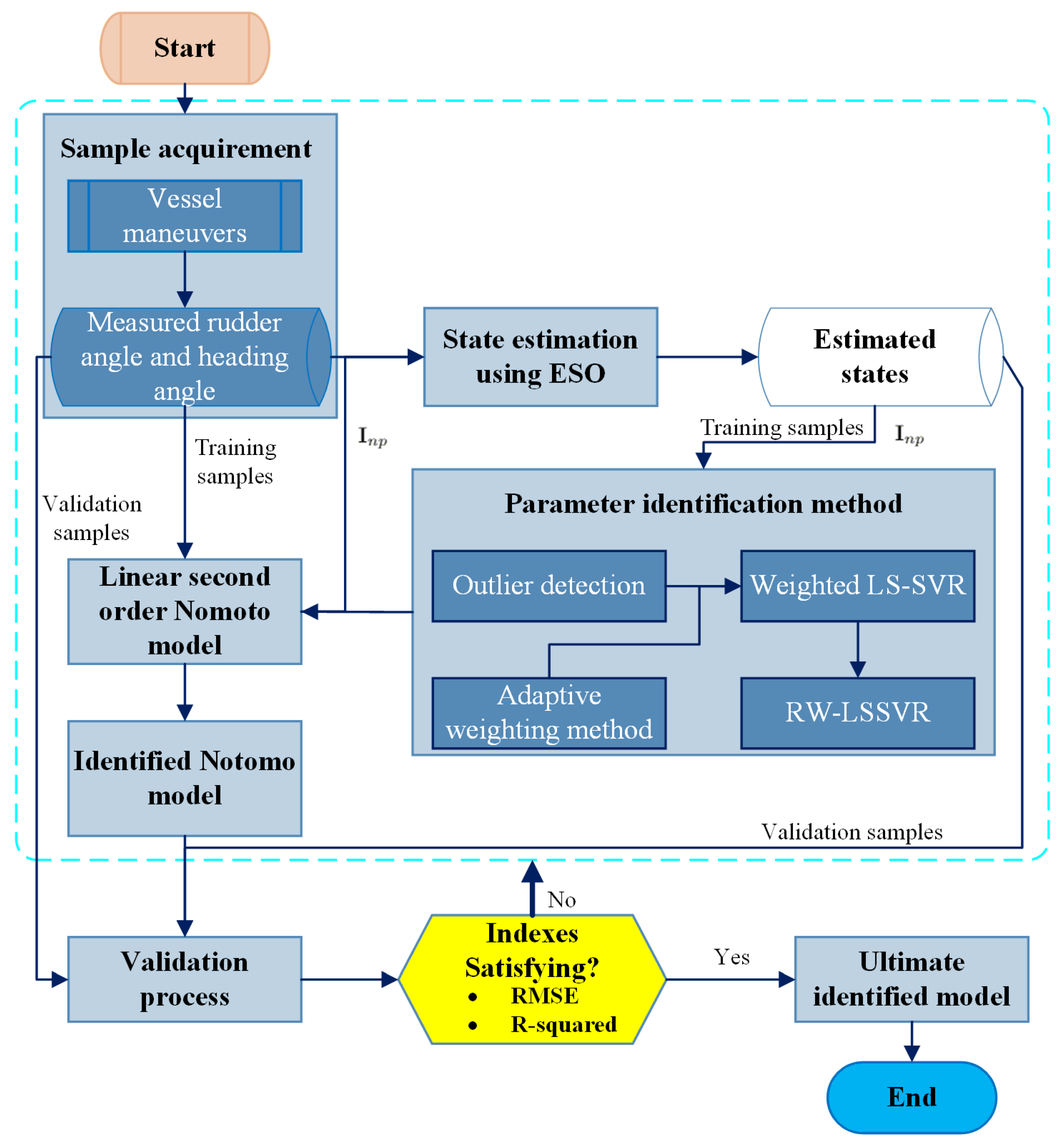
3.3. Identification Procedure

Taking the above-developed state estimation method and parameter identification approach into consideration with the objective of identifying the linear response model for autonomous vessels with high accuracy, the complete identification procedure depicted in Figure 2 is described in detail as follows.

Step 1: Sample acquirement. Several sets of autonomous vessel maneuvers are simulated to provide informative data which are further used as samples for identification. According to the practical situation and commonly available sensors, we assume that the heading angle $\psi$ and rudder angle ${\delta }_R$ could be collected directly in the experiments carried out with autonomous vessels but the rest items of input vector ${\mathbf{I}}_{np}$ are immeasurable and are required to be estimated through Step 2. A time series of samples including ${\delta }_R$ and $\psi$ is acquired with the time interval $\Delta t$ which is mainly determined by the minimum sampling frequency between the compass and the rudder sensor.

Step 2: State estimation. Estimate the immeasurable states in ${\mathbf{I}}_{np}$ including $\ddot{\psi },\dot{\psi },{\psi }^3$, ${\dot{\delta }}_R$ by using the ESO method, mainly in Equation (9) based on linear response model of autonomous vessels in Equation (4). According to the stability analysis results, the coefficients containing $l_1,l_2,l_4,l_5$ should be positive real numbers. However, there is no strict restriction on the value of $l_3$. These coefficients will be valued in the following case studies.

Step 3: Parameter identification. Samples acquired in Step 1 and the states estimated through Step 2 are divided into two groups. The first $60\%$ samples are extracted and prepared as a training data group for identifying the linear response model based on the RW-LSSVR. The remaining samples are regarded as a validation data group which is used to validate the generalization ability of the identified response model. The training data are processed by following the outlier detection procedure with three sequential steps to mitigate the outlier effects. Afterward, the preprocessed training data are transformed into the weighted LS-SVR and the nonlinear response model. The unknown parameters involved in the parameter vector $\theta$ are able to be calculated via Equation (31). Then the identified linear response model for autonomous vessels is obtained.

Step 4: Validation process. After acquiring the identified linear response model with the use of training data, it is essential to validate the generalization ability of the identified model with the objective to indicate whether its application with validation data can also produce satisfying predictions, i.e., with a small RMSE (means the error between predictions and corresponding original item) and large $R^2$. The smaller the RMSE is, the more accurate the identified model is. Meanwhile, the bigger the $R^2$ is, the more similar the trend of predictions to the corresponding original item is. If the predictions satisfy the expected standard, the ultimate identified linear response model is obtained. Otherwise, one should move back to optimize and repeat the previous three steps from Step 1 to Step 3 until reaching the ultimate identified model.

Based on the prediction ${\widehat{y}}_i$ and the desirable output $y_i$ with the total number of $n_{val}$, the calculation of RMSE and $R^2$ can be described as follows, respectively.

$${\displaystyle \mathrm{RMSE}=\sqrt{\frac{1}{n_{val}}\sum _{i=1}^{n_{val}}{\left(y_i-{\widehat{y}}_i\right)}^2}}$$

(32)

$${\displaystyle R^2=1-\frac{{\sum }_{i=1}^{n_{val}}{\left(y_i-{\widehat{y}}_i\right)}^2}{{\sum }_{i=1}^{n_{val}}{\left({\displaystyle y_i-\frac{{\sum }_{i=1}^{n_{val}}{y}_i}{n_{val}}}\right)}^2}}$$

(33)

4. Results

A case study is carried out to demonstrate the effectiveness of the ESO-based state estimation and RW-LSSVR-based parameter identification approach. Two sets of simulations are conducted. One set is used for approach verification, and the other is used to validate the generalization ability of the identified model. Simulations are implemented on the MATLAB software platform.

4.1. Experiment Setup

A linear second-order Nomoto model with predefined parameter values (listed in

Table 3. Settings of the experimental test.

Different	Cargo	Patrol	Same	Cargo	Patrol
$T_1$ (s)	45.0	2.0875	$l_1$	180
$T_2$ (s)	6.0	0.3179	$l_2$	12,150
$T_3$ (s)	10.0	0.1830	$l_3$	100
$K_R$ ($s^{-1}$)	0.09	−0.1724	$l_4$	364,500
$T_m$ (s)	5	1	$l_5$	4,100,625
$k_p$	0.12	0.7	Employed bees	30
Simulation Time (s)	6000	900	Onlooker bees	30
Total Samples	300,000	45,000	Sources	30
			$Limit$	35
			Max iteration	30
			Number of parameters	1
			Search domain	$[{10}^{-2},{10}^{10}]$
			$\Delta t$	0.02 s

) of a cargo vessel in [48] is applied for simulation tests on the proposed hybrid identification framework. In order to fully test the performance of the proposed identification approach, another relatively small vessel, a patrol river vessel, is selected as the research object [49]. All necessary settings for these two vessels are listed in Table 3, where the first column means the different settings for two vessels while the fourth column presents the same.

$\Delta t$ is set under the consideration of minimum logging interval between practical compass for measuring heading angle and rudder sensor for rudder angle. Considering that the goal of this study is to evaluate the effectiveness of the proposed hybrid identification approach incorporating the ESO-based state estimator with the RW-LSSVR identification method, the maximum informative excitation of the input signal is referred to as the widely used sinusoidal excitation signal which to high degrees matches the requirement of unbiased identification of the system parameters [42]. The initial heading angle and rudder angle are zero, respectively.

The observer gains of the ESO are set according to the comprehensive analysis and experimental results from validating ESO performance in [50], especially regarding the impacts of the observer bandwidths on estimation results and sensitivity to noises. For the purpose of good demonstration, the ESO is compared with the EKF on the state estimate. Moreover, in order to well investigate the effectiveness and robustness of the proposed hybrid identification approach, the data is noised by corrupted with the simulated disturbances using a Gaussian distribution.

One issue regarding the RW-LSSVR identification method is the particular setting for the regularization parameter which is handled by the artificial bee colony algorithm (ABC) referred to in our previous work in [6]. The ABC is initialized as Table 3 shown. To well present the performance of the identification method, the LS-SVR method is selected for comparison, and its parameters are also optimized by the ABC algorithm with the same initial settings.

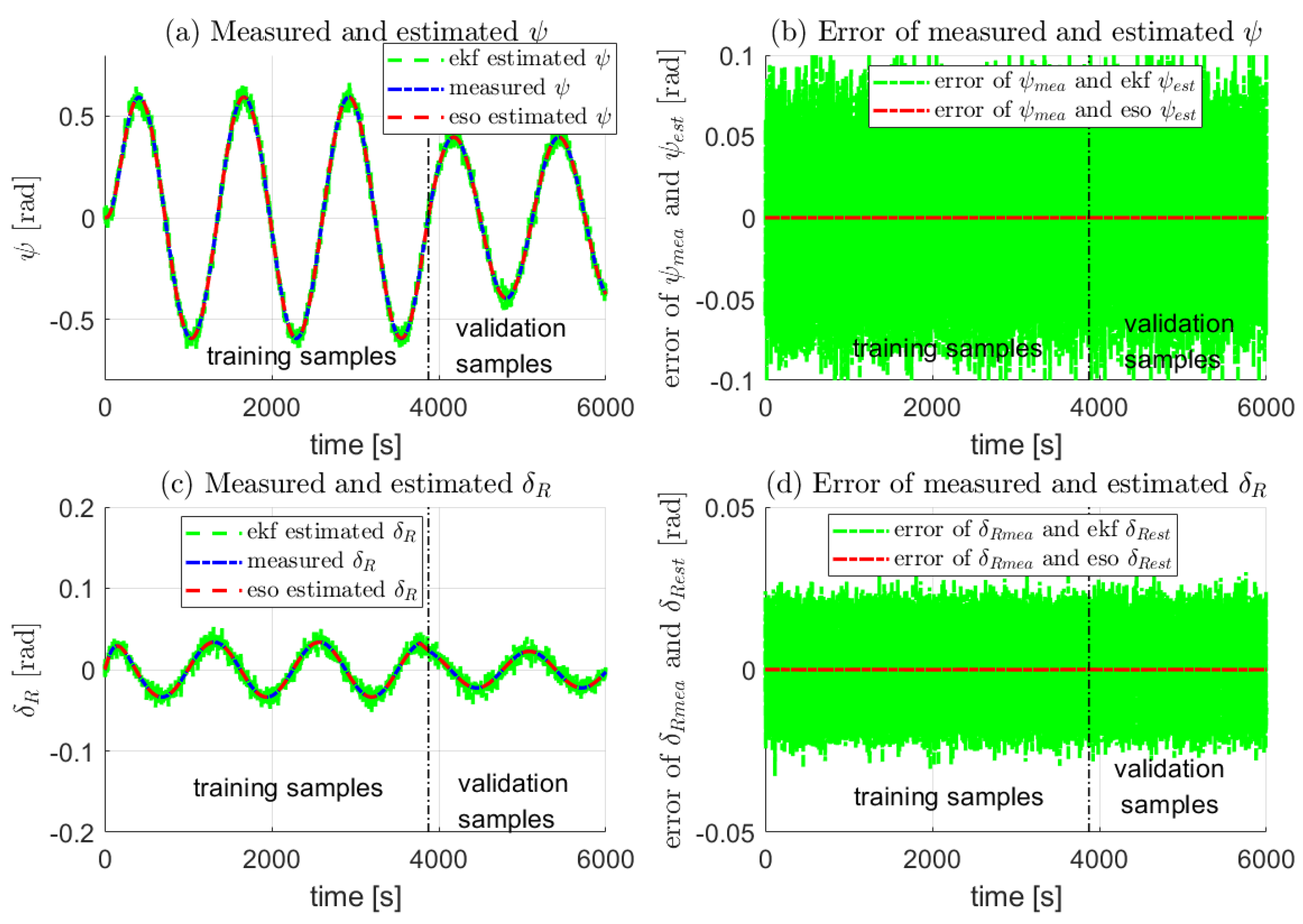
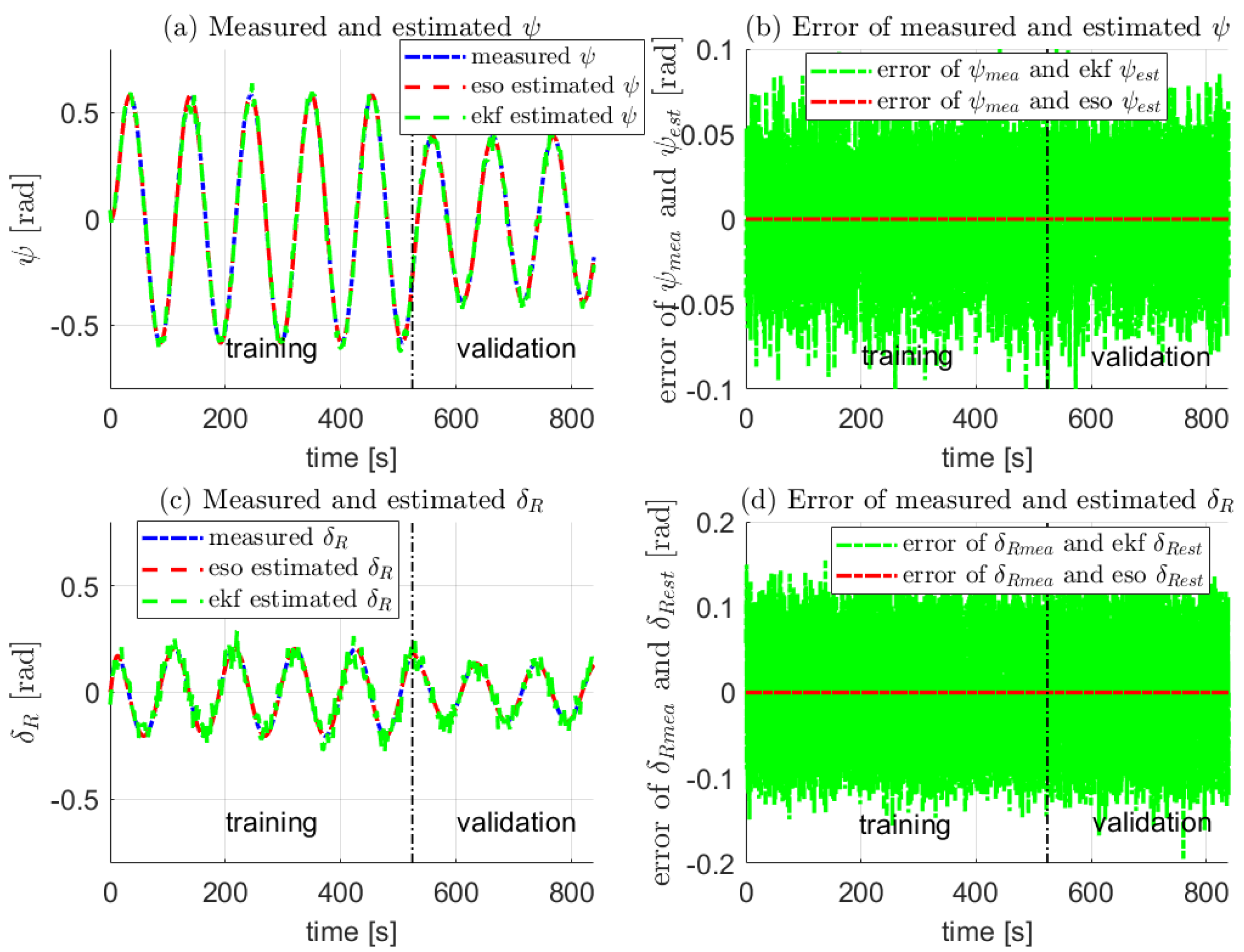
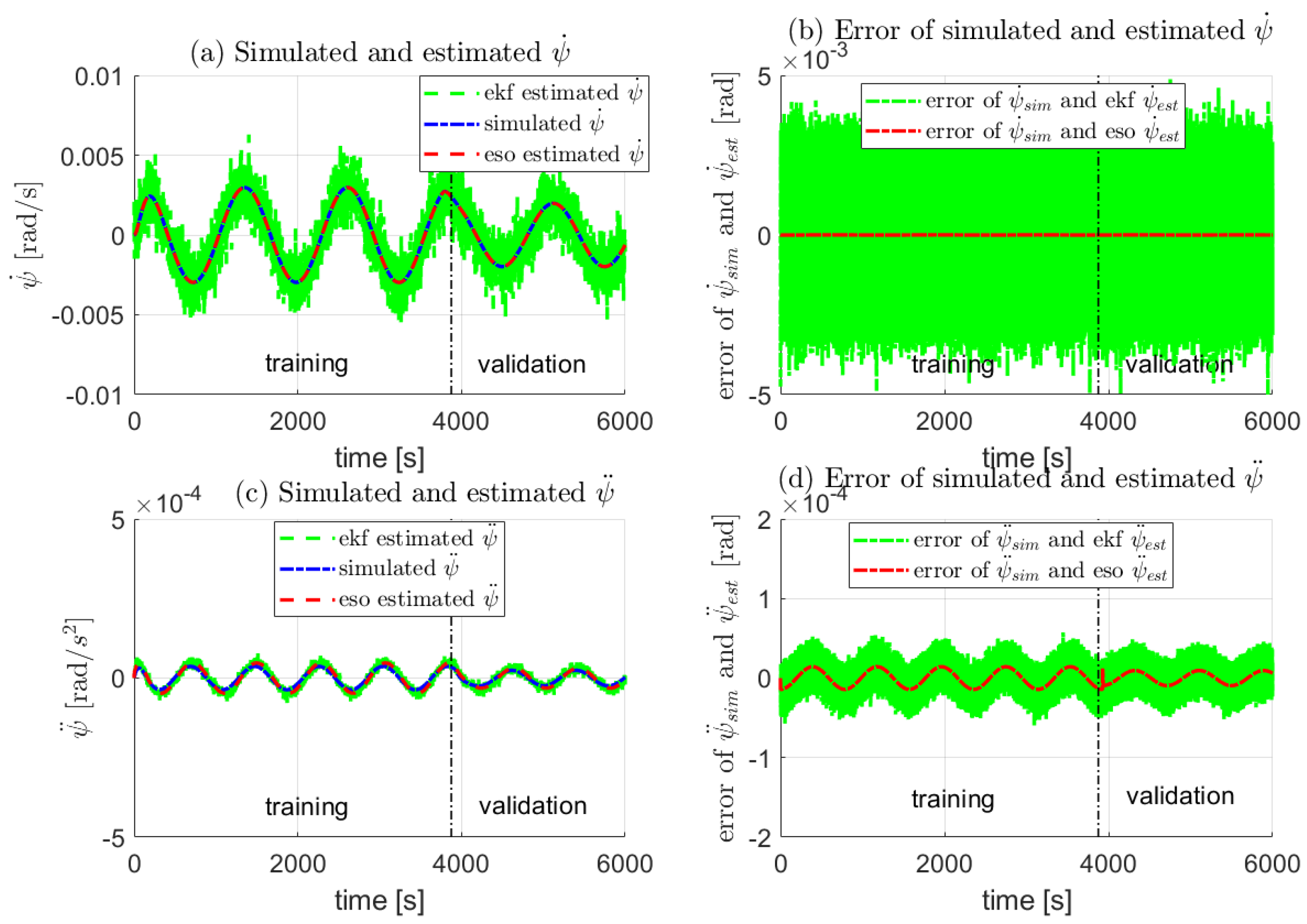
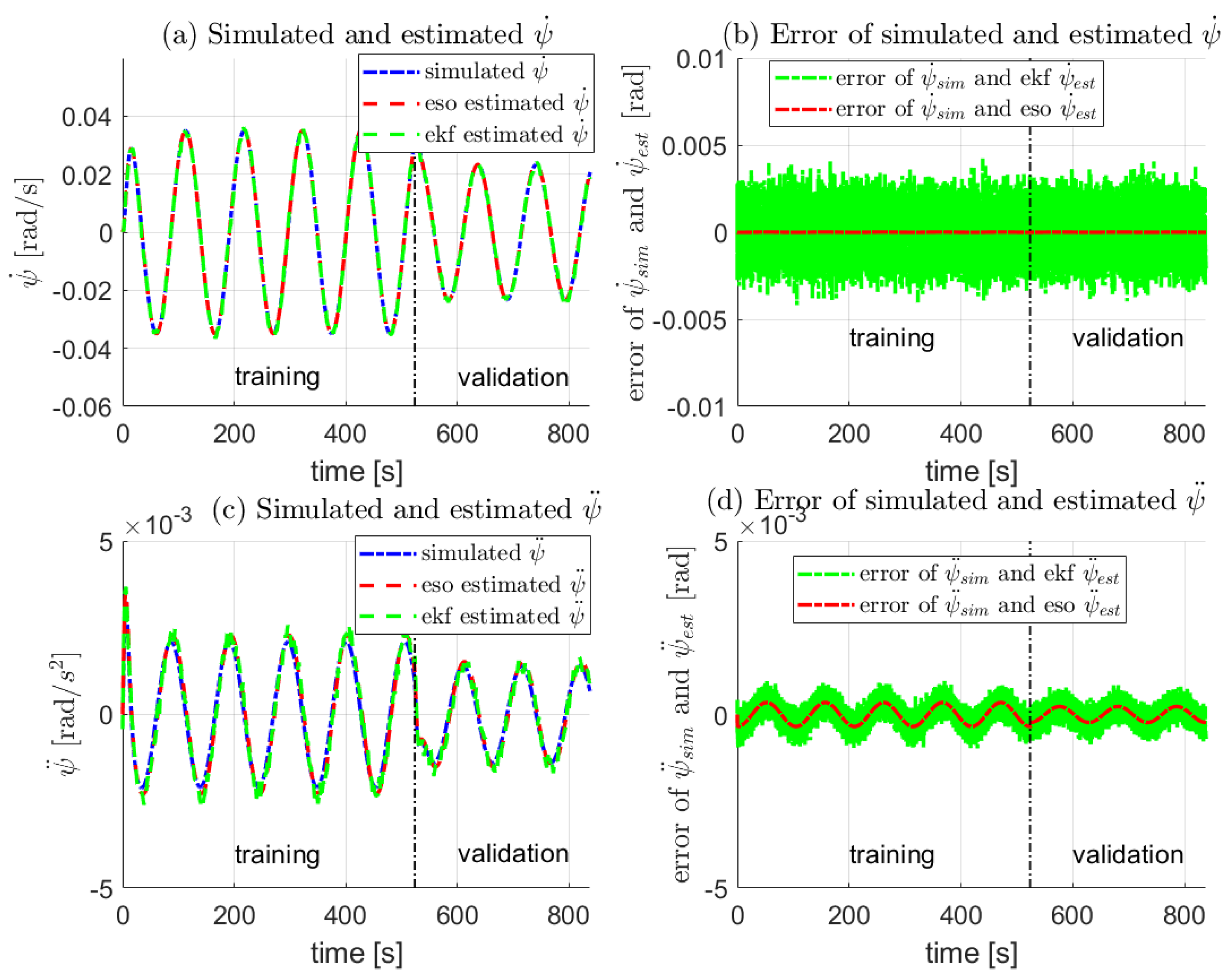
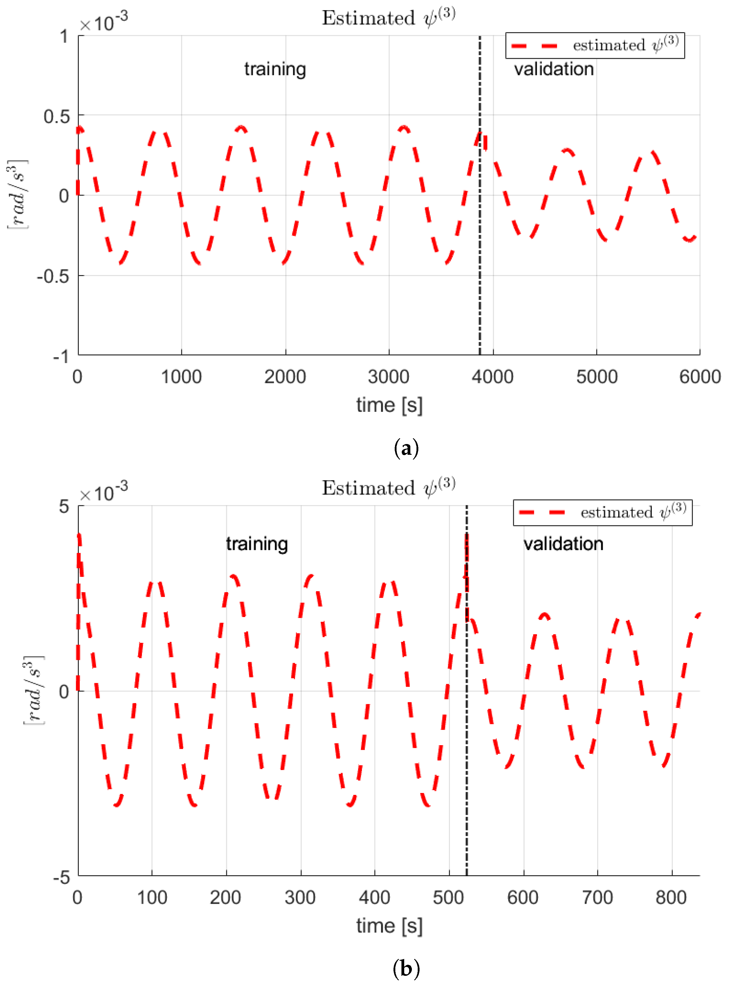
4.2. State Estimation Results

The measurements including the heading angle and the rudder angle are given in Figure 3 for the cargo vessel and Figure 4 for the patrol vessel where the estimations are also plotted for comparative analysis. Figure 5 and Figure 6 show the estimates and observer errors for both vessels, respectively. The simulated samples presenting immeasurable states are also shown. The errors of estimates and measurements or simulated states in terms of RMSE and $R^2$ are listed in

Table 4. Error of estimations and measurements or simulations for vessels.

Index	State	ESO		EKF
		Cargo	Patrol	Cargo	Patrol
RMSE	$\psi \left(rad\right)$	$2.3045\times {10}^{-15}$	$2.0021\times {10}^{-14}$	$8.9993\times {10}^{-9}$	$9.6531\times {10}^{-9}$
	$\dot{\psi }\left(rad/s\right)$	$2.3045\times {10}^{-11}$	$5.0013\times {10}^{-10}$	$9.9977\times {10}^{-8}$	$8.4211\times {10}^{-7}$
	$\ddot{\psi }\left(rad/s^2\right)$	$3.2407\times {10}^{-8}$	$7.324\times {10}^{-8}$	$6.4298\times {10}^{-8}$	$7.0672\times {10}^{-8}$
	${\delta }_R\left(rad\right)$	$2.3266\times {10}^{-11}$	$5.2236\times {10}^{-11}$	$1.7822\times {10}^{-8}$	$2.3266\times {10}^{-8}$
	$\stackrel{⃛}{\psi }\left(rad/s^3\right)$	-	-	-	-
$R^2$	$\psi$	1.0000	1.0000	0.9902	0.9953
	$\dot{\psi }$	0.9999	1.0000	0.9970	9010
	$\stackrel{⃛}{\psi }$	0.9732	0.9651	0.9469	0.9341
	${\delta }_R$	1.0000	1.0000	0.8919	0.8557
	$\stackrel{⃛}{\psi }$	-	-	-	-

. From the estimation results, it can be found that the RMSEs of ESO and EKF are both close to zero. The RMSEs of states from the ESO for the cargo vessel are smaller than those for the patrol vessel. Comparatively, the RMSEs of the ESO for both vessels are smaller than these of the EKF. The $R^2$s of $\psi$, $\dot{\psi }$, ${\delta }_R$ related to the ESO for the patrol vessel are 1 except for that of $\ddot{\psi }$. For the cargo vessel, the $R^2$s of $\psi$ and ${\delta }_R$ from the ESO are 1. The $R^2$s of the left states estimated by the ESO are not 1 but the trend of the estimated and simulated of each of them is still very similar. The $R^2$s of all states estimated by the EKF are less than 1. What is more, the $R^2$ of each state estimated by the EKF is smaller than the corresponding one estimated by the ESO. Therefore, it can be revealed that the ESO shows superior performance on the state estimate over the EKF. Estimate results of the ESO are selected to be used in the following identification procedure.

Notice that the $R^2$ of $\ddot{\psi }$ for the cargo vessel is a little smaller than that for the patrol vessel due to the larger inertia of the former vessel making a relatively slower reaction. Following the above calculation and the selections of state estimates from the ESO, i.e., $x_5=\dot{x_4}+u$, the estimates of $\stackrel{⃛}{\psi }$ of the two vessels are plotted in Figure 7. The estimation results imply that high-accuracy estimates are able to be utilized in the upcoming parameter identification process. It is noticeable that the sampling frequency is found to be influential on the estimation results of the ESO. If a very low sampling frequency is used, important information may be missing in the measurement and cause inaccurate state estimation, resulting in a poorly identified model. This should be considered in the process of selecting suitable sensors.

4.3. Identification Results

Following the identification procedure in Section 3.3, the identified parameters of the linear response model for the cargo vessel are listed in

Table 5. Identification results of the linear response model for vessels.

Parameter	Nominal		Identified (RW-LSSVR)		Identified (LSSVR)		Relative Error (%) (RW-LSSVR)		Relative Error (%) (LSSVR)
	Cargo	Patrol	Cargo	Patrol	Cargo	Patrol	Cargo	Patrol	Cargo	Patrol
$T_1$ (s)	45	2.0875	46.21	2.0896	46.93	2.0231	2.689	0.1006	4.289	−3.085
$T_2$ (s)	6.0	0.3179	5.960	0.3035	6.09	0.297	−0.6667	−4.530	1.5	−6.574
$T_3$ (s)	10	0.1830	9.751	0.1840	9.932	0.1921	−2.49	0.5464	−0.68	4.973
$K_R$ ($s^{-1}$)	0.090	−0.1724	0.095	−0.1837	0.087	−0.189	5.23	6.4721	−3.333	9.629

. The nominal values of parameters are presented for comparative purposes. To quantitatively indicate the identification errors, the relative error for each parameter is calculated by the ratio of error between the identified and nominal values. It can be observed from the identification results in terms of the relative errors of both identification methods i.e., RW-LSSVR and LS-SVR are very small, which implies the identified model is of high accuracy. Comparatively, the relative errors of the RW-LSSVR are smaller than these of the LS-SVR. So it can be concluded that the model identified by the RW-LSSVR is much more accurate than that by the LS-SVR. This is due to the robust ability of the RW-LSSVR on noise detection and filter.

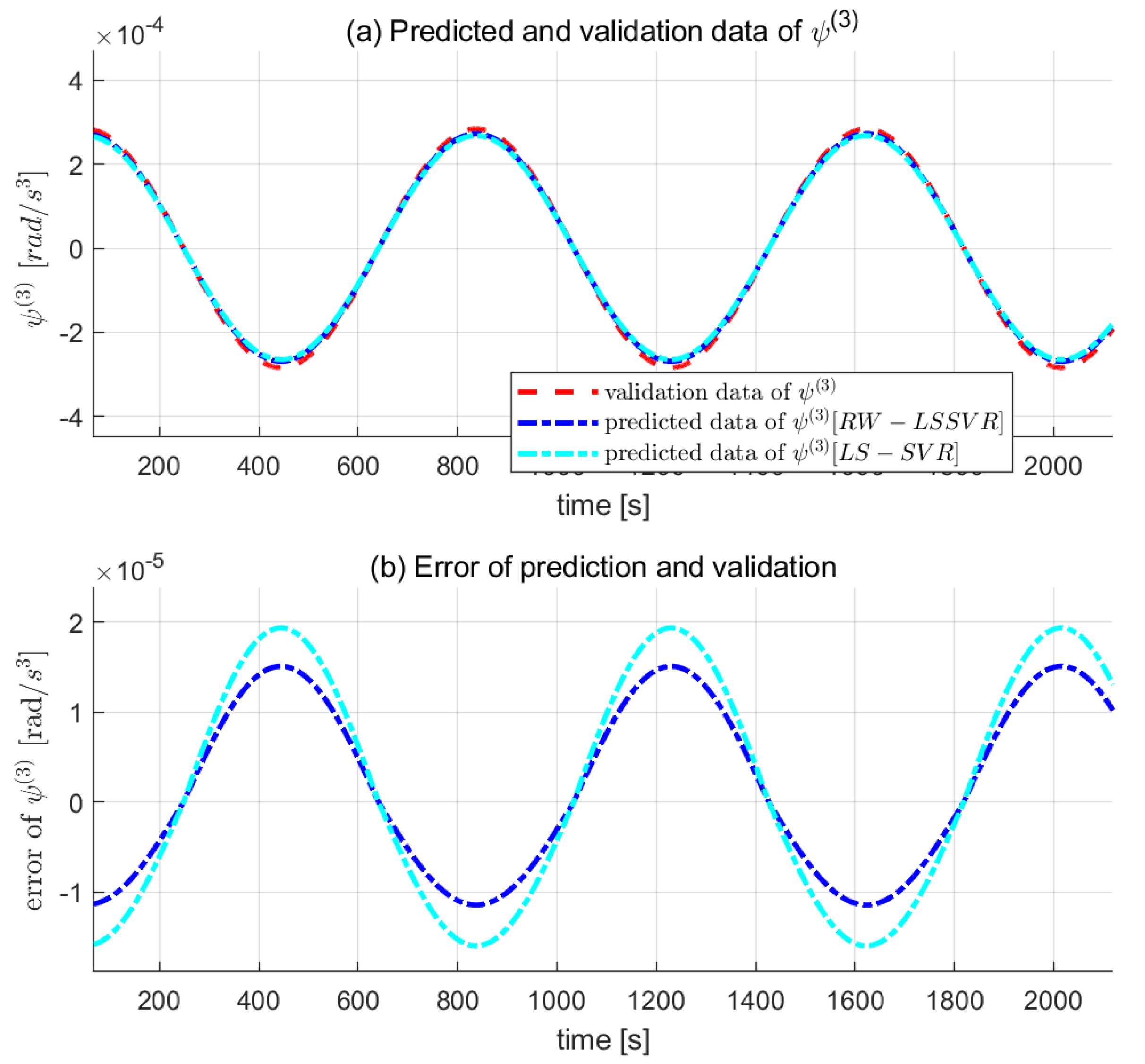
4.4. Validation of the Identified Model

The prediction results of the identified response models with the use of validation samples are shown in Figure 8 for the cargo vessel and Figure 9 for the patrol vessel. The prediction errors in terms of RMSE and $R^2$ are given in

Table 6. Prediction errors of the identified linear steering model for the two vessels.

Index	RW-LSSVR		LSSVR
	Cargo	Patrol	Cargo	Patrol
$\mathrm{RMSE}$ ($\times {10}^{-11}$, rad/s${}^3$)	9.9232	544.53	17.454	789.04
$R^2$	0.9978	0.9974	0.9961	0.9963

. It can be seen from the prediction results that the predictions from the identified model by the RW-LSSVR much better track the validation samples with relatively high accuracy compared with that of the LS-SVR. Therefore, the performance of our proposed identification approach in identifying the linear response model is effectively proved to be satisfactory through the simulation study on a cargo vessel as well as a patrol vessel.

5. Conclusions and Future Work

5.1. Conclusions

In this section, a summary of the research findings of the investigation is presented. This paper developed a hybrid framework for autonomous vessel linear response model identification based on the estimated states using the ESO method. The concrete and logically ordered work on dynamic model parameters identification for autonomous vessels is a step toward successful implementation of the mathematical dynamic model to describe vessel dynamic characteristics and support the model application requirements of vessel control system design.

In the process of parameter identification investigation, the practical situation with only compass and rudder angle sensors being available is considered. Two vessels using linear response models with predefined parameters are employed to generate simulated data for validation of the proposed hybrid identification approach. Based on the directly measured heading angle and rudder angle, the immeasurable states can be estimated with almost negligible deviation by the ESO method, mainly due to parts of the model information being known. It is noticeable that the ESO method outperforms the EKF on immeasurable state estimation in terms of computational cost and estimation errors. Furthermore, the RW-LSSVR identification method extracted from our previous study [6] also indicates good identification performance when compared with the typical identification method, i.e., LS-SVR.

Unlike the commonly investigated identification-based modeling of vessel dynamics where the immeasurable states are seldom discussed, the proposed hybrid identification approach has simultaneously paid attention to the immeasurable state estimation and vessel dynamic model identification. From the research findings of this work, it can be concluded that the proposed hybrid identification approach is a novel inspiration and a new solution for the development of identification-based modeling of vessel dynamics based on the proven effectiveness and attractive advantages of the approach. In addition, the approach is relatively “cheap” due to only some data being logged by generally low-cost sensors being required to feed into the approach, which in turn shows its good potential applications in shipping.

5.2. Future Work

On the basis of the current findings, several aspects can be future explored to enhance the performance and applications of the proposed hybrid identification approach for future work. Three main aspects are listed as follows:

• Optimize the hybrid identification approach. Although the proposed identification method has achieved good estimation and identification results, there are some points that deserved to be addressed for the hyper-parameters in the RW-LSSVR, such as initial weight and penalty factor significantly impacting the identification performance. These hyper-parameters are required to be effectively set, which can be regarded as an optimization problem. Apart from the ABC algorithm used in this work, many new algorithms can be alternatives, such as the partially coupled nonlinear parameter optimization algorithm [51], the metaheuristic approach [52], the prairie dog optimization algorithm [53], the deep learning algorithm [54], and so on. It is a new attempt to apply these algorithms to improve identification performance.
• Expend the scope of evaluation scenarios. In this study, one degree of freedom (DOF) dynamic concerning the heading response was modeled based on the hybrid identification approach. The proposed approach can be extended to other kinds of autonomous vessel dynamic models such as the 3 DOF horizontal model, and 4 DOF dynamic model. Satisfactory evaluation of the proposed hybrid identification approach comes from the simulation study as well as the field experimental study. In future research, efforts should be made to carry out experimental studies on the proposed approach as well as to improve the identification accuracy. Moreover, the impacts induced by noisy measurements involving real environmental disturbances and sensor noises will be further studied.
• Modify the approach to be applicable to online identification. The hybrid identification approach was proposed mainly for offline identification of the response models for two autonomous vessels respectively. In the future, more complicated situations can be considered. According to the Froude number [7,55], vessel motion mode is varied along with the changes in the vessel speed or the loading condition. Interests in how these two factors affect vessel motions have been paid with the use of online identification methods [56,57]. From recent research on SVM issues, the SVM-based identification method was modified into an online version, e.g., the multi-innovation gradient SVM studied in [58]. Similarly, the upcoming research point on the proposed hybrid identification approach could be a suitable modification to make the approach an online one.

References

1. Munim, Z.H. Autonomous ships: A review, innovative applications and future maritime business models. In Supply Chain Forum: An International Journal; Taylor & Francis: Abingdon, UK, 2019; Volume 20, pp. 266–279. [Google Scholar]
2. Rødseth, Ø.J. From concept to reality: Unmanned merchant ship research in Norway. In Proceedings of the Underwater Technology (UT), Busan, Korea, 21–24 February 2017. [Google Scholar]
3. Wróbel, K.; Montewka, J.; Kujala, P. Towards the assessment of potential impact of unmanned vessels on maritime transportation safety. Reliab. Eng. Syst. Saf. 2017, 165, 155–169. [Google Scholar] [CrossRef]
4. Gu, Y.; Goez, J.C.; Guajardo, M.; Wallace, S.W. Autonomous vessels: State of the art and potential opportunities in logistics. Int. Trans. Oper. Res. 2019, 28, 1706–1739. [Google Scholar] [CrossRef]
5. Fossen, T.I. Handbook of Marine Craft Hydrodynamics and Motion Control; John Wiley & Sons: Hoboken, NJ, USA, 2011. [Google Scholar]
6. Zhu, M.; Sun, W.; Hahn, A.; Wen, Y.; Xiao, C.; Tao, W. Adaptive modeling of maritime autonomous surface ships with uncertainty using a weighted LS-SVR robust to outliers. Ocean. Eng. 2020, 200, 107053. [Google Scholar] [CrossRef]
7. Zhu, M. Optimized Support Vector Regression Algorithm-Based Modeling of Ship Dynamics. Ph.D. Thesis, Universität Oldenburg, Oldenburg, Germany, 2018. [Google Scholar]
8. Liu, C.; Negenborn, R.R.; Zheng, H.; Chu, X. A state-compensation extended state observer for model predictive control. Eur. J. Control 2017, 36, 1–9. [Google Scholar] [CrossRef]
9. Guo, H.p.; Zou, Z.j. System-based investigation on 4-DOF ship maneuvering with hydrodynamic derivatives determined by RANS simulation of captive model tests. Appl. Ocean. Res. 2017, 68, 11–25. [Google Scholar] [CrossRef]
10. Wang, Z.; Xu, H.; Xia, L.; Zou, Z.; Soares, C.G. Kernel-based support vector regression for nonparametric modeling of ship maneuvering motion. Ocean. Eng. 2020, 216, 107994. [Google Scholar] [CrossRef]
11. Prpić-Oršić, J.; Valčić, M.; Čarija, Z. A Hybrid Wind Load Estimation Method for Container Ship Based on Computational Fluid Dynamics and Neural Networks. J. Mar. Sci. Eng. 2020, 8, 539. [Google Scholar] [CrossRef]
12. Du, P.; Cheng, L.; Tang, Z.j.; Ouahsine, A.; Hu, H.b.; Hoarau, Y. Ship maneuvering prediction based on virtual captive model test and system dynamics approaches. J. Hydrodyn. 2022, 34, 259–276. [Google Scholar] [CrossRef]
13. Andersson, J.; Shiri, A.A.; Bensow, R.E.; Yixing, J.; Chengsheng, W.; Gengyao, Q.; Deng, G.; Queutey, P.; Xing-Kaeding, Y.; Horn, P.; et al. Ship-scale CFD benchmark study of a pre-swirl duct on KVLCC2. Appl. Ocean. Res. 2022, 123, 103134. [Google Scholar] [CrossRef]
14. Ljung, L. Perspectives on system identification. Annu. Rev. Control 2010, 34, 1–12. [Google Scholar] [CrossRef] [Green Version]
15. Gevers, M. A personal view of the development of system identification: A 30-year journey through an exciting field. IEEE Control Syst. Mag. 2006, 26, 93–105. [Google Scholar]
16. Wang, Z.; Soares, C.G.; Zou, Z. Optimal design of excitation signal for identification of nonlinear ship manoeuvring model. Ocean Eng. 2020, 196, 106778. [Google Scholar] [CrossRef]
17. Meng, Y.; Zhang, X.; Zhu, J. Parameter identification of ship motion mathematical model based on full-scale trial data. Int. J. Nav. Archit. Ocean. Eng. 2022, 14, 100437. [Google Scholar] [CrossRef]
18. Guan, W.; Peng, H.; Zhang, X.; Sun, H. Ship Steering Adaptive CGS Control Based on EKF Identification Method. J. Mar. Sci. Eng. 2022, 10, 294. [Google Scholar] [CrossRef]
19. Zhang, X.; Meng, Y.; Liu, Z.; Zhu, J. Modified grey wolf optimizer-based support vector regression for ship maneuvering identification with full-scale trial. J. Mar. Sci. Technol. 2022, 27, 576–588. [Google Scholar] [CrossRef]
20. Xue, Y.; Liu, Y.; Ji, C.; Xue, G.; Huang, S. System identification of ship dynamic model based on Gaussian process regression with input noise. Ocean Eng. 2020, 216, 107862. [Google Scholar] [CrossRef]
21. Wang, L.; Li, S.; Liu, J.; Wu, Q. Data-driven model identification and predictive control for path-following of underactuated ships with unknown dynamics. Int. J. Nav. Archit. Ocean Eng. 2022, 14, 100445. [Google Scholar] [CrossRef]
22. Miyauchi, Y.; Maki, A.; Umeda, N.; Rachman, D.M.; Akimoto, Y. System parameter exploration of ship maneuvering model for automatic docking/berthing using CMA-ES. J. Mar. Sci. Technol. 2022, 27, 1065–1083. [Google Scholar] [CrossRef]
23. Song, C.; Zhang, X.; Zhang, G. Nonlinear identification for 4-DOF ship maneuvering modeling via full-scale trial data. IEEE Trans. Ind. Electron. 2021, 69, 1829–1835. [Google Scholar] [CrossRef]
24. Chen, C.; Ruiz, M.T.; Delefortrie, G.; Mei, T.; Vantorre, M.; Lataire, E. Parameter estimation for a ship’s roll response model in shallow water using an intelligent machine learning method. Ocean Eng. 2019, 191, 106479. [Google Scholar] [CrossRef]
25. Wang, Z.; Zou, Z.; Soares, C.G. Identification of ship manoeuvring motion based on nu-support vector machine. Ocean Eng. 2019, 183, 270–281. [Google Scholar] [CrossRef]
26. Simpkins, A. System identification: Theory for the user, (ljung, l.; 1999) [on the shelf]. IEEE Robot. Autom. Mag. 2012, 19, 95–96. [Google Scholar] [CrossRef]
27. Schoukens, J.; Ljung, L. Nonlinear system identification: A user-oriented road map. IEEE Control Syst. Mag. 2019, 39, 28–99. [Google Scholar] [CrossRef]
28. Han, J. From PID to active disturbance rejection control. IEEE Trans. Ind. Electron. 2009, 56, 900–906. [Google Scholar] [CrossRef]
29. Liu, J.; Vazquez, S.; Wu, L.; Marquez, A.; Gao, H.; Franquelo, L.G. Extended state observer-based sliding-mode control for three-phase power converters. IEEE Trans. Ind. Electron. 2016, 64, 22–31. [Google Scholar] [CrossRef]
30. Stanković, M.R.; Rapaić, M.R.; Manojlović, S.M.; Mitrović, S.T.; Simić, S.M.; Naumović, M.B. Optimised active disturbance rejection motion control with resonant extended state observer. Int. J. Control 2019, 92, 1815–1826. [Google Scholar] [CrossRef]
31. Sun, T.; Zhang, J.; Pan, Y. Active disturbance rejection control of surface vessels using composite error updated extended state observer. Asian J. Control 2017, 19, 1802–1811. [Google Scholar] [CrossRef]
32. Shi, D.; Wu, Z.; Chou, W. Anti-disturbance trajectory tracking of quadrotor vehicles via generalized extended state observer. J. Vib. Control 2020, 26, 1173–1186. [Google Scholar] [CrossRef]
33. Liu, Z.; Wang, Y.; Liu, S.; Li, Z.; Zhang, H.; Zhang, Z. An approach to suppress low-frequency oscillation by combining extended state observer with model predictive control of EMUs rectifier. IEEE Trans. Power Electron. 2019, 34, 10282–10297. [Google Scholar] [CrossRef]
34. Luenberger, D. An introduction to observers. IEEE Trans. Autom. Control 1971, 16, 596–602. [Google Scholar] [CrossRef]
35. Gu, D.K.; Liu, Q.Z.; Liu, Y.D. Parametric design of functional interval observer for time-delay systems with additive disturbances. Circuits Syst. Signal Process. 2022, 41, 2614–2635. [Google Scholar] [CrossRef]
36. Li, S.; Yan, Y.; Jiang, D.; Guo, Q. Synchronized control of multiple electrohydraulic systems with terminal sliding mode observer under parametric uncertainty and external load. ISA Trans. 2022. [Google Scholar] [CrossRef] [PubMed]
37. Deng, C.; Wen, C.; Huang, J.; Zhang, X.M.; Zou, Y. Distributed observer-based cooperative control approach for uncertain nonlinear MASs under event-triggered communication. IEEE Trans. Autom. Control 2021, 67, 2669–2676. [Google Scholar] [CrossRef]
38. Liu, J.; Shen, X.; Alcaide, A.M.; Yin, Y.; Leon, J.I.; Vazquez, S.; Wu, L.; Franquelo, L.G. Sliding Mode Control of Grid-Connected Neutral-Point-Clamped Converters Via High-Gain Observer. IEEE Trans. Ind. Electron. 2022, 69, 4010–4021. [Google Scholar] [CrossRef]
39. Tong, S.; Min, X.; Li, Y. Observer-based adaptive fuzzy tracking control for strict-feedback nonlinear systems with unknown control gain functions. IEEE Trans. Cybern. 2020, 50, 3903–3913. [Google Scholar] [CrossRef] [PubMed]
40. Moradi, E.; Mohseni, R. Parameters estimation of linear frequency modulated signal using Kalman filter and its extended versions. Signal Image Video Process. 2022, 1–9. [Google Scholar] [CrossRef]
41. Banazadeh, A.; Ghorbani, M. Frequency domain identification of the Nomoto model to facilitate Kalman filter estimation and PID heading control of a patrol vessel. Ocean Eng. 2013, 72, 344–355. [Google Scholar] [CrossRef]
42. Perera, L.P.; Oliveira, P.; Soares, C.G. System identification of vessel steering with unstructured uncertainties by persistent excitation maneuvers. IEEE J. Ocean. Eng. 2015, 41, 515–528. [Google Scholar] [CrossRef]
43. Erazo, C.; Angulo, F.; Olivar, G. Stability analysis of the extended state observers by Popov criterion. Theor. Appl. Mech. Lett. 2012, 2, 043006. [Google Scholar] [CrossRef]
44. Shahsavar, A.; Bagherzadeh, S.A.; Mahmoudi, B.; Hajizadeh, A.; Afrand, M.; Nguyen, T.K. Robust Weighted Least Squares Support Vector Regression algorithm to estimate the nanofluid thermal properties of water/graphene Oxide–Silicon carbide mixture. Phys. A Stat. Mech. Its Appl. 2019, 525, 1418–1428. [Google Scholar] [CrossRef]
45. Suykens, J.A.; De Brabanter, J.; Lukas, L.; Vandewalle, J. Weighted least squares support vector machines: Robustness and sparse approximation. Neurocomputing 2002, 48, 85–105. [Google Scholar] [CrossRef]
46. Pearson, R.K. Outliers in process modeling and identification. IEEE Trans. Control Syst. Technol. 2002, 10, 55–63. [Google Scholar] [CrossRef]
47. De Brabanter, K. Least Squares Support Vector Regression with Applications to Large-Scale Data: A Statistical Approach; Faculty of Engineering, KU Leuven, Katholieke Universiteit Leuven: Leuven, Belgium, 2011. [Google Scholar]
48. Nomoto, K.; Taguchi, K. On steering qualities of ships (2). J. Zosen Kiokai 1957, 1957, 57–66. [Google Scholar] [CrossRef]
49. Carrillo, S.; Contreras, J. Obtaining First and Second Order Nomoto Models of a Fluvial Support Patrol using Identification Techniques. Ship Sci. Technol. 2018, 11, 19–28. [Google Scholar] [CrossRef]
50. Zheng, Q.; Gao, L.Q.; Gao, Z. On validation of extended state observer through analysis and experimentation. J. Dyn. Syst. Meas. Control 2012, 134, 024505. [Google Scholar] [CrossRef]
51. Zhou, Y.; Zhang, X.; Ding, F. Partially-coupled nonlinear parameter optimization algorithm for a class of multivariate hybrid models. Appl. Math. Comput. 2022, 414, 126663. [Google Scholar] [CrossRef]
52. Li, C.; Chen, G.; Liang, G.; Luo, F.; Zhao, J.; Dong, Z.Y. Integrated optimization algorithm: A metaheuristic approach for complicated optimization. Inf. Sci. 2022, 586, 424–449. [Google Scholar] [CrossRef]
53. Ezugwu, A.E.; Agushaka, J.O.; Abualigah, L.; Mirjalili, S.; Gandomi, A.H. Prairie dog optimization algorithm. Neural Comput. Appl. 2022, 1–49. [Google Scholar] [CrossRef]
54. Lv, S.X.; Wang, L. Deep learning combined wind speed forecasting with hybrid time series decomposition and multi-objective parameter optimization. Appl. Energy 2022, 311, 118674. [Google Scholar] [CrossRef]
55. Faltinsen, O.M. Hydrodynamics of High-Speed Marine Vehicles; Cambridge University Press: Cambridge, UK, 2005. [Google Scholar]
56. Himaya, A.N.; Sano, M.; Suzuki, T.; Shirai, M.; Hirata, N.; Matsuda, A.; Yasukawa, H. Effect of the loading conditions on the maneuverability of a container ship. Ocean Eng. 2022, 247, 109964. [Google Scholar] [CrossRef]
57. Wang, S.; Wang, L.; Im, N.; Zhang, W.; Li, X. Real-time parameter identification of ship maneuvering response model based on nonlinear Gaussian Filter. Ocean Eng. 2022, 247, 110471. [Google Scholar] [CrossRef]
58. Ma, H.; Ding, F.; Wang, Y. A novel multi-innovation gradient support vector machine regression method. ISA Trans. 2022. [Google Scholar] [CrossRef] [PubMed]
Figure 1. Framework of the proposed hybrid identification approach.
Jmse 10 01291 g001
Figure 2. Identification procedure of the proposed hybrid identification approach.
Jmse 10 01291 g002
Figure 3. Measurements and estimates of heading angle ψ and rudder angle δ R of the cargo vessel. The data on the left side of the black dotted line are training samples and on the right side are validation samples.
Jmse 10 01291 g003
Figure 4. Measurements and estimates of heading angle ψ and rudder angle δ R of the patrol vessel. The data on the left side of the black dotted line are training samples and on the right side are validation samples.
Jmse 10 01291 g004
Figure 5. Estimated states of the cargo vessel. The data on the left side of the black dotted line are training samples and on the right side are validation samples.
Jmse 10 01291 g005
Figure 6. Estimated states of the patrol vessel. The data on the left side of the black dotted line are training samples and on the right side are validation samples.
Jmse 10 01291 g006
Figure 7. Estimates of ψ of the two vessels. The data on the left side of the black dotted line are training samples and on the right side are validation samples. (a) Cargo vessel. (b) Patrol vessel.
Jmse 10 01291 g007
Figure 8. Prediction results of the cargo vessel. (a) Predicted and estimated ψ ; (b) error of ψ .
Jmse 10 01291 g008
Figure 9. Prediction results of the patrol vessel. (a) Predicted and estimated ψ ; (b) error of ψ .
Jmse 10 01291 g009