
A Multidisciplinary Approach for A Better Knowledge of the Benthic Habitat and Community Distribution in the Central and Western English Channel

 , , ,
, , ,
Abstract
:1. Introduction
2. General Characteristics of the English Channel
3. Material and Methods Used during the Videocharm 2011 and 2011 Campaigns
3.1. Side Scan Sonar Observations
- Zone with ribbons;
- Zone with furrows;
- Zone with dunes: small and medium/large and very large dunes;
- Sand veneer on rocks;
- Homogeneous zone;
- Table rocks, outcropping or sub-flush rocks;
- Rocky area;
- Presence of anthropic evidence: net traces (dredge or trawl) and wreck.
3.2. Grab Sample Collection
3.3. Remotely Operated Vehicle
3.4. Database and Statistical Analyses
4. Results
4.1. Side Scan Sonar Observations
4.2. Sediment
4.3. General Patterns of the Fauna
4.4. Pattern of the 2 mm Macrofauna
4.5. Pattern of the 1 + 2 mm Macrofauna
4.6. Pattern of the 1 + 2 mm Macrofauna + Colonial Epifauna Taxa
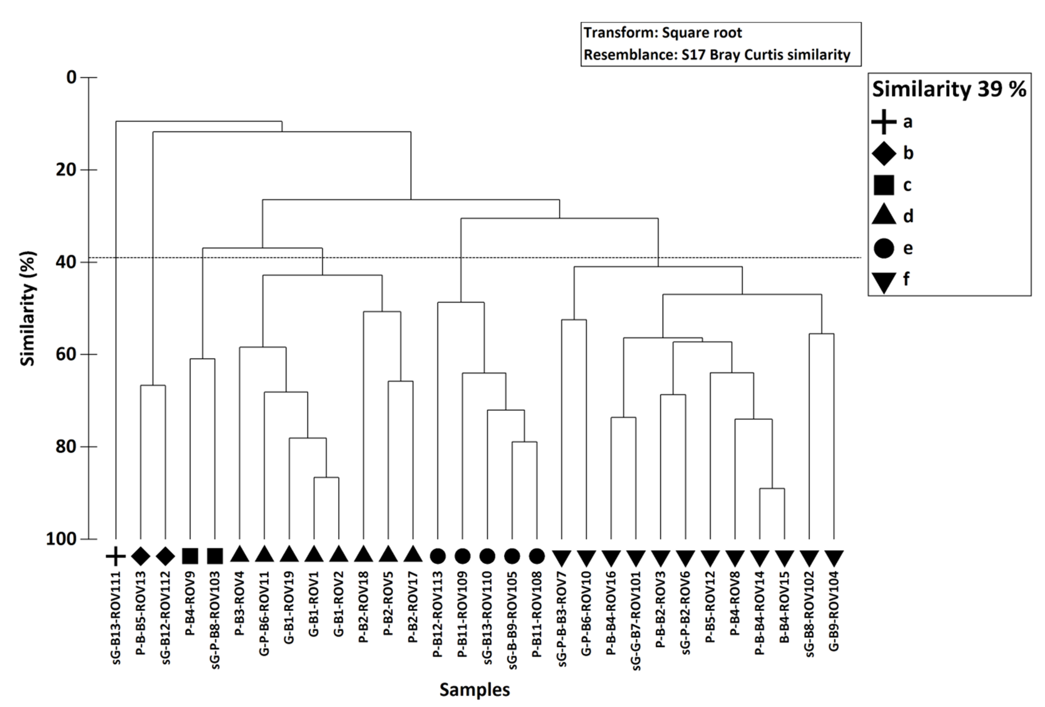
4.7. ROV Observation
5. Discussion
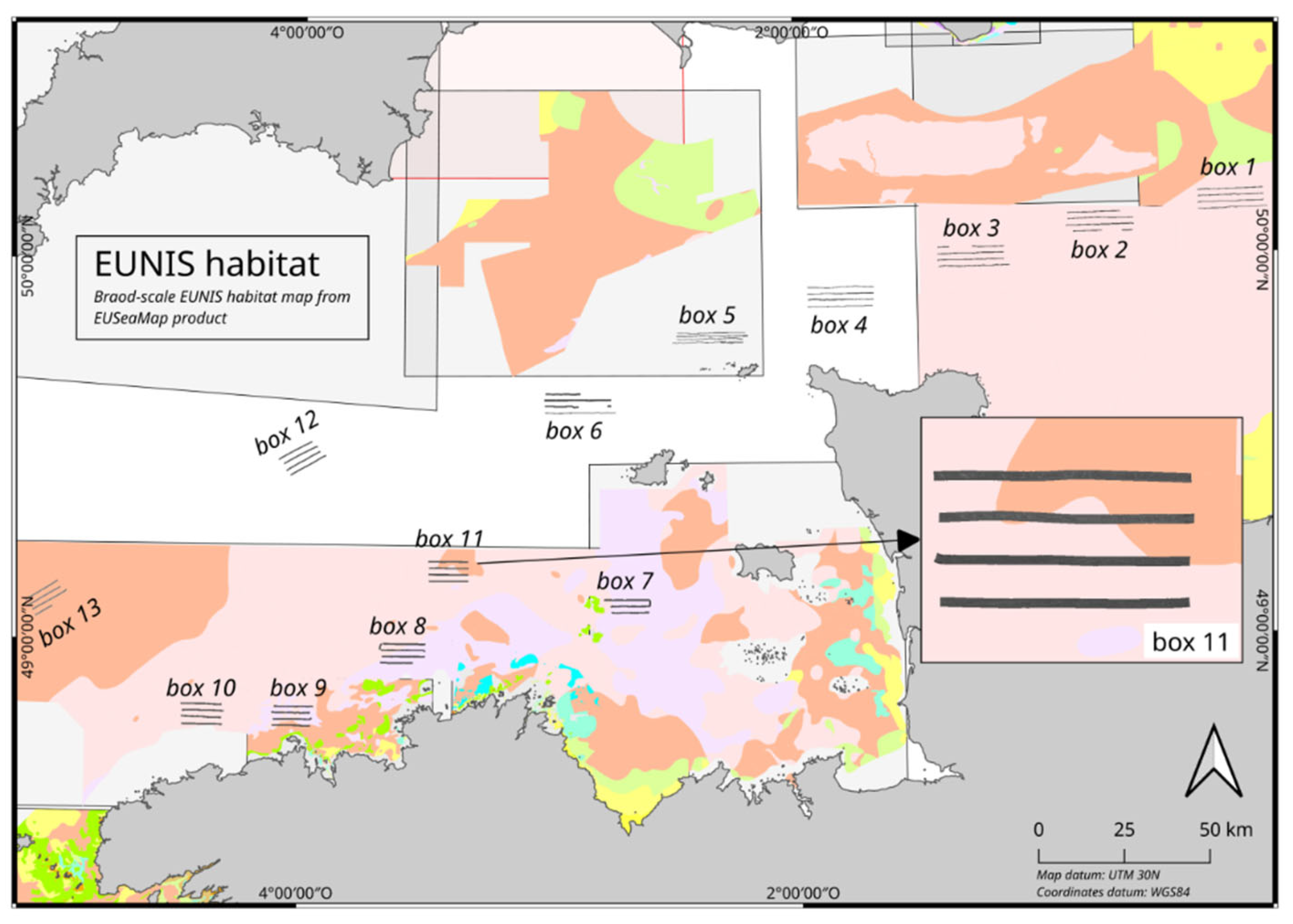
5.1. EUNIS Classification
5.2. New Quantitative Data on the Coarse Sediment of the Central Part of the English Channel
5.3. Information Gained from the Seven Benthic Habitats Sampling Methods
5.4. Perspectives on the Future of the EC Marine Management
Author Contributions
Funding
Institutional Review Board Statement
Informed Consent Statement
Data Availability Statement
Acknowledgments
Conflicts of Interest
Appendix A
| DATE | Box | Code | ST | RE | LATITUDE | LONGITUDE | Depth | SEDIMENT PHOTOS |
| 05/06/2010 | 1 | ROV1 | 2 | 1 | 50.14906667 | −0.20678333 | 49.64 | |
| 05/06/2010 | 1 | B2H1 | 2 | H1 | 50.14915 | −0.20561667 | 46.6 | gravel, coarse sand: sandy gravel |
| 05/06/2010 | 1 | B2H2 | 2 | H2 | 50.14915 | −0.20561667 | 46.6 | coarse sand, gravel: sandy gravel |
| 05/06/2010 | 1 | B2G | 2 | G | 50.14915 | −0.20561667 | 46.6 | coarse sand, gravel and pebbles: sandy gravel |
| 05/06/2010 | 1 | ROV1bis | 2 | 2 | 50.14933333 | −0.20676667 | 48.93 | |
| 05/06/2010 | 1 | B3H1 | 3 | H1 | 50.13373333 | −0.14618333 | 50.12 | coarse sand, gravel and shells: sandy gravel |
| 05/06/2010 | 1 | B3H2 | 3 | H2 | 50.13388333 | −0.14575 | 50.07 | coarse sand, gravel, pebbles and shells: sandy gravel |
| 05/06/2010 | 1 | B3G | 3 | G | 50.134 | −0.14526667 | 50.03 | gravel, coarse sand: sandy gravel |
| 05/06/2010 | 1 | B4G | 4 | G | 50.16738333 | −0.09878333 | 46.61 | coarse sand, gravel and pebbles: sandy gravel |
| 05/06/2010 | 1 | B4H1 | 4 | H1 | 50.16755 | −0.09776667 | 47.61 | coarse sand, gravel and pebbles: sandy gravel |
| 05/06/2010 | 1 | B4H2 | 4 | H2 | 50.16781667 | −0.0963 | 47.54 | coarse sand, gravel and pebbles: sandy gravel |
| 05/06/2010 | 1 | ROV2 | 5 | 1 | 50.13233333 | −0.28108333 | 46.55 | |
| 05/06/2010 | 1 | B5G | 5 | G | 50.13206667 | −0.28183333 | 43.88 | gravel, coarse sand, shells: sandy gravel |
| 05/06/2010 | 1 | B5H1 | 5 | H1 | 50.13206667 | −0.28183333 | 44.88 | coarse sand, gravel and pebbles: sandy gravel |
| 05/06/2010 | 1 | B5H2 | 5 | H2 | 50.13206667 | −0.28183333 | 43.88 | coarse sand, gravel: sandy gravel |
| 06/06/2010 | 2 | ROV3 | 6 | 1 | 50.11665 | −0.70995 | 54.14 | |
| 06/06/2010 | 2 | B6H1 | 6 | H1 | 50.11688333 | −0.71191667 | 53.14 | pebbles, gravel and coarse sand: sandy gravel |
| 06/06/2010 | 2 | B6G | 6 | G | 50.11651667 | −0.71616667 | 53.14 | pebbles, gravel and coarse sand: sandy gravel |
| 06/06/2010 | 2 | B6H2 | 6 | H2 | 50.11663333 | −0.71723333 | 52.14 | gravel, coarse sand, shells: sandy gravel |
| 06/06/2010 | 2 | B7H1 | 7 | H1 | 50.08251667 | −0.6385 | 48.14 | coarse sand, gravel, pebbles and shells: sandy gravel |
| 06/06/2010 | 2 | B7G | 7 | G | 50.08265 | −0.64048333 | 48.14 | gravel, coarse sand: sandy gravel |
| 06/06/2010 | 2 | B7H2 | 7 | H2 | 50.08313333 | −0.64466667 | 48.14 | coarse sand, gravel: sandy gravel |
| 06/06/2010 | 2 | B8G | 8 | G | 50.06643333 | −0.64038333 | 50.14 | gravel, coarse sand: sandy gravel |
| 06/06/2010 | 2 | B8H1 | 8 | H1 | 50.06623333 | −0.64315 | 50.14 | coarse sand and gravel: sandy gravel |
| 06/06/2010 | 2 | B8H2 | 8 | H2 | 50.0664 | −0.64425 | 50.14 | gravel, coarse sand: sandy gravel |
| 06/06/2010 | 2 | B9G | 9 | G | 50.06808333 | −0.7975 | 57.14 | gravel, coarse sand: sandy gravel |
| 06/06/2010 | 2 | B9H1 | 9 | H1 | 50.06765 | −0.79716667 | 58.14 | pebbles and gravel: gravelly pebble |
| 06/06/2010 | 2 | B9H2 | 9 | H2 | 50.06765 | −0.79725 | 58.14 | pebbles and gravel: gravelly pebble |
| 06/06/2010 | 2 | ROV4 | 9 | 1 | 50.0684 | −0.79653333 | 58.14 | |
| 06/06/2010 | 2 | ROV5 | 9 | 2 | 50.0684 | −0.79653333 | 58.14 | |
| 07/06/2010 | 3 | ROV6 | 10 | 1 | 49.98395 | −1.16641667 | 62.46 | |
| 07/06/2010 | 3 | B10H1 | 10 | H1 | 49.98326667 | −1.16828333 | 63.93 | coarse sand (mineral) |
| 07/06/2010 | 3 | B10H2 | 10 | H2 | 49.98326667 | −1.16828333 | 63.99 | coarse sand (mineral) |
| 07/06/2010 | 3 | B10G | 10 | G | 49.98326667 | −1.16828333 | 64.01 | coarse sand (mineral) |
| 07/06/2010 | 3 | B11H1 | 11 | H1 | 50.00111667 | −1.18013333 | 55.43 | pebbles, sand and gravel: sandy gravel and pebble |
| 07/06/2010 | 3 | B11H2 | 11 | H2 | 50.00178333 | −1.18365 | 57.5 | pebbles, sand and gravel: sandy gravel and pebble |
| 07/06/2010 | 3 | B11G | 11 | G | 49.99986667 | −1.17986667 | 55.59 | pebbles, sand and gravel: sandy gravel and pebble |
| 07/06/2010 | 3 | B12H1 | 12 | H1 | 49.99875 | −1.27925 | 66.9 | pebbles with incrusting fauna |
| 07/06/2010 | 3 | B12G | 12 | G | 49.99833333 | −1.28043333 | 67.93 | gravel and coarse sand: sandy gravel |
| 07/06/2010 | 3 | B12H2 | 12 | H2 | 49.99783333 | −1.28195 | 68.88 | gravel and coarse sand: sandy gravel |
| 07/06/2010 | 3 | B13G | 13 | G | 49.99888333 | −1.34813333 | 95.26 | gravel, coarse sand and mud: sandy gravel |
| 07/06/2010 | 3 | B14G | 14 | G | 50.00106667 | −1.37768333 | 74.23 | pebbles, sand and gravel: sandy gravel |
| 07/06/2010 | 3 | B14H1 | 14 | H1 | 50.00303333 | −1.3803333 | 67.16 | pebbles, sand and gravel: sandy gravel |
| 07/06/2010 | 3 | B14H2 | 14 | H2 | 50.0036 | −1.38125 | 68.13 | pebbles, sand and gravel: sandy gravel |
| 07/06/2010 | 3 | ROV7 | 14 | 1 | 50.00116 | −1.37737 | 74.25 | |
| 07/06/2010 | 3 | B15H1 | 15 | H1 | 49.999 | −1.38511667 | 75.76 | gravel and coarse sand: sandy gravel |
| 07/06/2010 | 3 | B15G | 15 | G | 49.99941667 | −1.3893 | 70.66 | pebbles, sand and gravel: sandy pebble |
| 07/06/2010 | 3 | B15H2 | 15 | H2 | 49.9992 | −1.38666667 | 74.62 | coarse sand and gravel: sandy gravel |
| 07/06/2010 | 3 | B16H1 | 16 | H1 | 49.99925 | −1.39091667 | 70.28 | pebbles, sand and gravel: sandy gravel |
| 07/06/2010 | 3 | B16H2 | 16 | H2 | 49.99963333 | −1.39353333 | 67.14 | pebbles, sand and gravel: sandy gravel |
| 07/06/2010 | 3 | B16G | 16 | G | 49.99925 | −1.39091667 | 70.28 | pebbles, sand and gravel: sandy gravel |
| 08/06/2010 | 4 | ROV8 | 17 | 1 | 49.91855 | −1.814 | 72.28 | |
| 08/06/2010 | 4 | B17G | 17 | G | 49.8834 | −1.86686667 | 68.49 | pebbles |
| 08/06/2010 | 4 | B18G | 18 | G | 49.8835 | −1.92143333 | 68.75 | pebbles, gravel and coarse sand: sandy gravel and pebbles |
| 08/06/2010 | 4 | B18H1 | 18 | H1 | 49.8835 | −1.92143333 | 68.75 | pebbles, gravel and coarse sand: sandy gravel and pebbles |
| 08/06/2010 | 4 | B18H2 | 18 | H2 | 49.8835 | −1.92143333 | 68.75 | pebbles, gravel and coarse sand: sandy gravel and pebbles |
| 08/06/2010 | 4 | B19H1 | 19 | H1 | 49.93256667 | −1.92101667 | 77.45 | pebbles, gravel: sandy gravel and pebbles |
| 08/06/2010 | 4 | B20H1 | 20 | H1 | 49.93568333 | −1.7767 | 73.2 | gravel, sand: sandy gravel + Ophiothrix fragilis |
| 08/06/2010 | 4 | B20H1 | 20 | H2 | 49.93568333 | −1.7767 | 73.2 | clean gravel: gravel |
| 08/06/2010 | 4 | B20G | 20 | G | 49.93568333 | −1.7767 | 73.2 | clean gravel: gravel |
| 08/06/2010 | 4 | B21H1 | 21 | H1 | 49.91535 | −1.69925 | 67.66 | clean pebbles, gravel and sand: sandy gravel and pebbles |
| 08/06/2010 | 4 | B21G | 21 | G | 49.91535 | −1.70026667 | 67.68 | clean pebbles, gravel and sand: sandy gravel and pebbles |
| 08/06/2010 | 4 | B21H2 | 21 | H2 | 49.926 | −1.7023 | 69.78 | clean pebbles, gravel and sand: sandy gravel and pebbles |
| 08/06/2010 | 4 | ROV9 | 21 | 1 | 49.926 | −1.7023 | 69.78 | |
| 11/06/2010 | 6 | B22G | 22 | G | 49.6074 | −2.74438333 | 66.62 | sand and gravel: gravelly sand |
| 11/06/2010 | 6 | B22H1 | 22 | H1 | 49.60488333 | −2.74753333 | 66.56 | sand and gravel: gravelly sand |
| 11/06/2010 | 6 | B22H2 | 22 | H2 | 49.60386667 | −2.74903333 | 66.48 | sand and gravel: gravelly sand |
| 11/06/2010 | 6 | B23H1 | 23 | H1 | 49.60408333 | −2.81343333 | 68.94 | sand and gravel: gravelly sand |
| 11/06/2010 | 6 | B23H2 | 23 | H2 | 49.60203333 | −2.81508333 | 67.88 | sand and gravel: gravelly sand |
| 11/06/2010 | 6 | B23G | 23 | G | 49.60851667 | −2.81373333 | 68.68 | sand and gravel: gravelly sand |
| 11/06/2010 | 6 | ROV10 | 23 | 1 | 49.61246667 | −2.81246667 | 69.08 | |
| 11/06/2010 | 6 | ROV10bis | 23 | 2 | 49.60955 | −2.8122 | 68.54 | |
| 11/06/2010 | 6 | B24G | 24 | G | 49.60771667 | −2.88858333 | 70.28 | sand and gravel: gravelly sand |
| 11/06/2010 | 6 | B24H1 | 24 | H1 | 49.60655 | −2.87145 | 70.21 | sand and gravel: gravelly sand |
| 11/06/2010 | 6 | B24H2 | 24 | H2 | 49.6097 | −2.89128333 | 70.2 | sand and gravel: gravelly sand |
| 11/06/2010 | 6 | B25G | 25 | G | 49.6065 | −2.89561667 | 71.19 | sand and gravel: gravelly sand |
| 11/06/2010 | 6 | B26G | 26 | G | 49.60831667 | −3.00031667 | 73.29 | sand and gravel: gravelly sand |
| 11/06/2010 | 6 | B27G | 27 | G | 49.62575 | −2.96721667 | 74.4 | sand and gravel: gravelly sand |
| 11/06/2010 | 6 | B28H1 | 28 | H1 | 49.62561667 | −2.87531667 | 71.64 | sand and gravel: gravelly sand |
| 11/06/2010 | 6 | B28H2 | 28 | H2 | 49.62648333 | −2.874 | 71.69 | sand and gravel: gravelly sand |
| 11/06/2010 | 6 | B28G | 28 | G | 49.62725 | −2.87323333 | 71.69 | sand and gravel: gravelly sand |
| 11/06/2010 | 6 | ROV11 | 28 | 1 | 49.62463333 | −2.874 | 72.32 | |
| 12/06/2010 | 5 | ROV12 | 29 | 1 | 49.79016667 | −2.3665 | 75.14 | |
| 12/06/2010 | 5 | ROV12bis | 29 | 2 | 49.79016667 | −2.3665 | 79.14 | |
| 12/06/2010 | 5 | B29G | 29 | G | 49.79433333 | −2.38095 | 78.14 | pebbles + incrusting fauna |
| 12/06/2010 | 5 | B30G | 30 | G | 49.79945 | −2.43516667 | 89.14 | pebbles + incrusting fauna |
| 12/06/2010 | 5 | B31G | 31 | G | 49.80186667 | −2.4638 | 89.14 | gravel and piece of biogenic (shells) sediment: gravel |
| 12/06/2010 | 5 | B31H1 | 31 | H1 | 49.80378333 | −2.4664 | 88.14 | gravel and piece of biogenic (shells) sediment: gravel |
| 12/06/2010 | 5 | B31H2 | 31 | H2 | 49.80378333 | −2.4664 | 88.14 | gravel and piece of biogenic (shells) sediment: gravel |
| 12/06/2010 | 5 | B32G | 32 | G | 49.8089 | −2.47075 | 93.14 | sand and gravel: sandy gravel |
| 12/06/2010 | 5 | B32H1 | 32 | H1 | 49.81075 | −2.47056667 | 96.14 | sand and gravel: sandy gravel |
| 12/06/2010 | 5 | ROV13 | 34 | 1 | 49.79965 | −2.22531667 | 61.14 | |
| 12/06/2010 | 5 | B36G | 36 | G | 49.80905 | −2.22628333 | 60.14 | clean gravel and pebbles: sandy gravel and pebbles |
| 12/06/2010 | 5 | B36H1 | 36 | H1 | 49.80718333 | −2.23335 | 67.64 | clean gravel and pebbles: sandy gravel and pebbles |
| 12/06/2010 | 5 | B36H2 | 36 | H2 | 49.80498333 | −2.23906667 | 66.14 | clean gravel and pebbles: sandy gravel and pebbles |
| 12/06/2010 | 5 | B37G | 37 | G | 49.81445 | −2.23598333 | 74.14 | coarse sand |
| 12/06/2010 | 5 | B38G | 38 | G | 49.816 | −2.23496667 | 82.14 | pebbles and sand: sandy gravel and pebbles |
| 12/06/2010 | 5 | B38H1 | 38 | H1 | 49.81566667 | −2.23761667 | 80.14 | pebbles and sand: sandy gravel and pebbles |
| 12/06/2010 | 5 | B38H2 | 38 | H2 | 49.81473333 | −2.24168333 | 80.14 | pebbles and sand: sandy gravel and pebbles |
| 12/06/2010 | 4 | B39G | 39 | G | 49.9168 | −1.92555 | 71.02 | pebbles + incrusting fauna |
| 12/06/2010 | 4 | ROV14 | 39 | 1 | 49.91705 | −1.92003333 | 71.3 | |
| 12/06/2010 | 4 | B41G | 41 | G | 49.88421667 | −1.77513333 | 74.74 | clean gravel: gravel |
| 12/06/2010 | 4 | B42G | 42 | G | 49.90035 | −1.708 | 68.13 | clean gravel and pebbles |
| 13/06/2010 | 4 | ROV15 | 42 | 1 | 49.89766667 | −1.70868333 | 68.52 | |
| 13/06/2010 | 4 | ROV16 | 42 | 1 | 49.90033333 | −1.71645 | 68.96 | |
| 13/06/2010 | 3 | B43G | 43 | G | 49.98391667 | −1.2842 | 51.00 | gravel and coarse sand: sandy gravel |
| 13/06/2010 | 3 | B44G | 44 | G | 50.03398333 | −1.27103333 | 62.86 | gravel and coarse sand: sandy gravel |
| 13/06/2010 | 3 | B45G | 45 | G | 50.01706667 | −1.34053333 | 67.11 | pebbles, sand and gravel: sandy pebble + Ophiothrix fragilis |
| 13/06/2010 | 3 | B46G | 46 | G | 49.98328333 | −1.34286667 | 63.36 | pebbles, sand and gravel: sandy pebble |
| 13/06/2010 | 3 | B47G | 47 | G | 50.01678333 | −1.15681667 | 62.58 | pebbles, sand and gravel: sandy pebble |
| 13/06/2010 | 2 | B48G | 48 | G | 50.11686667 | −0.89631667 | 45.7 | pebbles and coarse sand: sandy pebbles + Ophiothrix fragilis |
| 13/06/2010 | 2 | B49G | 49 | G | 50.1181 | −0.84986667 | 44.9 | pebbles and coarse sand: sandy pebbles + Ophiothrix fragilis |
| 13/06/2010 | 2 | B50G | 50 | G | 50.1029 | −0.75853333 | 50.3 | coarse sand, gravel and shells: gravelly sand |
| 13/06/2010 | 2 | B51G | 51 | G | 50.10091667 | −0.68713333 | 46.2 | pebbles, gravel and coarse sand: sandy pebbles + Ophiothrix fragilis |
| 13/06/2010 | 2 | B52G | 52 | G | 50.08298333 | −0.8852 | 55.2 | gravel with low coarse sand: gravel |
| 13/06/2010 | 2 | ROV17 | 52 | 1 | 50.08451667 | −0.88268333 | 58.8 | |
| 13/06/2010 | 2 | ROV18 | 51 | 1 | 50.09803333 | −0.6792 | 53.8 | |
| 14/10/2010 | 1 | ROV19 | 53 | 1 | 50.14986667 | −0.35148333 | 46.8 | |
| 14/10/2010 | 1 | B53G | 53 | G | 50.14876667 | −0.35038333 | 43.4 | coarse sand, gravel: gravelly sand |
| 14/10/2010 | 1 | B54G | 54 | G | 50.16706667 | −0.25016667 | 42.64 | gravel, coarse sand, shells: sandy gravel |
| 14/10/2010 | 1 | B55G | 55 | G | 50.11571667 | −0.25716667 | 45.03 | gravel, coarse sand: sandy gravel |
| 14/10/2010 | 1 | B56G | 56 | G | 50.11535 | −0.3119 | 41.91 | coarse sand, gravel and shells: gravelly sand |
| 19/06/2011 | 7 | ROV101 | 101 | 1 | 49.09993333 | −2.73045 | 59.14 | |
| 20/06/2011 | 7 | B101G | 101 | G | 49.08051667 | −2.66063333 | 54.14 | pebbles, sand and gravel: sandy gravel and pebbles + Ophiothrix fragilis |
| 20/06/2011 | 7 | B102G | 102 | G | 49.08053333 | −2.69463333 | 55.14 | pebbles, sand and gravel: sandy gravel and pebbles + Ophiothrix fragilis |
| 20/06/2011 | 7 | B102H1 | 102 | H1 | 49.08188333 | −2.6992 | 54.14 | pebbles, sand and gravel: sandy gravel and pebbles + Ophiothrix fragilis |
| 20/06/2011 | 7 | B102H2 | 102 | H2 | 49.08021667 | −2.69173333 | 57.14 | pebbles, sand and gravel: sandy gravel and pebbles + Ophiothrix fragilis |
| 20/06/2011 | 7 | B103G | 103 | G | 49.09696667 | −2.68266667 | 56.14 | pebbles, sand and gravel: sandy gravel and pebbles + Ophiothrix fragilis |
| 20/06/2011 | 7 | B104G | 104 | G | 49.09885 | −2.65931667 | 56.14 | pebbles, sand and gravel: sandy gravel and pebbles |
| 20/06/2011 | 7 | B105H1 | 105 | H1 | 49.09933333 | −2.61485 | 56.14 | pebbles, sand and gravel: sandy gravel and pebbles + Ophiothrix fragilis |
| 20/06/2011 | 7 | B105H2 | 105 | H2 | 49.09958333 | −2.6116 | 56.14 | gravel and coarse sand: sandy gravel and pebbles + Ophiothrix fragilis |
| 20/06/2011 | 7 | B105G | 105 | G | 49.16633333 | −2.61546667 | 56.14 | pebbles and sand: sandy gravel and pebbles + Ophiothrix fragilis |
| 20/06/2011 | 7 | B106G | 106 | G | 49.1700 | −2.61546667 | 57.14 | pebbles and sand: sandy gravel and pebbles + Ophiothrix fragilis |
| 20/06/2011 | 8 | ROV102 | 102 | 1 | 48.99886667 | −3.5102 | 76.74 | |
| 20/06/2011 | 8 | ROV103 | 103 | 2 | 48.97805 | −3.60098333 | 76.14 | |
| 21/06/2011 | 8 | B107G | 107 | G | 48.96905 | −3.5337 | 73.14 | gravel and pebbles: sandy gravel and pebbles |
| 21/06/2011 | 8 | B108G | 108 | G | 48.95188333 | −3.57421667 | 73.14 | coarse sand, gravel: sandy gravel and pebbles |
| 21/06/2011 | 8 | B108H1 | 108 | H1 | 48.9519 | −3.57325 | 72.64 | coarse sand, gravel: gravelly sand |
| 21/06/2011 | 8 | B109H1 | 109 | H1 | 48.9685 | −3.61376667 | 76.14 | coarse sand, gravel with pebbles: gravelly sand with pebbles |
| 21/06/2011 | 8 | B109G | 109 | G | 48.96731667 | −3.61525 | 76.14 | coarse sand, gravel with pebbles: gravelly sand with pebbles |
| 21/06/2011 | 8 | B109H2 | 109 | H2 | 48.96863333 | −3.6084 | 76.14 | coarse sand, gravel with pebbles: gravelly sand with pebbles |
| 21/06/2011 | 8 | B110G | 110 | G | 48.98176667 | −3.58828333 | 76.14 | coarse sand, gravel with pebbles: gravelly sand with pebbles |
| 24/06/2011 | 9 | B112G | 112 | G | 48.78071667 | −3.98513333 | 67.14 | pebbles with incrusting fauna |
| 24/06/2011 | 9 | B113G | 113 | G | 48.81758333 | −3.95718333 | 74.14 | pebbles with incrusting fauna + Ophiothrix fragilis |
| 24/06/2011 | 9 | B114H1 | 114 | H1 | 48.83406667 | −3.94606667 | 77.14 | coarse sand, gravel with pebbles: gravelly sand with pebbles |
| 24/06/2011 | 9 | B114G | 114 | G | 48.83398333 | −3.94153333 | 77.14 | coarse sand, gravel with pebbles: gravelly sand with pebbles |
| 24/06/2011 | 9 | B114H2 | 114 | H2 | 48.834 | −3.93883333 | 77.14 | coarse sand and gravel: gravelly sand |
| 24/06/2011 | 9 | ROV104 | 116 | 1 | 48.80266667 | −4.00463333 | 83.14 | |
| 24/06/2011 | 9 | ROV105 | 111 | 1 | 48.78348333 | −3.9953 | 69.14 | |
| 24/06/2011 | 9 | B117G | 117 | G | 48.83215 | −4.07756667 | 83.14 | coarse sand with pebbles: gravelly sand and pebbles |
| 25/06/2011 | 10 | B118G | 118 | G | 48.83671667 | −4.37348333 | 93.14 | coarse sand, gravel with pebbles: gravelly sand with pebbles |
| 25/06/2011 | 10 | B119H1 | 119 | H1 | 48.80138333 | −4.3521 | 89.14 | coarse sand with rare pebbles: sandy gravel and pebbles |
| 25/06/2011 | 10 | B119G | 119 | G | 48.80155 | −4.35165 | 89.14 | coarse sand with rare gravel: sandy gravel and pebbles |
| 25/06/2011 | 10 | B119H2 | 119 | H2 | 48.80155 | −4.351 | 89.14 | coarse sand, gravel with pebbles: gravelly sand with pebbles |
| 25/06/2011 | 10 | B120G | 120 | G | 48.80156667 | −4.38251667 | 89.14 | coarse sand, gravel with pebbles: gravelly sand with pebbles |
| 25/06/2011 | 10 | B120H1 | 120 | H1 | 48.80116667 | −4.38211667 | 90.14 | coarse sand, gravel with pebbles: gravelly sand with pebbles |
| 25/06/2011 | 10 | B120H2 | 120 | H2 | 48.80103333 | −4.38196667 | 90.14 | coarse sand, gravel with pebbles: gravelly sand with pebbles |
| 25/06/2011 | 10 | B121G | 121 | G | 48.8035 | −4.44663333 | 91.14 | coarse sand, gravel with pebbles: gravelly sand with pebbles |
| 25/06/2011 | 11 | B123G | 123 | G | 49.2176 | −3.47475 | 74.14 | coarse sand with pebbles: gravelly sand and pebbles |
| 26/06/2011 | 11 | B124G | 124 | G | 49.21748333 | −3.40815 | 71.14 | coarse sand with rare pebbles: gravelly sand and pebbles |
| 26/06/2011 | 11 | B125G | 125 | G | 49.21843333 | −3.38245 | 72.14 | coarse sand with rare pebbles: gravelly sand and pebbles |
| 26/06/2011 | 11 | B125H1 | 125 | H1 | 49.21878333 | −3.38706667 | 71.14 | pebbles and coarse sand: gravelly sand and pebbles |
| 26/06/2011 | 11 | B125H2 | 125 | H2 | 49.21883333 | −3.38893333 | 72.14 | pebbles and coarse sand: gravelly sand and pebbles |
| 26/06/2011 | 11 | B126H1 | 126 | H1 | 49.2001 | −3.38335 | 71.14 | coarse sand (biogenic) |
| 26/06/2011 | 11 | B126H2 | 126 | H2 | 49.2002 | −3.38675 | 71.14 | coarse sand (biogenic) |
| 26/06/2011 | 11 | B126G | 126 | G | 49.20013333 | −3.38831667 | 72.14 | coarse sand (biogenic) |
| 26/06/2011 | 11 | ROV108 | 126 | 1 | 49.20013333 | −3.37973333 | 72.14 | |
| 26/06/2011 | 11 | ROV109 | 128 | 1 | 49.18188333 | −3.41553333 | 73.14 | |
| 26/06/2011 | 11 | B128G | 128 | G | 49.18428333 | −3.4119 | 74.14 | coarse sand (biogenic) with pebbles |
| 26/06/2011 | 11 | B129H1 | 129 | H1 | 49.16468333 | −3.43968333 | 76.14 | coarse sand with pebbles |
| 26/06/2011 | 11 | B129G | 129 | G | 49.16508333 | −3.43923333 | 76.14 | coarse sand, gravel with pebbles: gravelly sand with pebbles |
| 27/06/2011 | 13 | ROV110 | 130 | 1 | 49.09433333 | −5.05886667 | 102.14 | |
| 27/06/2011 | 13 | ROV111 | 131 | 1 | 49.10693333 | −5.03501667 | 100.43 | |
| 27/06/2011 | 13 | B130H1 | 130 | H1 | 49.09991667 | −5.00065 | 100.18 | coarse sand, gravel with pebbles and shells: gravelly sand |
| 27/06/2011 | 13 | B130H1 | 130 | H2 | 49.09955 | −4.99801667 | 100.15 | coarse sand with gravel and shells: gravelly sand |
| 27/06/2011 | 13 | B130G | 130 | G | 49.09928333 | −4.99576667 | 100.11 | coarse sand with gravel and shells: gravelly sand |
| 27/06/2011 | 13 | B131H1 | 131 | H1 | 49.10596667 | −5.03701667 | 95.53 | coarse sand (biogenic) |
| 27/06/2011 | 13 | B131H2 | 131 | H2 | 49.10588333 | −5.0351 | 95.03 | coarse sand (biogenic) |
| 27/06/2011 | 13 | B131G | 131 | G | 49.10586667 | −5.03308333 | 96.03 | coarse sand (biogenic) |
| 27/06/2011 | 13 | B132G | 132 | G | 49.12751667 | −4.98456667 | 99.02 | coarse sand, gravel: gravelly sand |
| 27/06/2011 | 13 | B133H1 | 133 | H1 | 49.13601667 | −4.9648 | 96.04 | coarse sand (biogenic) |
| 27/06/2011 | 13 | B133H2 | 133 | H2 | 49.13605 | −4.96331667 | 100.04 | medium sand with pebbles |
| 27/06/2011 | 13 | B133G | 133 | G | 49.13615 | −4.9621 | 99.06 | medium sand with shells |
| 27/06/2011 | 13 | B134H1 | 134 | H1 | 49.1221 | −4.94716667 | 99.12 | coarse sand, gravel: gravelly sand |
| 27/06/2011 | 13 | B134H2 | 134 | H2 | 49.122 | −4.94568333 | 99.14 | gravel with coarse sand: sandy gravel |
| 27/06/2011 | 13 | B134G | 134 | G | 49.12195 | −4.9425 | 101.43 | coarse sand, gravel: gravelly sand |
| 27/06/2011 | 12 | ROV112 | 135 | 1 | 49.50126 | −3.95402 | 92.41 | |
| 27/06/2011 | 12 | ROV113 | 136 | 1 | 49.51450 | −3.942804 | 95.22 |
Appendix B
| Box | Station | Pebbles | Large Gravel | Gravel | Sand | Silt–Clay | Sediment Type |
| 1 | 2 | 0 | 37.21 | 11.66 | 49.24 | 1.89 | Sandy Gravel |
| 3 | 0 | 28.83 | 13.54 | 56.37 | 1.27 | Sandy Gravel | |
| 4 | 0 | 59.07 | 7.04 | 32.73 | 1.16 | Sandy Gravel | |
| 5 | 0 | 67.84 | 8.30 | 22.81 | 1.06 | Sandy Gravel | |
| 2 | 6 | 0 | 74.47 | 2.64 | 22.25 | 0.64 | Sandy Gravel |
| 7 | 0 | 63.91 | 9.16 | 26.77 | 0.16 | Sandy Gravel | |
| 8 | 0 | 59.08 | 9.92 | 30.96 | 0.04 | Sandy Gravel | |
| 9 | 0 | 46.07 | 18.49 | 35.13 | 0.31 | Sandy Gravel | |
| 3 | 10 | 0 | 0.32 | 54.77 | 44.91 | 0 | Sandy Gravel |
| 11 | 0 | 81.12 | 6.58 | 12.13 | 0.17 | Gravel | |
| 12 | 0 | 76.21 | 9.75 | 13.55 | 0.49 | Gravel | |
| 14 | 0 | 77.13 | 8.58 | 13.50 | 0.79 | Gravel | |
| 15 | 0 | 81.99 | 5.88 | 12.05 | 0.08 | Gravel | |
| 16 | 0 | 62.88 | 6.14 | 30.87 | 0.11 | Sandy Gravel | |
| 4 | 18 | 0 | 95.12 | 1.23 | 3.53 | 0.13 | Gravel |
| 19 | 0 | 94.55 | 1.19 | 4.02 | 0.24 | Gravel | |
| 20 | 0 | 78.77 | 7.74 | 13.45 | 0.04 | Gravel | |
| 21 | 0 | 50.00 | 46.52 | 3.47 | 0.01 | Gravel | |
| 5 | 31 | 0 | 91.66 | 5.27 | 2.95 | 0.12 | Gravel |
| 32 | 0 | 67.04 | 8.03 | 24.50 | 0.43 | Sandy Gravel | |
| 36 | 0 | 83.65 | 1.19 | 15.13 | 0.02 | Gravel | |
| 38 | 0 | 84.78 | 4.64 | 10.58 | 0.01 | Gravel | |
| 6 | 22 | 0 | 41.52 | 12.70 | 44.02 | 1.76 | Sandy Gravel |
| 23 | 0 | 22.97 | 9.80 | 67.07 | 0.16 | Sandy Gravel | |
| 24 | 0 | 37.40 | 13.80 | 48.21 | 0.58 | Sandy Gravel | |
| 28 | 0 | 47.17 | 13.44 | 39.14 | 0.26 | Sandy Gravel | |
| 7 | 102 | 16.64 | 22.77 | 9.80 | 50.35 | 0.44 | Sandy Gravel and Pebbles |
| 105 | 53.60 | 10.67 | 8.67 | 26.58 | 0.48 | Sandy Gravel and Pebbles | |
| 8 | 108 | 8.59 | 49.44 | 11.20 | 30.71 | 0.06 | Sandy Gravel and Pebbles |
| 109 | 8.91 | 35.63 | 17.42 | 37.93 | 0.11 | Sandy Gravel and Pebbles | |
| 9 | 114 | 40.15 | 18.62 | 9.99 | 31.21 | 0.02 | Sandy Gravel and Pebbles |
| 10 | 119 | 26.97 | 10.64 | 8.85 | 53.52 | 0.03 | Sandy Gravel and Pebbles |
| 120 | 42.94 | 7.36 | 2.94 | 46.74 | 0.02 | Sandy Gravel and Pebbles | |
| 11 | 125 | 21.54 | 6.73 | 13.74 | 57.98 | 0.02 | Sandy Gravel and Pebbles |
| 126 | 0 | 1.92 | 17.16 | 80.89 | 0.03 | Gravelly Sand | |
| 129 | 37.05 | 7.15 | 5.24 | 50.52 | 0.03 | Sandy Gravel and Pebbles | |
| 130 | 17.97 | 10.48 | 12.30 | 58.84 | 0.41 | Sandy Gravel and Pebbles | |
| 13 | 131 | 0 | 4.92 | 15.65 | 79.35 | 0.07 | Gravelly Sand |
| 133 | 8.39 | 10.96 | 11.31 | 68.77 | 0.57 | Sandy Gravel and Pebbles | |
| 134 | 28.40 | 17.55 | 8.96 | 44.65 | 0.45 | Sandy Gravel and Pebbles |
References
- Carpentier, A.; Vaz, S.; Martin, C.S.; Coppin, F.; Dauvin, J.C.; Desroy, N.; Dewarumez, J.M.; Eastwood, P.D.; Ernande, B.; Harrop, S.; et al. Eastern Channel Habitat Atlas for Marine Resource Management (CHARM). Report INTERREG IIIA; IFREMER: Brest, France, 2005; 225p. [Google Scholar]
- Carpentier, A.; Martin, C.S.; Vaz, S. (Eds.) Channel Habitat Atlas for Marine Resource Management, Final Report (CHARM Phase II); INTERREG 3 A Programme; IFREMER: Boulogne-sur-mer, France, 2009; 626p. [Google Scholar]
- Martin, C.S.; Carpentier, A.; Vaz, S.; Coppin, F.; Curet, L.; Dauvin, J.C.; Delavenne, J.; Dewarumez, J.M.; Dupuis, L.; Engelhard, G.; et al. The Channel habitat atlas for marine resource management (CHARM): An aid for planning and decision-making in an area under strong anthropogenic pressure. Aquat. Liv. Res. 2009, 22, 499–508. [Google Scholar] [CrossRef]
- Martin, C.; Meaden, G.; Vaz, S.; Dupuis, L.; Lauria, V.; Ernande, B.; Dauvin, J.C.; Spilmont, N.; Dewarumez, J.M.; Foveau, A.; et al. Channel Habitat Atlas for Marine Resources Management (CHARM)–An Aid to Management of a Resource Stressed Marine Area. In Ocean Globe; Breman, J., Ed.; ESRI Press Academic: Redlands, CA, USA, 2010; pp. 57–73. [Google Scholar]
- Delavenne, J.; Metcalfe, K.; Smith, R.J.; Vaz, S.; Martin, C.S.; Dupuis, L.; Coppin, F.; Carpentier, A. Systematic conservation planning in the eastern English Channel: Comparing the Marxan and Zonation decision-support tools. ICES J. Mar. Sci. 2012, 69, 75–83. [Google Scholar] [CrossRef]
- Foveau, A.; Vaz, S.; Desroy, N.; Kostylev, V.E. Process-driven and biological characterisation and mapping of seabed habitats sensitive to trawling. PLoS ONE 2018, 12, e0184486. [Google Scholar] [CrossRef] [PubMed]
- Holme, N.A. The bottom fauna of the English Channel. J. Mar. Biol. Assoc. UK 1961, 41, 397–461. [Google Scholar] [CrossRef]
- Holme, N.A. The bottom fauna of the English Channel. Part II. J. Mar. Biol. Assoc. UK 1966, 46, 406–493. [Google Scholar] [CrossRef]
- Cabioch, L. Contribution à la connaissance des peuplements benthiques de la Manche occidentale. Cah. Biol. Mar. 1968, 9, 493–720. [Google Scholar]
- Cabioch, L.; Gentil, F.; Glaçon, R.; Retière, C. Le macrobenthos des fonds meubles de la Manche, distribution générale et écologie. In Biology of Benthic Organisms; Keegan, B., O’Ceidigh, P., Boaden, P., Eds.; Pergamon Press: Oxford, UK, 1977; pp. 115–128. [Google Scholar]
- Coggan, R.; Diesing, M. The seabed habitats of the central English Channel: A generation on from Holme and Cabioch, how do their interpretations match-up to modern mapping techniques. Cont. Shelf Res. 2011, 31, S132–S150. [Google Scholar] [CrossRef]
- Lozach, S.; Dauvin, J.C.; Méar, Y.; Murat, A.; Dominique Davoult, D.; Migné, A. Sampling epifauna, a necessity for a better assessment of benthic ecosystem functioning: An example of the epibenthic aggregated species Ophiothrix fragilis from the Bay of Seine. Mar. Poll. Bull. 2011, 62, 2753–2760. [Google Scholar] [CrossRef]
- Lozach, S.; Dauvin, J.C. Temporal stability of a coarse sediment community from the central eastern English Channel palleovalleys. J. Sea Res. 2012, 71, 14–24. [Google Scholar] [CrossRef]
- Coggan, R.; Populus, J.; White, J.; Sheehan, K.; Fitzpatrick, F.; Piel, S. (Eds.) Review of Standards and Protocols for Seabed Habitat Mapping. MESH. 2007. Available online: http://www.searchmesh.net/ (accessed on 1 February 2022).
- Holme, N.A.; Barrett, R.L. A sledge with television and photographic cameras for quantitative investigation of the epifauna on the continental shelf. J. Mar. Biol. Assoc. UK 1977, 57, 391–403. [Google Scholar] [CrossRef]
- Cabioch, L. Résultats obtenus par l’emploi de la photographie sous-marine sur les fonds du large de Roscoff. Helgol. Meeresun. 1967, 15, 361–370. [Google Scholar] [CrossRef]
- Brown, C.J.; Cooper, K.M.; Meadows, W.J.; Limpenny, D.S.; Rees, H.L. Small-scale mapping of sea-bed assemblages in the Eastern English Channel using sidescan sonar and remote sampling techniques. Estuar. Coast. Shelf Sci. 2002, 54, 263–278. [Google Scholar] [CrossRef]
- Brown, C.J.; Hewer, A.J.; Limpenny, D.S.; Cooper, K.M.; Rees, H.L.; Meadows, W.J. Mapping seabed biotopes using sidescan sonar in responses of heterogeneous substrata: Case study east offs the Isle of Wight, English Channel. Underw. Technol. Int. J. Soc. Under. 2004, 26, 27–36. [Google Scholar] [CrossRef]
- Brown, C.J.; Hewer, A.J.; Meadows, W.J.; Limpenny, D.S.; Cooper, K.M.; Rees, H.L. Mapping seabed biotopes at Hastings Shingle Bank, eastern English Channel. Part 1. Assessment using side scan sonar. J. Mar. Biol. Assoc. UK 2004, 84, 481–488. [Google Scholar] [CrossRef]
- Brown, C.J.; Smith, S.J.; Lawton, P.; Anderson, J.T. Benthic habitat mapping: A review of progress towards improved understanding of the spatial ecology of the seafloor using acoustic techniques. Estuar. Coast. Shelf Sci. 2011, 92, 502–520. [Google Scholar] [CrossRef]
- Ehrhold, A.; Hamon, D.; Guillaumont, B. The REBENT monitoring network, a spatially integrated, acoustic approach to surveying nearshore macrobenthic habitats: Application to the Bay of Concarneau (South Brittany, France). ICES J. Mar. Sci. 2006, 63, 1604–1615. [Google Scholar] [CrossRef]
- Schumchenia, E.J.; King, J.W. Comparison of methods for integrating biological and physical data for marine habitat mapping and classification. Cont. Shelf Sci. 2010, 30, 1717–1729. [Google Scholar] [CrossRef]
- Coggan, R.; Diesing, M. Rock ridges in the Central English Channel. In Seafloor Geomorphology as Benthic Habitats; Harris, P.T., Baker, E.K., Eds.; Elsevier: Amsterdam, The Netherlands, 2012; pp. 471–480. [Google Scholar]
- Coggan, R.; Barrio Frojan, R.S.; Diesing, M.; Aldridge, J. Spatial patterns in gravels habitats and communities in the central and eastern English Channel. Estuar. Coast. Shelf Sci. 2012, 111, 118–128. [Google Scholar] [CrossRef]
- Foveau, A. Habitats et Communautés Benthiques du Bassin Oriental de la Manche: État Des Lieux au Début du XXIème Siècle. Ph.D. Thesis, University of Lille 1, Lille, France, 2009. [Google Scholar]
- Foveau, A.; Desroy, N.; Dauvin, J.C.; Dewarumez, J.M. Distribution patterns in the benthic diversity of the eastern English Channel. Mar. Ecol. Progr. Ser. 2013, 479, 115–126. [Google Scholar] [CrossRef]
- Dauvin, J.C. Are the Eastern and Western Basins of the English Channel Two Separate Ecosystems? Mar. Poll. Bull. 2012, 64, 463–471. [Google Scholar] [CrossRef]
- Dauvin, J.C. History of benthic research in the English Channel: From general patterns of communities to habitat mosaic description. J. Sea Res. 2015, 100, 32–45. [Google Scholar] [CrossRef]
- Dauvin, J.C. The English Channel: La Manche. In World Seas: An Environmental Evaluation: Volume I: Europe, The Americas and West Africa; Chapter 6; Academic Press: Cambridge, MA, USA, 2018; pp. 153–188. [Google Scholar]
- Paphitis, D.; Bastos, A.C.; Evans, G.; Collins, M. The English Channel (La Manche): Evolution, oceanography and sediment dynamics–a synthesis. In Micropaleontology, Sedimentology, Environments and Stratigraphy. A tribute to Dennis Curry (1912–2001); Whittaker, J.E., Hart, M.B., Eds.; Micropalaeontological Society: London, UK, 2010; pp. 99–132. [Google Scholar]
- Larsonneur, C.; Bouysse, P.; Auffret, J.P. The superficial sediments of the English Channel and its western approaches. Sedimentology 1982, 29, 851–864. [Google Scholar] [CrossRef]
- Dauvin, J.C. (Ed.) Les biocénoses marines et littorales françaises des côtes Atlantique, Manche et Mer du Nord, synthèse, menaces et perspectives. Laboratoire de Biologie des Invertébrés Marins et Malacologie-Service du Patrimoine Naturel: IEGB/MNHN, Paris. Collect. Patrim. Nat. 1997, 28, 1–376. [Google Scholar]
- Boyd, S.E.; Coggan, R.A.; Birchenough, S.N.R.; Limpenny, D.S.; Eastwood, P.E.; Foster-Smith, R.L.; Philpott, S.; Meadows, W.J.; James, J.W.C.; Vanstaen, K.; et al. The role of seabed mapping techniques in environmental monitoring and management. Sci. Ser. Tech. Rep. CEFAS Lowestoft 2006, 127, 170. [Google Scholar]
- Van Overmeeren, R.; Craeymeersch, J.; van Dalfsen, J.; Frouke Fey, F.; van Heteren, S.; Meesters, S. Acoustic habitat and shellfish mapping and monitoring in shallow coastal water–Sidescan sonar experiences in The Netherlands. Estuar. Coast. Shelf Sci. 2009, 85, 437–448. [Google Scholar] [CrossRef]
- Freitas, R.; Ricardo, F.; Pereira, F.; Leandro Sampaio, L.; Carvalho, S.; Gaspar, M.; Quitino, V.; Rodrigues, A.M. Benthic habitat mapping: Concerns using a combined approach (acoustic, sediment and biological data). Estuar. Coast. Shelf Sci. 2011, 92, 598–606. [Google Scholar] [CrossRef]
- Blondel, P.; Murton, B.J. Handbook of Seafloor Sonar Imagery; Wiley: Chichester, UK, 1997. [Google Scholar]
- Fish, J.P.; Carr, H.A. Sound Underwater Images: A Guide to the Generation and Interpretation of Side Scan Sonar Data; Lower Cape Publishing: Orleans, France, 1990. [Google Scholar]
- Garcia, C. Approche Fonctionnelle des Communautés Benthiques du Bassin Oriental du Bassin Oriental de la Manche et Du sud de la Mer du Nord. Ph.D. Thesis, University of Lille 1, Lille, France, 2010. [Google Scholar]
- Pezy, J.P.; Dauvin, J.C. Large extent but few quantitative data: The English Channel coarse sediments. Ecol. Ind. 2021, 121, 107010. [Google Scholar] [CrossRef]
- Clarke, K.R.; Gorley, R.N. PRIMER V6: User Manual/Tutorial; PRIMER-E: Plymouth, UK, 2006. [Google Scholar]
- Galparsoro, I.; Connor, D.W.; Borja, Á.; Aish, A.; Amorim, P.; Bajjouk, T.; Chambers, C.; Coggan, R.; Dirberg, G.; Ellwood, H.; et al. Using EUNIS habitat classification for benthic mapping in European seas: Present concerns and future needs. Mar. Poll. Bull. 2012, 64, 2630–2638. [Google Scholar] [CrossRef]
- Baffreau, A.; Chouquet, B.; Dancié, C.; Duhamel, S.; Foveau, F.; Hacquebart, P.; Navon, M.; Pezy, J.P.; Poisson, A.; Marmin, S.; et al. Mapping benthic communities: An indispensable tool for the preservation and the management of the Bay of Seine eco-socio-system. Reg. Stud. Mar. Sci. 2017, 9, 162–173. [Google Scholar] [CrossRef]
- Dauvin, J.C. Structure et organisation trophique du peuplement des sables grossiers a Amphioxus lanceolatus-Venus fasciata de la Baie de Morlaix (Manche Occidentale). Cah. Biol. Mar. 1988, 29, 163–185. [Google Scholar]
- Rolet, C.; Desroy, N. Les Biocénoses Benthiques Circalittorales de la Manche, du Sud de la Mer du Nord et de la Mer d’Iroise: Synthèse des Connaissances; Rapport Ifremer RST.LER/FBN-12-008.DN; Laboratoire Environnement Ressources Finistère-Bretagne Nord, Station de Dinard et Centre de Recherche et d’Etudes des Systèmes COtiers (CRESCO): Dinard, France, 2012. [Google Scholar]
- Newell, R.C.; Seiderer, L.J. Benthic Ecology off Lowestoft Dredging Application Area 454; Report prepared for Oakwood Environmental No SCS/454/1; MESL (Marine Ecological Survey Ltd.): Wormley, UK, 1996; 48p. [Google Scholar]
- MESL. Benthic Ecology South West of the Isle of Wight. Area 465/1 & 465/2 (West Channel); Report prepared for Coastline Surveys Limited; MESL (Marine Ecological Survey Ltd.): Gloucestershire, UK, 1999; p. 39. [Google Scholar]
- Desprez, M. Physical and biological impact of marine aggregate extraction along the French coast of the eastern English Channel: Short and long-term post-dredging restoration. ICES J. Mar. Sci. 2000, 57, 1428–1438. [Google Scholar] [CrossRef]
- Desprez, M.; Pearce, B.; Le Bot, S. The biological impact of overflowing sands around a marine aggregate extraction site: Dieppe (eastern English Channel). ICES J. Mar. Sci. 2010, 67, 270–277. [Google Scholar] [CrossRef]
- Pezy, J.P.; Raoux, A.; Legrain, M.; Boisserie, R.; Dauvin, J.C. Etat initial avant exploitation, Suivi des Sédiments, des Habitats et Communautés Benthiques du Site Granulat Marin Havrais; Publication Univ Rouen Havre: Caen, France, 2021; 66p. [Google Scholar]
- Etienne, C.; In Vivo. Projet de parc éolien en mer au large de Courseulles-sur-Mer (Calvados). In Synthèse de l’expertise “Analyse des Biocénoses Benthiques 2009; Eoliennes Offshore du Calvados, La Forêt Fouesnant; Biotope Edition: Mèze, France, 2013; p. 23. [Google Scholar]
- Raoux, A.; Pezy, J.P.; Legrain, M.; Boisserie, R.; Dauvin, J.C. Etat de Référence Avant Construction MSu3, Suivi de la Qualité de l’eau, des Sédiments, des Habitats et Communautés Benthiques; Rapport de L’état de Reference; Archimer: Caen, France, 2021; 98p. [Google Scholar]
- Newell, R.C.; Seiderer, L.J.; Robinson, J.E. Animal: Sediment relationships in coastal deposits of the eastern English Channel. J. Mar. Biol. Assoc. UK 2001, 81, 1–9. [Google Scholar] [CrossRef]
- Newell, R.C.; Seiderer, L.J.; Simpson, N.M.; Robinson, J.E. Impacts of Marine Aggregate Dredging on Benthic Macrofauna off the South Coast of the United Kingdom. J. Coast. Res. 2004, 20, 115–125. [Google Scholar] [CrossRef]
- Cooper, K.; Boyd, S.; Eggleton, J.; Limpenny, D.; Rees, H.; Vanstaen, K. Recovery of the seabed following marine aggregate dredging on the Hastings Shingle Bank off the southeast coast of England. Estuar. Coast. Shelf Sci. 2007, 75, 547–558. [Google Scholar] [CrossRef]
- Dauvin, J.C.; Ruellet, T. Macrozoobenthic biomass in the Bay of Seine (eastern English Channel). J. Sea Res. 2008, 59, 320–326. [Google Scholar] [CrossRef]
- Lozach, S.; Trentesaux, A.; Baffreau, A.; Poizot, E.; Dauvin, J.C. Typologie des Habitats Benthiques Marins en Environnement Macrotidal: Approche Pluridisciplinaire dans la Partie Centrale de la Manche. Actes du Colloque Cartographie des Habitats Marins Benthiques: De l’Acquisition à la Restitution, Brest 26–28 mars 2013, pages 8–11. Available online: http://www.carhambar.org (accessed on 1 February 2022).
- Holme, N.A.; Wilson, J.B. Faunas associated with longitudinal furrows and sand ribbons in a tide-swept area in the English Channel. J. Mar. Biol. Assoc. UK 1985, 65, 1051–1072. [Google Scholar] [CrossRef]
- Diesing, M.; Coggan, R.; Vanstaen, K. Widespread rocky reef occurrence in the central English Channel and the implications for predictive habitat mapping. Estuar. Coast. Shelf Sci. 2009, 83, 647–658. [Google Scholar] [CrossRef]
- Raoux, A.; Pezy, J.P.; Robin, I.; Bennis, A.C.; Dauvin, J.C. Multidisciplinary and multi-scale assessment of marine renewable energy structure in tidal system. J. Energ. Power Tech. 2021, 3, 012. [Google Scholar] [CrossRef]
- Pezy, J.P. Approche Écosystémique d’un Futur Parc Éolien en Manche Orientale: Exemple du Site de Dieppe–Le Tréport. Ph.D. Thesis, Caen Normandy University, Caen, France, 2017. [Google Scholar]
- Sheedan, E.V.; Stevens, T.F.; Attrill, M.J. A quantitative, non-destructive methodology for habitat characterization and benthic monitoring at offshore renewable energy developments. PLoS ONE 2010, 5, e14461. [Google Scholar]


| Morphological Structures | Box | ||||||||||||
|---|---|---|---|---|---|---|---|---|---|---|---|---|---|
| N° | 1 | 2 | 3 | 4 | 5 | 6 | 7 | 8 | 9 | 10 | 11 | 12 | 13 |
| Length (km) | 83.2 | 77.5 | 84.5 | 82.1 | 83.5 | 75.3 | 39.4 | 53.4 | 50.3 | 53.0 | 51.5 | 50.1 | 45.0 |
| Ribbons (km2) | 0 | - | 0 | 0 | - | - | - | - | - | - | - | - | 0 |
| Furrows (km2) | 0 | - | 0.6 | 2.56 | - | - | - | - | - | - | - | - | 0 |
| Small and medium dunes (km2) | 0 | - | 0 | 0 | - | - | - | - | - | - | - | - | 0 |
| Very large dunes (km2) | 0 | - | 1.6 | 1.3 | - | - | - | - | - | - | - | - | 16.4 |
| Sand veneer on rocks | 0 | - | 0 | 0 | - | - | - | - | - | - | - | - | 0 |
| Homogeneous zone (km2) | 0 | - | 0 | 0 | - | - | - | - | - | - | - | - | 0 |
| Table rocks, outcropping or sub-flush rocks (km2) | 0 | - | 2.6 | 3.26 | - | - | - | - | - | - | - | - | 0 |
| Rocky area (km2) | 0 | - | 0.5 | 4.55 | - | - | - | - | - | - | - | - | 0 |
| Dredge or trawl trace (km) | 88.5 | - | 3.0 | 1.0 | - | - | - | - | - | - | - | - | 3.14 |
| Wreck or anthropic marks | 25 | - | 64 | 33 | - | - | - | - | - | - | - | - | 0 |
| Main Sediment Type | Box | Station | 2 mm | 2 + 1 mm | ||||||
|---|---|---|---|---|---|---|---|---|---|---|
| TR | A | J’ | H’ | TR | A | J’ | H’ | |||
| Gravel | 3 | 11 | 53 | 104.0 ± 25.5 | 0.74 ± 0.14 | 2.17 ± 0.82 | 75 | 234.0 ± 25.5 | 0.85 ± 0.03 | 4.97 ± 0.44 |
| 12 | 60 | 135.0 ± 36.8 | 0.80 ± 0.02 | 2.49 ± 0.03 | 74 | 265.0 ± 36.8 | 0.84 ± 0.02 | 4.93 ± 0.11 | ||
| 14 | 54 | 184.5 ± 51.6 | 0.65 ± 0.01 | 2.10 ± 0.10 | 76 | 286.5 ± 88.4 | 0.77 ± 0.01 | 4.42 ± 0.15 | ||
| 15 | 21 | 19.0 ± 21.2 | 0.95 ± 0.01 | 1.41 ± 1.12 | 37 | 44.0 ± 36.8 | 0.94 ± 0.01 | 4.08 ± 0.82 | ||
| 4 | 18 | 64 | 132.5 ± 40.3 | 0.83 ± 0.01 | 2.70 ± 0.17 | 87 | 195.5 ± 27.6 | 0.86 ± 0.01 | 5.02 ± 0.11 | |
| 19 | 47 | 282.0 ± 0.0 | 0.66 ± 0.00 | 2.31 ± 0.00 | 81 | 423.0 ± 164.0 | 0.74 ± 0.07 | 4.46 ± 0.69 | ||
| 20 | 14 | 11.5 ± 3.5 | 0.97 ± 0.01 | 1.51 ± 0.23 | 27 | 39.5 ± 3.5 | 0.93 ± 0.01 | 4.24 ± 0.17 | ||
| 21 | 27 | 52.0 ± 12.7 | 0.74 ± 0.03 | 1.70 ± 0.06 | 38 | 93.0 ± 12.7 | 0.82 ± 0.03 | 3.98 ± 0.18 | ||
| 5 | 31 | 2 | 150.0 ± 0.0 | 0.40 ± 0.00 | 0.26 ± 0.00 | 2 | 150.0 ± 0.0 | 0.40 ± 0.00 | 0.40 ± 0.00 | |
| 36 | 29 | 37.0 ± 1.4 | 0.87 ± 0.04 | 2.01 ± 0.05 | 55 | 83.0 ± 29.7 | 0.89 ± 0.01 | 4.58 ± 0.29 | ||
| 38 | 22 | 65.5 ± 20.5 | 0.45 ± 0.63 | 1.14 ± 1.62 | 34 | 112.5 ± 36.1 | 0.72 ± 0.22 | 3.27 ± 1.27 | ||
| Gravelly Sand | 11 | 126 | 8 | 15.5 ± 2.1 | 0.66 ± 0.09 | 0.77 ± 0.38 | 12 | 24.0 ± 0.0 | 0.83 ± 0.01 | 2.49 ± 0.48 |
| 13 | 131 | 14 | 28.5 ± 30.4 | 0.81 ± 0.27 | 1.21 ± 0.01 | 26 | 53.5 ± 53.0 | 0.81 ± 0.24 | 3.18 ± 0.63 | |
| Sandy Gravel | 1 | 2 | 43 | 175.0 ± 147.1 | 0.60 ± 0.46 | 1.74 ± 1.41 | 69 | 230.0 ± 144.2 | 0.66 ± 0.34 | 3.69 ± 2.08 |
| 3 | 52 | 103.0 ± 17.0 | 0.89 ± 0.01 | 2.73 ± 0.02 | 68 | 170.0 ± 22.6 | 0.85 ± 0.01 | 4.80 ± 0.19 | ||
| 4 | 63 | 123.5 ± 81.3 | 0.83 ± 0.17 | 2.63 ± 0.33 | 83 | 198.5 ± 94.0 | 0.86 ± 0.10 | 5.17 ± 0.52 | ||
| 5 | 73 | 392.5 ± 200.1 | 0.66 ± 0.17 | 2.39 ± 0.51 | 81 | 445.0 ± 250.3 | 0.69 ± 0.13 | 4.06 ± 0.58 | ||
| 2 | 6 | 39 | 161.0 ± 161.2 | 0.56 ± 0.14 | 1.47 ± 0.06 | 46 | 173.0 ± 161.2 | 0.61 ± 0.18 | 2.99 ± 0.70 | |
| 7 | 44 | 147.5 ± 74.2 | 0.73 ± 0.03 | 2.21 ± 0.16 | 58 | 239.5 ± 74.2 | 0.79 ± 0.03 | 4.41 ± 0.03 | ||
| 8 | 27 | 119.0 ± 45.3 | 0.36 ± 0.10 | 0.84 ± 0.51 | 45 | 148.5 ± 54.4 | 0.53 ± 0.06 | 2.56 ± 0.61 | ||
| 9 | 47 | 80.5 ± 3.6 | 0.85 ± 0.01 | 2.43 ± 0.02 | 79 | 262.5 ± 17.7 | 0.81 ± 0.05 | 4.66 ± 0.31 | ||
| 3 | 10 | 7 | 39.0 ± 5.7 | 0.76 ± 0.01 | 1.05 ± 0.15 | 10 | 56.0 ± 7.1 | 0.79 ± 0.01 | 2.33 ± 0.45 | |
| 16 | 46 | 68.5 ± 14.8 | 0.90 ± 0.01 | 2.58 ± 0.10 | 63 | 140.0 ± 46.7 | 0.88 ± 0.06 | 4.83 ± 0.13 | ||
| 6 | 22 | 66 | 145.0 ± 76.4 | 0.68 ±0.01 | 2.18 ± 0.33 | 76 | 156.5 ± 74.2 | 0.71 ± 0.01 | 3.95 ± 0.23 | |
| 23 | 14 | 11.0 ± 1.4 | 0.95 ±0.01 | 1.39 ± 0.09 | 26 | 22.5 ± 0.7 | 0.96 ± 0.01 | 3.94 ± 0.17 | ||
| 24 | 43 | 44.0 ± 35.3 | 0.93 ± 0.02 | 2.26 ± 0.66 | 58 | 89.0 ± 50.9 | 0.89 ± 0.04 | 4.56 ± 0.39 | ||
| 28 | 56 | 94.5 ± 47.4 | 0.90 ± 0.05 | 2.76 ± 0.15 | 88 | 278.5 ± 88.4 | 0.82 ± 0.02 | 4.84 ± 0.01 | ||
| 5 | 32 | 7 | 67.0 ± 0.0 | 0.64 ± 0.00 | 1.12 ± 0.00 | 7 | 67.0 ± 0.0 | 0.64 ± 0.00 | 1.80 ± 0.00 | |
| Sandy Gravel and Pebbles | 7 | 102 | 26 | 61.5 ± 3.5 | 0.68 ± 0.04 | 1.62 ± 0.10 | 35 | 79.0 ± 14.1 | 0.76 ± 0.01 | 3.49 ± 0.04 |
| 105 | 19 | 70.5 ± 9.2 | 0.52 ± 0.07 | 1.10 ± 0.22 | 33 | 105.5 ± 19.1 | 0.68 ± 0.15 | 3.20 ± 1.04 | ||
| 8 | 108 | 9 | 16.0 ± 0.0 | 0.90 ± 0.00 | 1.46 ± 0.00 | 13 | 20.0 ± 0.0 | 0.92 ± 0.00 | 3.40 ± 0.00 | |
| 109 | 25 | 33.5 ± 34.6 | 0.89 ± 0.07 | 1.68 ± 0.64 | 35 | 52.0 ± 52.3 | 0.91 ± 0.07 | 3.76 ± 0.62 | ||
| 9 | 114 | 59 | 72.5 ± 21.9 | 0.92 ± 0.05 | 2.68 ± 0.17 | 76 | 154.5 ± 21.9 | 0.88 ± 0.03 | 5.12 ± 0.10 | |
| 10 | 119 | 35 | 45.5 ± 17.7 | 0.86 ± 0.06 | 2.08 ± 0.09 | 47 | 74.0 ± 53.7 | 0.90 ± 0.01 | 4.27 ± 0.65 | |
| 120 | 41 | 58.5 ± 82.7 | 0.44 ± 0.62 | 1.42 ± 2.01 | 68 | 99.5 ± 88.4 | 0.91 ± 0.04 | 4.65 ± 0.73 | ||
| 11 | 125 | 35 | 73.0 ± 14.1 | 0.71 ± 0.14 | 1.79 ± 0.41 | 42 | 92.0 ± 8.5 | 0.75 ± 0.13 | 3.48 ± 0.83 | |
| 129 | 32 | 41.0 ± 18.4 | 0.78 ± 0.22 | 1.77 ± 0.47 | 37 | 72.0 ± 18.4 | 0.84 ± 0.09 | 3.99 ± 0.39 | ||
| 130 | 57 | 156.0 ± 219.2 | 0.39 ± 0.55 | 1.44 ± 2.03 | 68 | 192.0 ± 236.2 | 0.84 ± 0.11 | 4.06 ± 0.78 | ||
| 13 | 133 | 29 | 43.5 ± 44.6 | 0.84 ± 0.10 | 1.74 ± 1.19 | 40 | 69.5 ± 44.5 | 0.82 ± 0.12 | 3.64 ± 1.53 | |
| 134 | 45 | 73.0 ± 2.8 | 0.89 ± 0.03 | 2.58 ± 0.06 | 68 | 123.0 ± 29.7 | 0.90 ± 0.01 | 5.01 ± 0.25 | ||
| Group a (1) | Cc (%) | Group c (2) | Cc (%) | Group e (5) | Cc (%) | Group f (4) | Cc (%) | Group g (3) | Cc (%) |
|---|---|---|---|---|---|---|---|---|---|
| Pododesmus squama | 61.44 | Echinocyamus pusillus | 64.91 | Ophiothrix fragilis | 26.90 | Echinocyamus pusillus | 17.68 | Notomastus latericeus | 8.84 |
| Balanus crenatus | 100 | Schistomeringos neglecta | 82.46 | Aonides paucibranchiata | 40.31 | Glycera lapidum | 26.16 | Balanus crenatus | 16.59 |
| Spatangus purpureus | 100 | Laonice bahusiensis | 52.70 | Jasmineira elegans | 31.76 | Lumbrineris gracilis | 21.71 | ||
| Notomastus latericeus | 60.64 | Ampelisca spinipes | 36.34 | Nemertea | 25.84 | ||||
| Lumbrineris gracilis | 67.94 | Eunice vittata | 40.76 | Glycera lapidum | 29.85 | ||||
| Aonides oxycephala | 73.19 | Laonice bahusiensis | 45.02 | Syllis spp. | 33.27 | ||||
| Eualus occultus | 78.16 | Polycirrus medusa | 49.07 | Laonice bahusiensis | 36.37 | ||||
| Pisidia longicornis | 80.72 | Cheirocratus intermedius | 53.07 | Aonides paucibranchiata | 39.20 | ||||
| Glycymeris glycymeris | 83.22 | Timoclea ovata | 56.99 | Glycymeris glycymeris | 41.95 | ||||
| Timoclea ovata | 85.73 | Pagurus cuanensis | 60.56 | Pisidia longicornis | 44.63 |
| Group a (1) | Cc (%) | Group b (3) | Cc (%) | Group c (4) | Cc (%) | Group e (2) | Cc (%) |
|---|---|---|---|---|---|---|---|
| Pododesmus squama | 61.44 | Notomastus latericeus | 6.62 | Echinocyamus pusillus | 12.48 | Polygordius | 35.19 |
| Balanus crenatus | 100.00 | Glycera lapidum | 11.78 | Glycera lapidum | 21.28 | Pisione remota | 55.06 |
| Aonides paucibranchiata | 16.56 | Ampelisca spinipes | 26.00 | Syllis spp. | 74.93 | ||
| Eulalia mustela | 21.22 | Eulalia mustela | 30.38 | Glycera lapidum | 87.46 | ||
| Syllis spp. | 25.75 | Cheirocratus | 34.43 | Timoclea ovata | 100 | ||
| Lumbrineris gracilis | 29.69 | Jasmineira elegans | 38.27 | - | - | ||
| Laonice bahusiensis | 33.54 | Syllis spp. | 41.95 | - | - | ||
| Timoclea ovata | 36.87 | Laonice bahusiensis | 44.93 | - | - | ||
| Nemertea | 40.08 | Timoclea ovata | 47.59 | - | - | ||
| Balanus crenatus | 43.09 | Eurydice pulchra | 50.24 | - | - |
| Group a (1) | Cc (%) | Group b (2) | Cc (%) | Group c (3) | Cc (%) | Group d (4) | Cc (%) | Group e (5) | Cc (%) |
|---|---|---|---|---|---|---|---|---|---|
| Balanus crenatus | 50.0 | Glycera lapidum | 21.6 | Glycera lapidum | 2.8 | Echinocyamus pusillus | 4.5 | Eulalia mustela | 7.8 |
| Pododesmus squama | 100.0 | Polygordius sp. | 43.1 | Notomastus latericeus | 5.7 | Eulalia mustela | 9.0 | Glycera lapidum | 15.7 |
| - | - | Timoclea ovata | 64.7 | Laonice bahusiensis | 8.3 | Glycera lapidum | 13.5 | Nemertea | 23.6 |
| - | - | Pisione remota | 72.3 | Nemertea | 10.8 | Cheirocratus | 17.1 | Notomastus latericeus | 31.4 |
| - | - | Syllis spp. | 79.9 | Syllis spp. | 13.3 | Caulleriella alata | 20.6 | Aonides paucibranchiata | 37.1 |
| - | - | Echinocyamus pusillus | 86.6 | Eulalia mustela | 15.7 | Ampelisca spinipes | 24.1 | Syllis spp. | 42.8 |
| - | - | Malmgreniella arenicolae | 93.3 | Lumbrineris gracilis | 18.2 | Eunice vittata | 27.5 | Opisthodonta | 48.4 |
| - | - | - | Polycirrus medusa | 20.6 | Laonice bahusiensis | 30.8 | Polygordius sp. | 52.3 | |
| - | - | - | Aonides paucibranchiata | 22.9 | Nemertea | 34.1 | Glycymeris glycymeris | 56.0 | |
| - | - | - | Websterinereis glauca | 25.1 | Syllis spp. | 37.5 | Ophiothrix fragilis | 59.7 |
| Group b (1) Cc (%) | Group c (2) | Cc (%) | Group d (3) | Cc (%) | Group e (4) | Cc (%) | Group f (5) | Cc (%) | |
|---|---|---|---|---|---|---|---|---|---|
| Alcyonium digitatum | 100 | Ophiothrix fragilis | 33.66 | Aequipecten opercularis | 35.17 | Abietinaria abietina | 43.74 | Flustrea | 34.12 |
| - | - | Alcyonium digitatum | 61.14 | Hydrozoa | 55.69 | Sponges | 79.33 | Sponges | 50.47 |
| - | - | Hydrozoa | 80.57 | Pagurus spp. | 74.43 | Alcyonium digitatum | 89.79 | Hydrozoa | 63.66 |
| - | - | Urticina felina | 100 | Asterias rubens | 84.48 | Nemertesia | 97.67 | Nemertesia | 74.97 |
| - | - | - | - | Urticina felina | 90.15 | - | - | Balanus crenatus | 82.85 |
| - | - | - | - | - | - | - | - | Spirobranchus spp. | 89.61 |
| - | - | - | - | - | - | - | - | Alcyonium digitatum | 94.90 |
| Box | Station | Photos | Sediment Type | G 2 mm | G 2 + 1 mm | G 2 + 1 mm + Epifauna | ROV | EUNIS |
|---|---|---|---|---|---|---|---|---|
| 1 | 2 | Sandy Gravel | Sandy Gravel | 3 | 3 | 3 | 3 | MD3211 (A5.151) |
| 3 | Sandy Gravel | Sandy Gravel | 3 | 3 | 3 | 3 | MD3211 (A5.151) | |
| 4 | Sandy Gravel | Sandy Gravel | 3 | 3 | 3 | 3 | MD3211 (A5.151) | |
| 5 | Sandy Gravel | Sandy Gravel | 3 | 3 | 3 | 3 | MD3211 (A5.151) | |
| 2 | 6 | Sandy Gravel | Sandy Gravel | 3 | 3 | 3 | 5 | MD3211 (A5.151) |
| 7 | Sandy Gravel | Sandy Gravel | 3 | 3 | 3 | 3 | MD3211 (A5.151) | |
| 8 | Sandy Gravel | Sandy Gravel | 3 | 3 | 3 | 3 | MD3211 (A5.151) | |
| 9 | Sandy Gravel | Sandy Gravel | 3 | 3 | 3 | 3 | MD3211 (A5.151) | |
| 3 | 10 | Coarse sand | Sandy Gravel | 2 | 2 | 2 | 5 | MC3215 (A5.145) |
| 11 | Sandy Gravel and Pebbles | Gravel | 3 | 3 | 3 | 5 | MD3211 (A5.151) | |
| 12 | Sandy Gravel | Gravel | 3 | 3 | 3 | - | MD3211 (A5.151) | |
| 14 | Sandy Gravel | Gravel | 3 | 3 | 3 | 5 | MD3211 (A5.151) | |
| 15 | Sandy Gravel | Gravel | 3 | 3 | 5 | - | MD3211 (A5.151) | |
| 16 | Sandy Gravel | Sandy Gravel | 3 | 3 | 3 | 5 | MD3211 (A5.151) | |
| 4 | 18 | Sandy Gravel and Pebbles | Gravel | 3 | 3 | 3 | 5 | MD3211 (A5.151) |
| 19 | Sandy Gravel and Pebbles | Gravel | 3 | 3 | 3 | 5 | MD3211 (A5.151) | |
| 20 | Gravel | Gravel | 5 | 3 | 5 | 5 | MC4215 (A5. 445) | |
| 21 | Sandy Gravel and Pebbles | Gravel | 5 | 3 | 3 | 2 | MC4215 (A5. 445) | |
| 5 | 31 | Gravel | Gravel | 1 | 1 | 1 | - | MC4 (A5. 44) |
| 32 | Sandy Gravel | Sandy Gravel | 1 | 1 | 1 | 1 | MC4 (A5. 44) | |
| 36 | Sandy Gravel and Pebbles | Gravel | 3 | 3 | 3 | - | MD3211 (A5.151) | |
| 38 | Sandy Gravel and Pebbles | Gravel | 3 | 3 | 5 | - | MD3211 (A5.151) | |
| 6 | 22 | Gravelly Sand | Sandy Gravel | 3 | 3 | 3 | - | MD3211 (A5.151) |
| 23 | Gravelly Sand | Sandy Gravel | 6 | 6 | 5 | 5 | MD3211 (A5.151) | |
| 24 | Gravelly Sand | Sandy Gravel | 3 | 3 | 4 | 5 | MD3211 (A5.151) | |
| 28 | Gravelly Sand | Sandy Gravel | 4 | 3 | 3 | 3 | MD3211 (A5.151) | |
| 7 | 102 | Sandy Gravel and Pebbles | Sandy Gravel and Pebbles | 5 | 3 | 5 | - | MC4215 (A5. 445) |
| 105 | Sandy Gravel and Pebbles | Sandy Gravel and Pebbles | 5 | 3 | 5 | 2 | MC4215 (A5. 445) | |
| 8 | 108 | Sandy Gravel and Pebbles | Sandy Gravel and Pebbles | 4 | 4 | 2 | - | MC3212 (A5.142) |
| 109 | Gravelly Sand and Pebbles | Sandy Gravel and Pebbles | 4 | 4 | 5 | - | MC3212 (A5.142) | |
| 9 | 114 | Gravelly Sand and Pebbles | Sandy Gravel and Pebbles | 4 | 4 | 4 | 5 | MC3212 (A5.142) |
| 10 | 119 | Sandy Gravel and Pebbles | Sandy Gravel and Pebbles | 4 | 4 | 4 | 4 | MC3212 (A5.142) |
| 120 | Gravelly Sand and Pebbles | Sandy Gravel and Pebbles | 4 | 4 | 4 | - | MC3212 (A5.142) | |
| 11 | 125 | Gravelly Sand and Pebbles | Sandy Gravel and Pebbles | 4 | 4 | 4 | - | MC3212 (A5.142) |
| 126 | Coarse Sand | Gravelly Sand | 2 | 2 | 2 | 4 | MC3215 (A5.145) | |
| 129 | Coarse Sand and Pebbles | Sandy Gravel and Pebbles | 4 | 4 | 4 | 4 | MC3212 (A5.142) | |
| 130 | Gravelly Sand | Sandy Gravel and Pebbles | 4 | 4 | 4 | 4 | MC3212 (A5.142) | |
| 13 | 131 | Coarse Sand | Gravelly Sand | 2 | 4 | 4 | 6 | MC3215 (A5.145) |
| 133 | Gravelly Sand | Sandy Gravel and Pebbles | 4 | 4 | 4 | 1 | MC3212 (A5.142) | |
| 134 | Gravelly Sand | Sandy Gravel and Pebbles | 4 | 4 | 4 | 4 | MC3212 (A5.142) |
| Site | Month | Year | Ss | D | S | TR | A (m²) | Reference | ||
|---|---|---|---|---|---|---|---|---|---|---|
| wEC | UK | West EC | - | - | - | - | sG and gS | - | 390 | MESL, 1999 [46] |
| France | Morlaix | Each month | 1977–1980 | 32.5 | 17 | Cs | 181 | 192 | Dauvin, 1988 [43] | |
| eEC | France | Dieppe | - | 1996–1997 | 0.9 | 15 | sG | 50 | 1.940 | Desprez, 2000 [47] |
| - | 1996–2001 | 0.8 | 15 | sG | 50 | 2.394 | Desprez et al., 2010 [48] | |||
| Dieppe-Le Tréport | September/October | 2014–2016 | 14 | 12–25 | sG | 277 | 2.989 | Pezy and Dauvin, 2021 [39] | ||
| February/March | 24 | gS | 224 | 1.605 | ||||||
| Bay of Seine | June–August | 2007 | 19 | 38–50 | sG | 198 | 1.309 | Lozach and Dauvin, 2012 [13] | ||
| PER Granulats du Havre | February | 2012 | 2.5 | 16–22 | sG | 117 | 777 | Pezy et al., 2021 [49] | ||
| February | 2021 | 6 | sG and gS | 157 | 1.219 | Pezy et al., 2021 [49] | ||||
| Courseulles-sur-Mer | June | 2009 | 8.1 | 22–28 | sG | 147 | 377 | In Vivo, 2013 [50] | ||
| March | 2020 | 4.5 | 22–30 | sG | 182 | 3.303 | Raoux et al., 2021 [51] | |||
| March | 2021 | 5.4 | 22–30 | sG | 159 | 2.008 | ||||
| UK | St Catherine | - | - | - | - | sG and gS | - | 4.590 | MESL, 1996 [45] | |
| West Bassurelle | - | - | - | - | sG and gS | - | 932 | MESL, 1999 [46] | ||
| Folkestone | - | - | - | - | Cs | - | 3.051 | Newell et al., 2001 [52] | ||
| Isle of Wight | March and September | 1999 | 26.2 | >10 | Cs | 316 | 998 | Newell et al., 2004 [53] | ||
| Hastings | - | - | - | - | sG | - | 2.000 | Cooper et al., 2007 [54] | ||
| Offshore central and western part of the EC | June | 2010–2011 | 1.5 | 64–95 | Cs | 33 | 223 | This study | ||
| 1 | 88–96 | G | 7 | 434 | ||||||
| 10.5 | 45–80 | sG | 233 | 800 | ||||||
| 5 | 73–101 | sG and P | 164 | 380 | ||||||
| 2 | 54–67 | sG and P + O | 80 | 316 | ||||||
Publisher’s Note: MDPI stays neutral with regard to jurisdictional claims in published maps and institutional affiliations. |
© 2022 by the authors. Licensee MDPI, Basel, Switzerland. This article is an open access article distributed under the terms and conditions of the Creative Commons Attribution (CC BY) license (https://creativecommons.org/licenses/by/4.0/).
Share and Cite
Dauvin, J.-C.; Pezy, J.-P.; Poizot, E.; Lozach, S.; Trentesaux, A. A Multidisciplinary Approach for A Better Knowledge of the Benthic Habitat and Community Distribution in the Central and Western English Channel. J. Mar. Sci. Eng. 2022, 10, 1112. https://doi.org/10.3390/jmse10081112
Dauvin J-C, Pezy J-P, Poizot E, Lozach S, Trentesaux A. A Multidisciplinary Approach for A Better Knowledge of the Benthic Habitat and Community Distribution in the Central and Western English Channel. Journal of Marine Science and Engineering. 2022; 10(8):1112. https://doi.org/10.3390/jmse10081112
Chicago/Turabian StyleDauvin, Jean-Claude, Jean-Philippe Pezy, Emmanuel Poizot, Sophie Lozach, and Alain Trentesaux. 2022. "A Multidisciplinary Approach for A Better Knowledge of the Benthic Habitat and Community Distribution in the Central and Western English Channel" Journal of Marine Science and Engineering 10, no. 8: 1112. https://doi.org/10.3390/jmse10081112