Remote-Sensing Measurements of Wave Breaking at Two Pacific Northwest Jettied Inlets

Abstract

Breaking waves constitute one of the main environmental stressors on coastal structures as well as a leading hazard to navigation in nearshore regions. In this paper, we use camera-based methods to measure wave breaking over two jetty systems in the Pacific Northwest; the North jetty of the Columbia River, Washington state, and the two jetties of Coos Bay, Oregon, as well as over three nearby nearshore dredge disposal areas. Data were collected using the “brightest” images and Argus camera technology over a span of 847 days for the Columbia River and 202 days for Coos Bay. Wave breaking over the Columbia north jetty reached 100% for wave heights greater than 3 m and for tides above mid-tide level and was concentrated on the seaward half of the jetty. For Coos Bay, the south jetty saw substantially more breaking than the north one with the worst overtopping occurring mid-jetty and seeming to be associated with sediment transport through the jetty and into the inlet, as well as possibly the navigation channel. Wave breaking at the Coos Bay inlet mouth was enhanced during ebb flow conditions. Argus imagery analysis showed no evidence of enhanced breaking over any of the three dredge material placement sites.

1. Introduction

Coastal ocean inlets are important conduits for navigation and venues for marine recreation. In many cases, especially for commercially-important waterways supporting deep draft navigation, coastal inlets must be stabilized and secured by jetties to redirect currents, control sediment movement, and establish reliable and safe navigation channels [1]. Jetties can be subjected to tremendous loading, principally due to wave breaking, and must be built of large armor rock and/or specialized armor units to withstand these forces. The uncertainty in understanding wave breaking characteristics along coastal structures can lead to uninformed design assumptions, resulting in the implementation of non-resilient features that experience higher rates of degradation than expected. The consequence of an unraveling coastal jetty can be costly and reduce navigation safety at the affected inlet. A damaged jetty can release sediment into the inlet navigation channel and allow unfavorable wave action and currents to enter the inlet. Maintaining an under-designed and degrading jetty is an expensive proposition [2].

In turn, navigation channels at coastal inlets may require regular dredging to maintain depth. The dredged sediment (sand) is viewed as a resource for the littoral zone and is often strategically placed at permitted or designated sites within nearshore coastal waters near the inlet in order to sustain the sediment budget along the coastal zone adjoining the inlet. Regardless of the beneficial intent of re-introducing dredged sediment to the nearshore littoral zone, if the placement of dredged sediment significantly reduces water depth (via depositional mounding) at a given nearshore site, the result could alter wave propagation over the site and cause waves to break. While inducing breaking wave conditions within nearshore dredged material placement sites may increase the shoreward transport of sediment (a beneficial effect), wave breaking could impose a hazard for mariners and navigation (a far more detrimental effect). A primary tenant governing use of nearshore placement sites in the Pacific Northwest is to not alter wave characteristics in ways that could pose a hazard to navigation, due to enhanced wave breaking [3].

Both of these potential wave breaking issues are of particular interest in the Pacific Northwest (PNW) region of the United States (Washington, Oregon, and Northern California) where wave energies are the highest of any US coast [1]. To address these wave breaking concerns, Argus stations were installed at each of the two large PNW inlets (Figure 1) to observe and measure wave breaking on inlet jetties and over nearshore dredged material placement sites. The purpose of this paper is to describe the inlets, the sampling strategies, and the primary results, with the primary goals being to detect anomalous breaking over dredge disposal sites and to characterize wave breaking over three rubble mound jetties.

The next section describes the sites and the sampling approaches used. This is followed by the main results, first regarding disposal sites and second, regarding jetty breaking. These sections are followed by a discussion and conclusions.

Figure 1. Map views of the two field sites. (a) Shows the entire Pacific Northwest region and the locations of both North Head and Coos Bay. (b) Zooms in to the North Head region showing the imaged field of view to the south (white lines) spanning Benson Beach which lies between the Head and the north jetty of the Columbia River. (c) Shows a magnified view of Coos Bay including the two jetties, the navigation channels (in red), and the fields of view of the six Argus cameras (paired colored lines).

Figure 1. Map views of the two field sites. (a) Shows the entire Pacific Northwest region and the locations of both North Head and Coos Bay. (b) Zooms in to the North Head region showing the imaged field of view to the south (white lines) spanning Benson Beach which lies between the Head and the north jetty of the Columbia River. (c) Shows a magnified view of Coos Bay including the two jetties, the navigation channels (in red), and the fields of view of the six Argus cameras (paired colored lines).

2. Site Descriptions and Methods

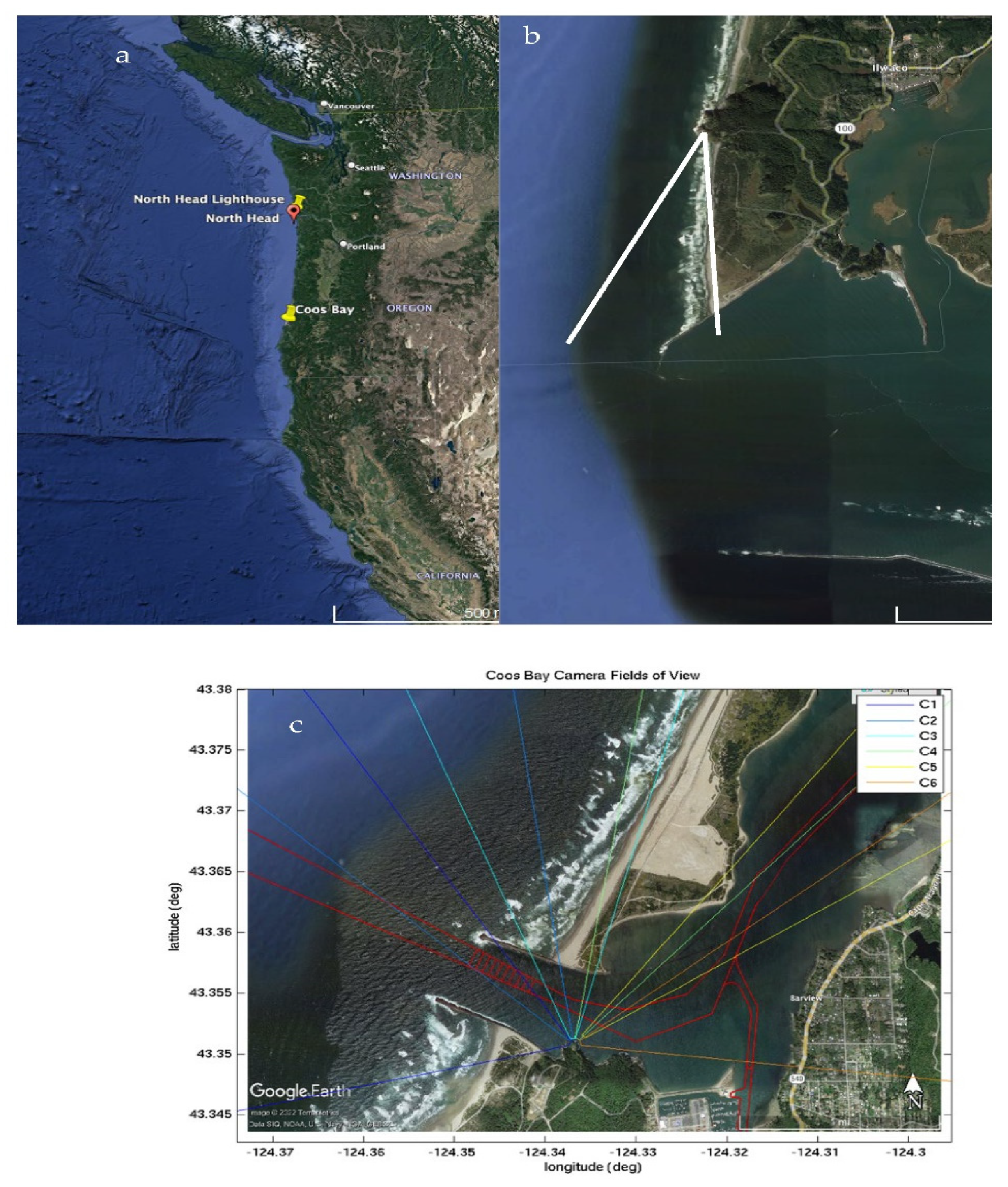
2.1. Site Descriptions

The two camera installations are at the North Head lighthouse, Washington State, and the coast guard watch station at Coos Bay, Oregon, both in the region of large wave energy in the Pacific Northwest (Figure 1a). The North Head Argus station is located 3.3 km north of the north jetty of the Columbia River and overlooks Benson Beach, a low sloping, dissipative, west-facing beach with open wave exposure to the Pacific Ocean (Figure 1b). The Coos Bay Argus station is 325 km to the south and includes an estuary opening to the WNW that connects to the long estuary of Coos Bay that winds north and then turns south (Figure 1c).

Wave heights in the PNW vary seasonally from average heights of 1.5 to 2.0 m in summer months and 2.5 to 4.0 m in winter months (e.g., [4]). However, storms can be extreme, with significant wave heights commonly ranging from 5 to 10 m and peaking at 14 to 15 m, and these magnitudes have been shown to be increasing [5]. Due to the long fetch of the Pacific Ocean, the largest storms often have periods of 15 to 17 s, but wave periods can at times exceed 20 s periods during winter months [4].

For North Head, wave height data for this study were extracted from CSIRO WaveWatch III model data for node 46.0° N, 124.8° W while tide data came from NOAA gauge 9440581 for Cape Disappointment, Washington. For the Coos Bay component of this study, tide data were obtained from NOAA tide gauge 9432780, located just inside the Charleston, Oregon, harbor mouth. Wave data were obtained from CAWCR Global Wave Hindcast model for model node point 44.0° N, 125.2° W.

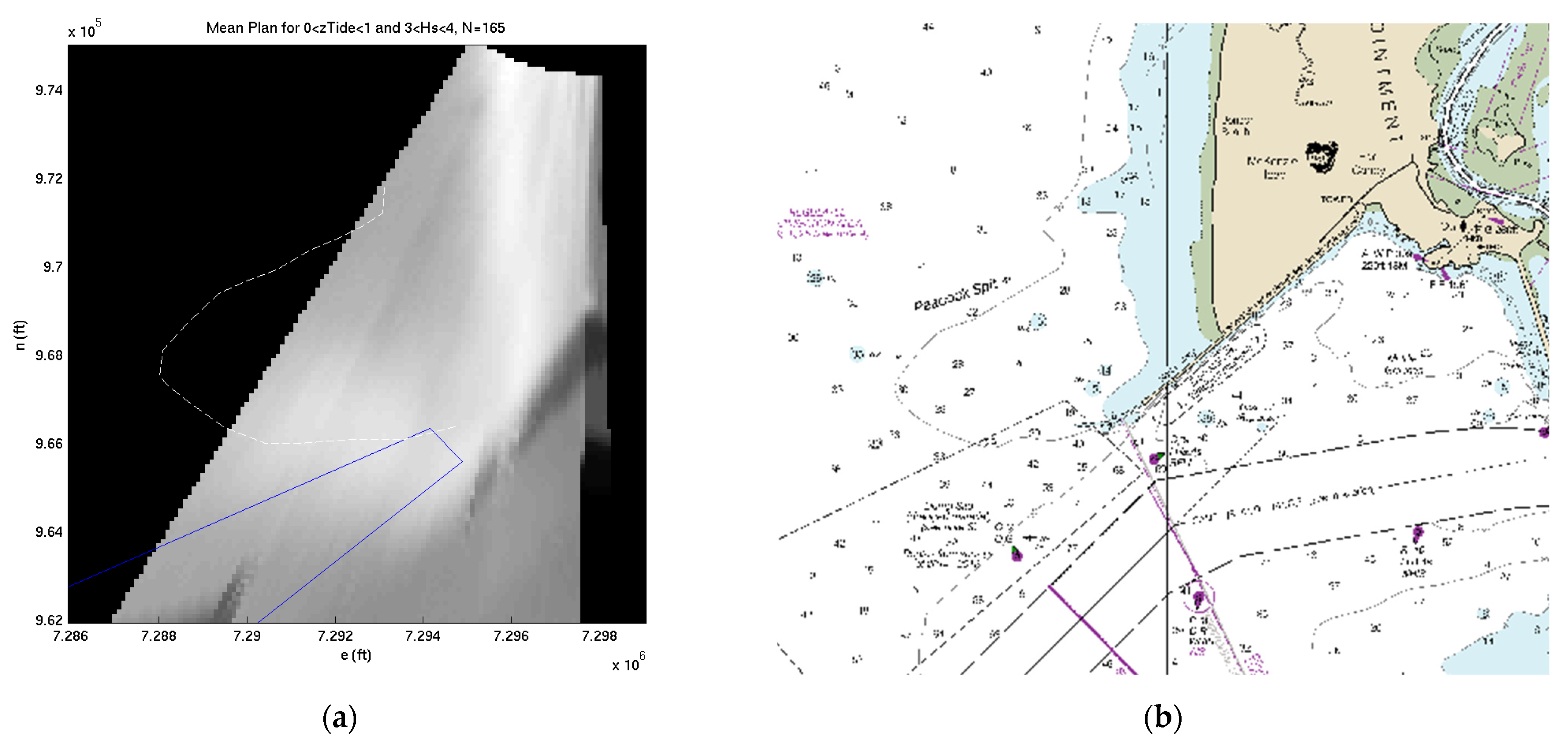
The north Columbia River jetty’s construction began in 1885. Due to the large viewing distances, only the north jetty is visible in the Argus data. Dredge material disposal for Columbia River sediments has been done at the “Shallow Water Site” (SWS) since 1973 in an attempt to keep sediments within the nearshore littoral system and available to the local beaches. The SWS site is located just to the north side of the navigation channel (location shown in Figure 4).

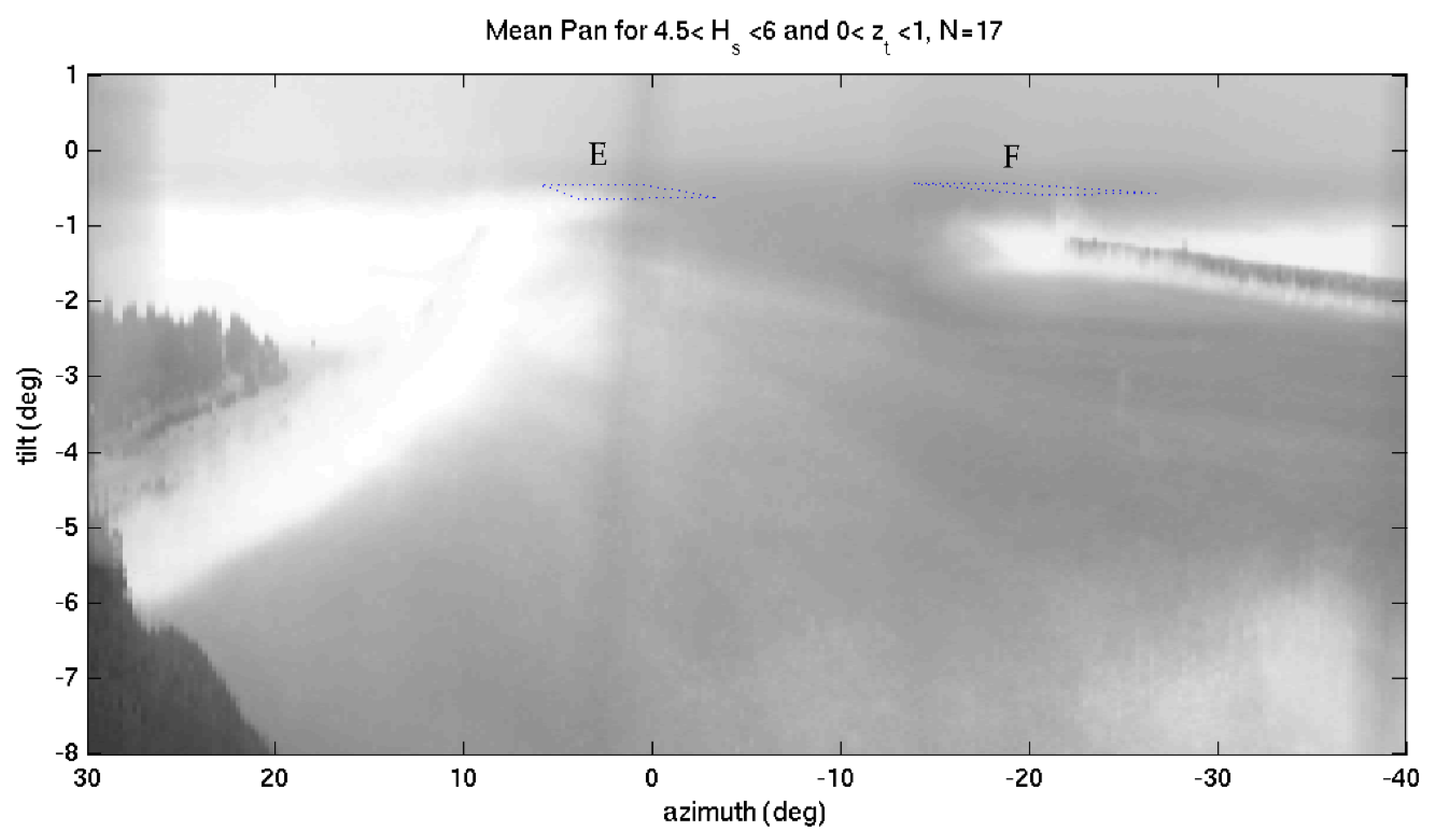
The Coos Bay jetties’ constructions began in 1890. Both jetties are visible in the Argus data, allowing measurement of wave breaking on both sides of the inlet. Coos Bay has two disposal sites: site E to the south of the offshore channel and site F to the north. Both locations are shown in Figures 6 and 12.

2.2. Argus Camera Sampling

Measurements were made from imagery collected by Argus stations at both sites. An Argus station is a set of cameras, computers, and software algorithms that have been developed and deployed since 1986 to take image data from which relevant nearshore measurements can be made [6].

For North Head, there was a requirement to sample with sufficient resolution out to a range of 4.5 km, the distance of the SWS disposal site from the North Head lighthouse. Due to the extreme range, five cameras were required to span the 40° field of view (Figure 1b) to allow sampling from Benson Beach on the left of the camera view out to the SWS location on the right. Each camera had a field of view of only 9.3° (50 mm lens) with a 5% overlap between adjacent images. 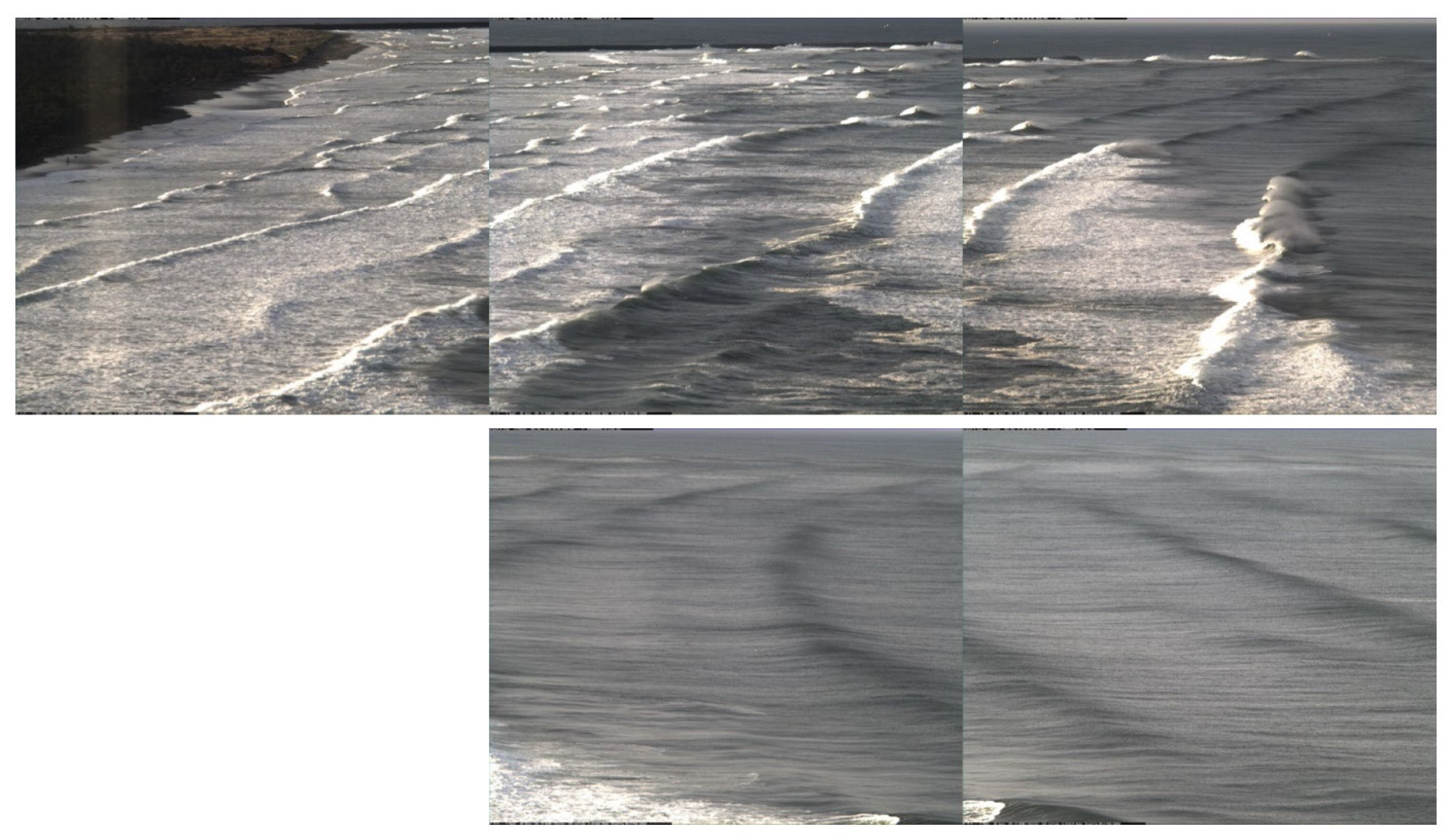Figure 2 shows example snapshot images from each camera.

To make geolocated measurements from imagery requires an understanding of photogrammetry, the quantitative transformation between image, and world locations of imaged features [7,8]. In general, this transformation between coordinates is accomplished through multiplication by the projective matrix, P. P contains information about the camera sensor, called the intrinsic calibration, which is performed once prior to camera installation, and information about the camera location and viewing angles, called the extrinsic calibration, that must be performed at installation and any time the camera moves. While camera location can be accurately measured at installation and will not change significantly, the viewing angles must be resolved to around 0.01° to maintain sufficient accuracy at the 3–4 km ranges of interest. For multi-year camera deployments like this, typical camera mounts are only stable to a factor of 10–100 times of this requirement, so quantification of the North Head image data required development of image co-registration algorithms. For the left-most camera, this process was based on the co-registration of land-based features, but for the right-most four cameras, registration was based on water-based features like details of breaker foam that were observable in the overlap regions between cameras, allowing the passing of geometry information from a camera on the left to adjacent cameras on the right. This development was challenging and important, but the details are beyond the scope of this manuscript (details will be featured in a future publication).

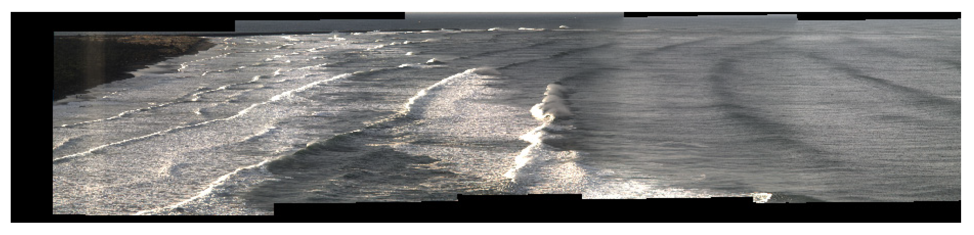
With photogrammetry accurately corrected, images from the five cameras could be merged into composite images in which world locations are accurately known. Figure 3 shows a merged panorama (pan for short) computed from the snapshot images in Figure 2. The pan axes are vertical and horizontal angles (tilt and azimuth) and world locations such as the SWS disposal site boundary can be accurately mapped in the composite image.

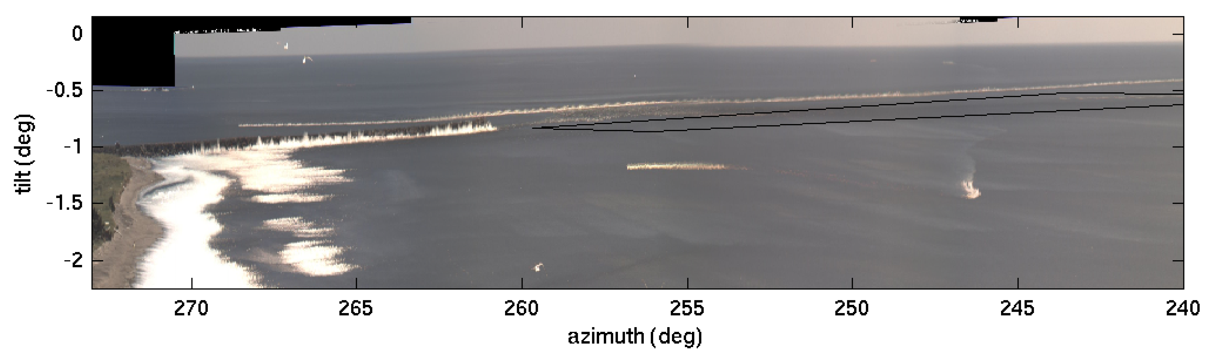
While snapshots provide an instantaneous feel for the wave conditions of the day, the goal of this paper is to estimate wave breaking statistics (defined below) on the jetty and at the SWS locations. Since wave heights modulate on several minute time scales, any particular snapshot can give a misleading representation of average breaking conditions. To improve our statistical representation of breaking, we use the “brightest” images [6]. For a “brightest” image, a series of snaps are taken at 2.0 Hz sampling frequency for ten minutes. The brightest intensity from those images for every pixel in the image is found and saved as a “brightest” image. 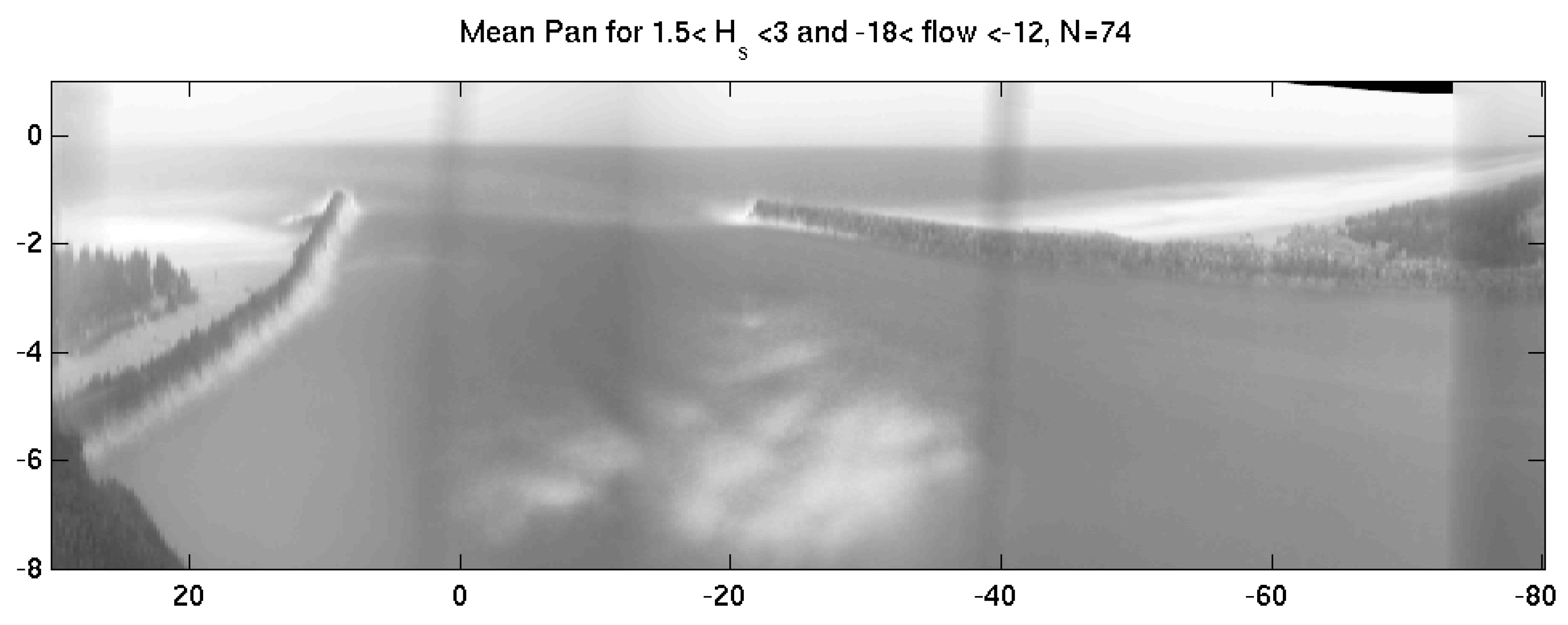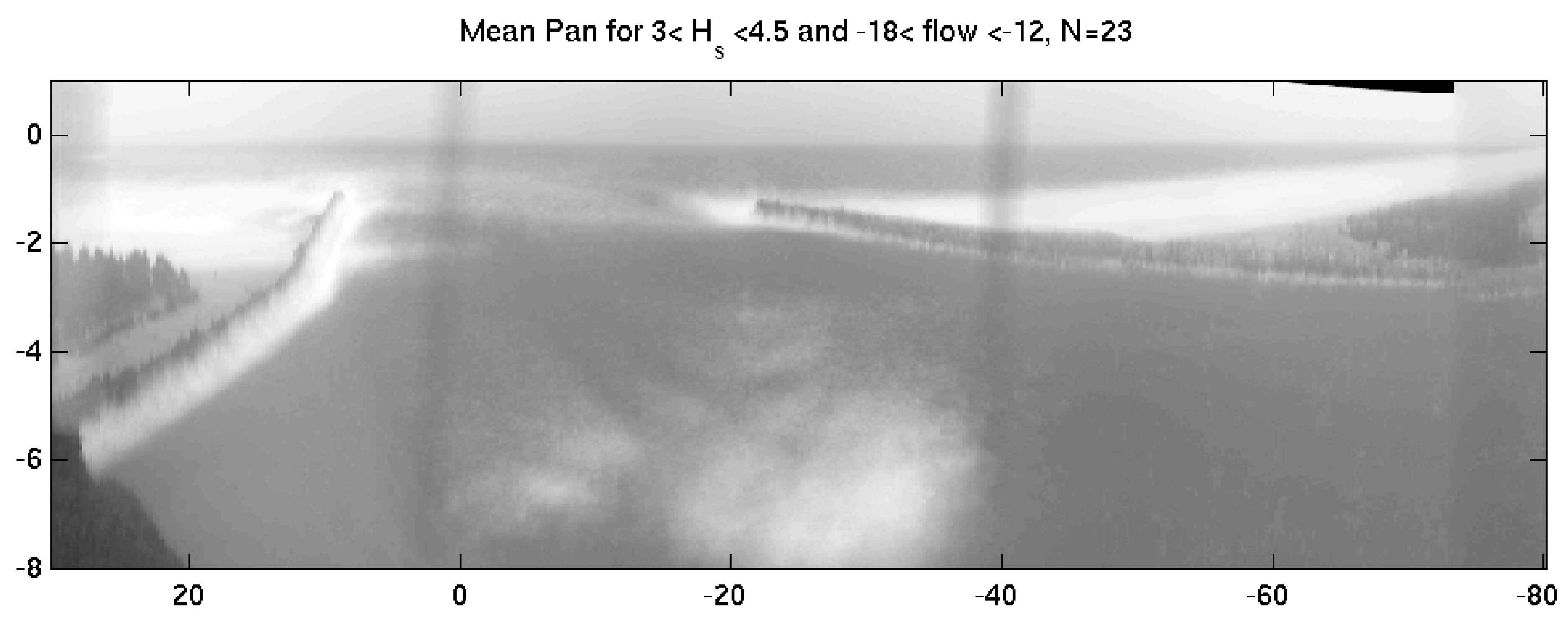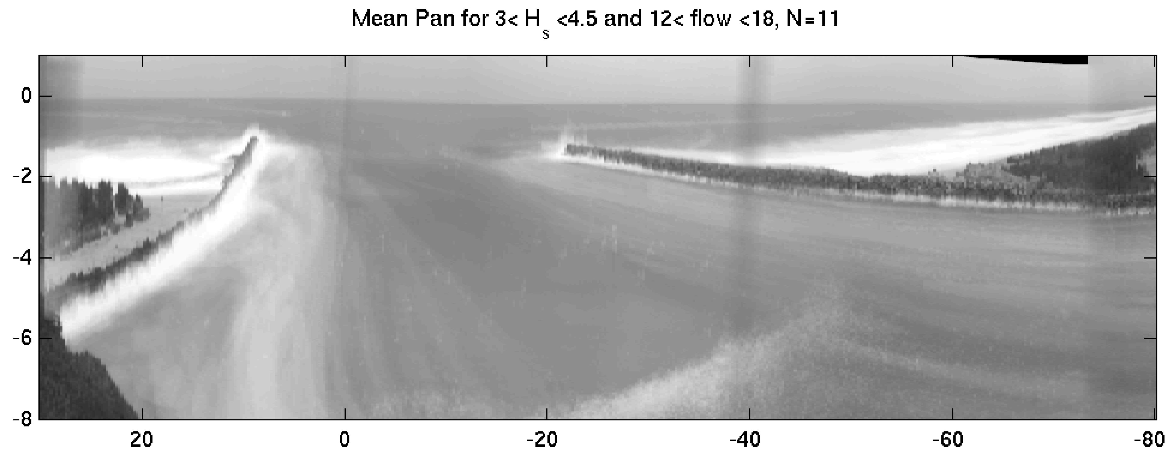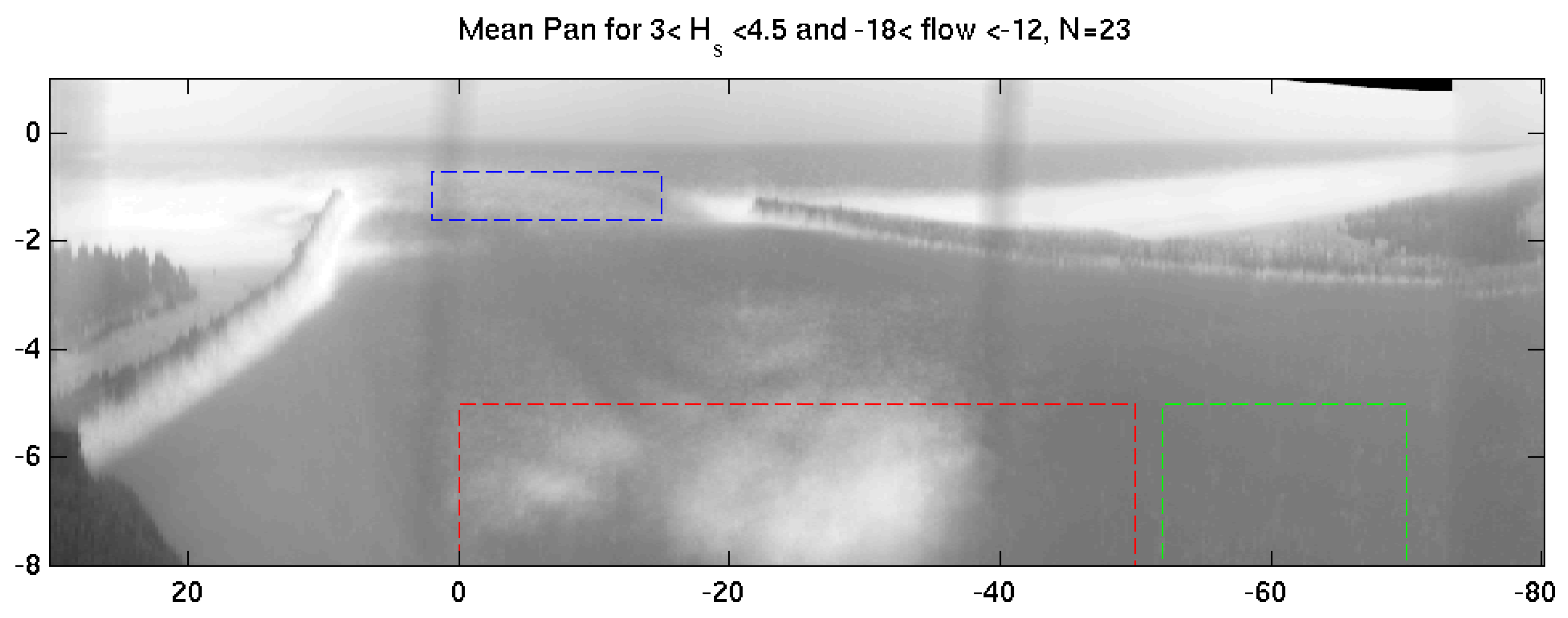Figure 4 shows an example of “brightest” panorama for 16 July 2017, a day with relatively low wave conditions. White areas indicate locations where wave breaking occurred at least once during the ten-minute collection, for example, along the shoreline and over a nearshore sand bar, as well as along the sides of the jetty. There are also some streak features due to boat wakes, for example, the long trail of a small boat entering the estuary just beyond the north jetty. The image shows azimuth and tilt angles for illustration. Images are shown with a vertical exaggeration of 4:1 to make features more visible. This has the effect of making breaking on the jetty look more extreme than it is. The boundaries of the SWS disposal site are included as a black line. The “brightest” images will be used to detect wave breaking on the north jetty and over the SWS disposal site.

The North Head Argus station ran from July 2017 to October 2019, for a total of 847 days. On each day, Argus images are collected every half hour for daylight hours, yielding a total of 13,009 image sets. Of these, many were unusable due to fog, rain, darkness, or sun glitter. These were removed by manually viewing every merged pan and flagging those that would be difficult or impossible to use. After manual culling, 5923 images remained, 45.5% of the total count.

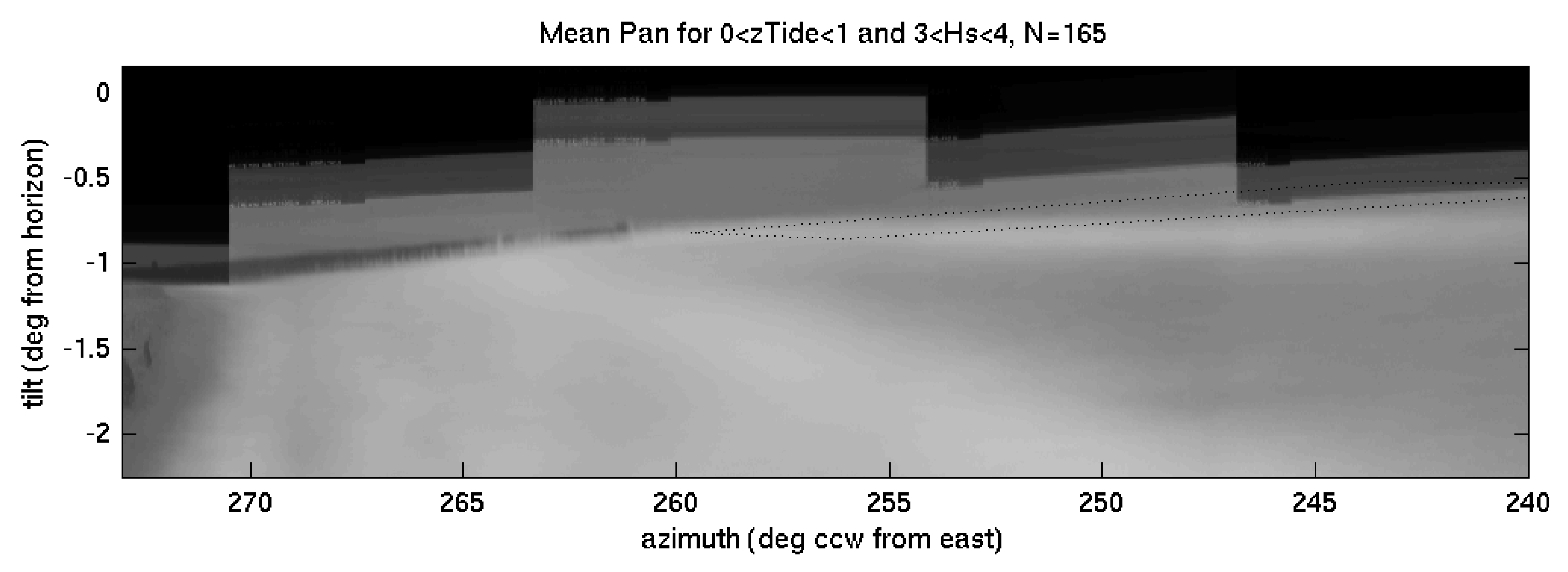
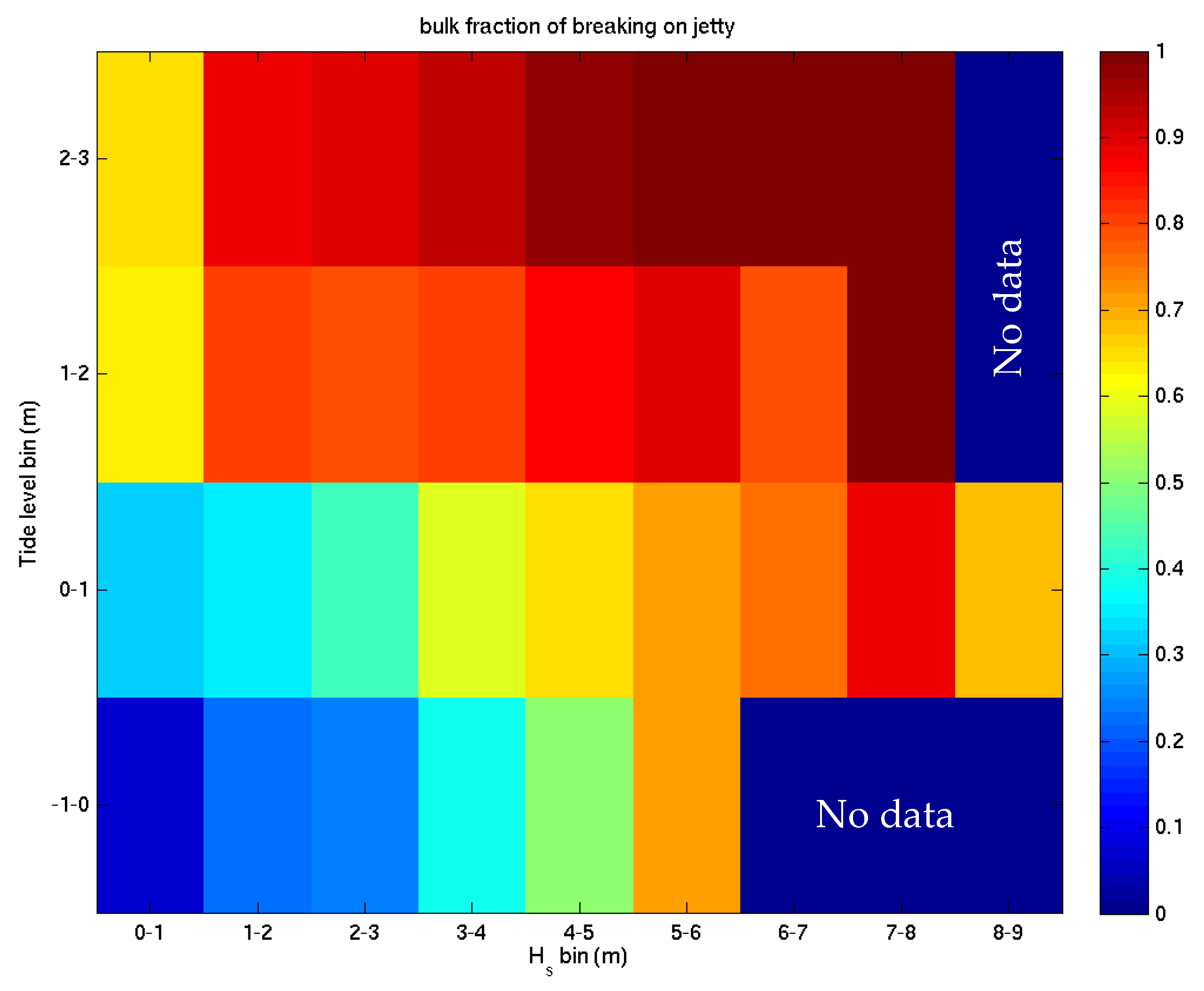
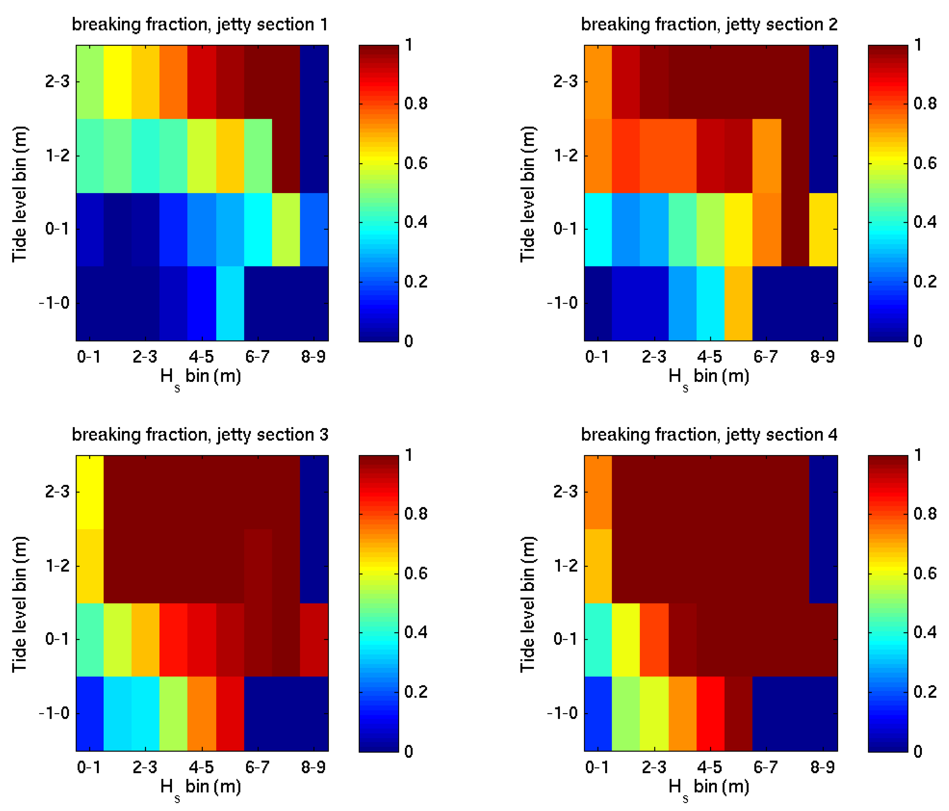
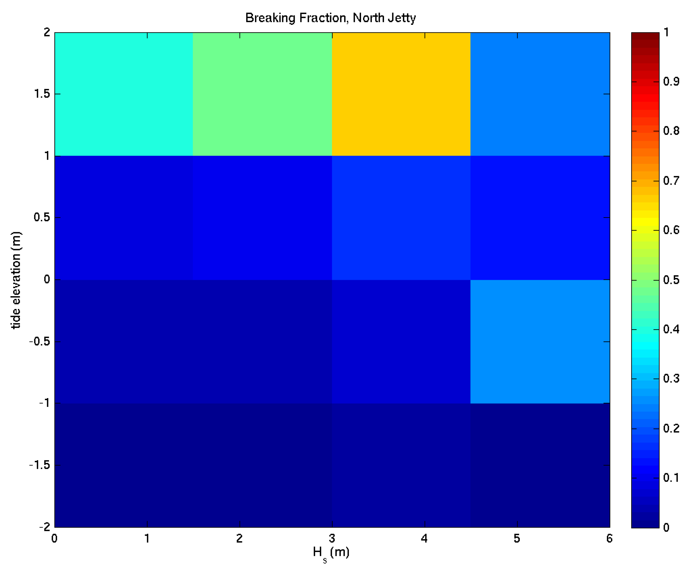
Wave breaking patterns depend on environmental conditions, mostly wave height and tide level. After viewing each of the almost 6000 pan images, it was clear that developing a robust quantification of the amount of breaking over the SWS disposal site and the north jetty was going to be challenging. Instead, it was decided to average all of the pans within each set of wave height and tide level bins. For North Head, the tide was partitioned into four elevation bins, −1 to 0, 0 to 1, 1 to 2, and 2 to 3 m. Significant wave heights, H_s, were partitioned into nine 1 m bins from 0 to 9 m. Thus, 36 averaged “brightest” pan images were computed. 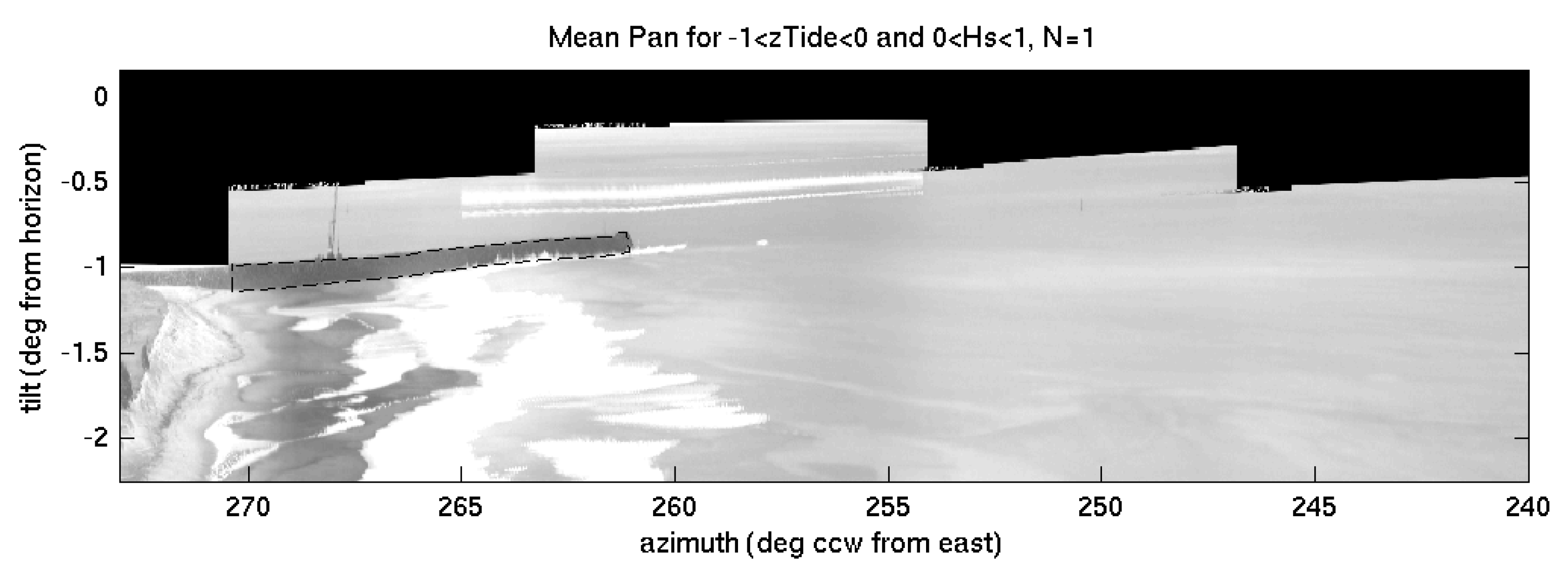Figure 5 shows a useful example of tide between 0 and 1 m elevation and H_s between 3 and 4 m. The number of individual pan images that contributed to the mean was also recorded, in this case 165. The upper limits of each image look like a double image. This is a consequence of the slow dipping of the camera tilt as the camera mounts aged over time. The fact that the jetty has a fixed location demonstrates the usefulness of the geometry correction process described above.

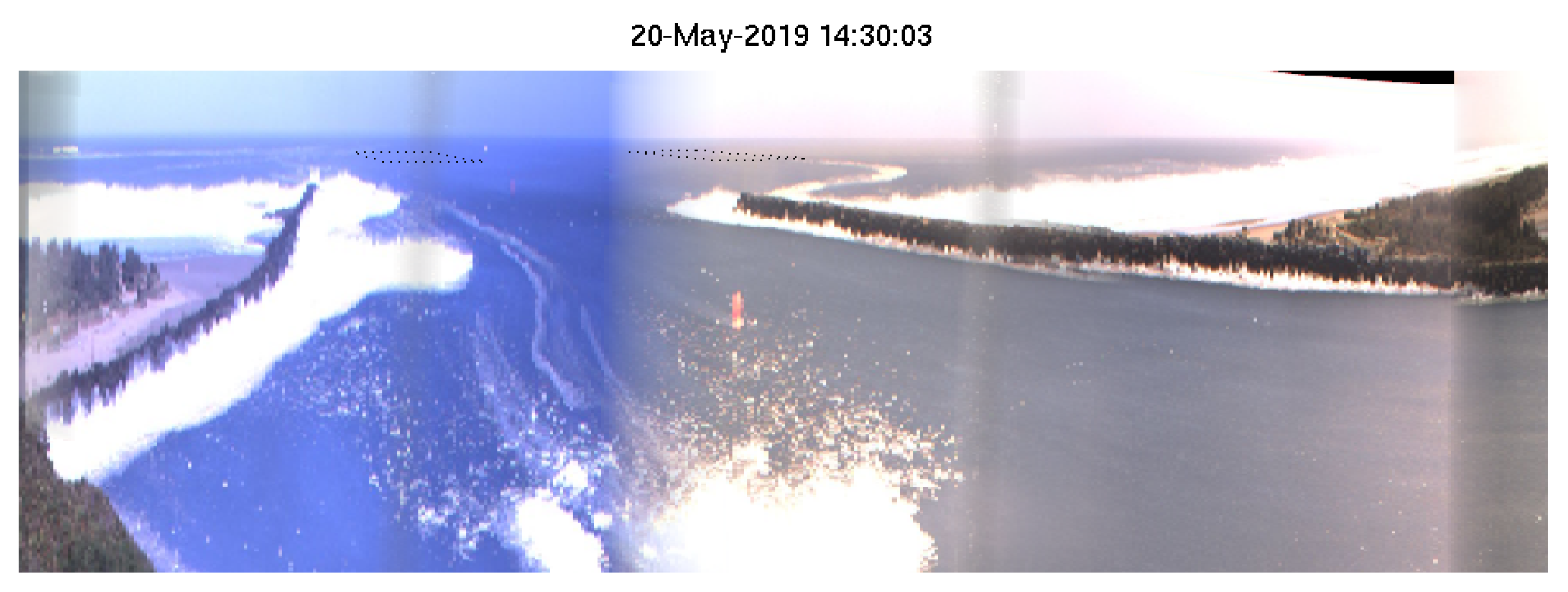
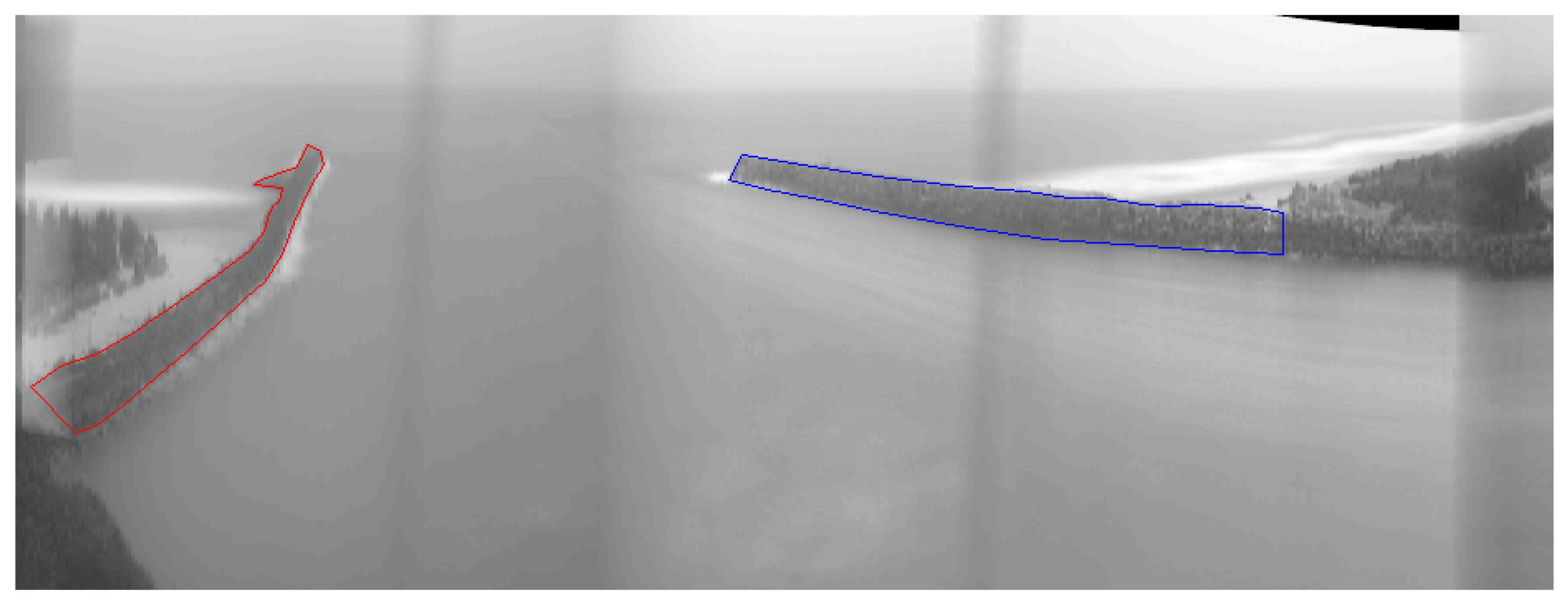
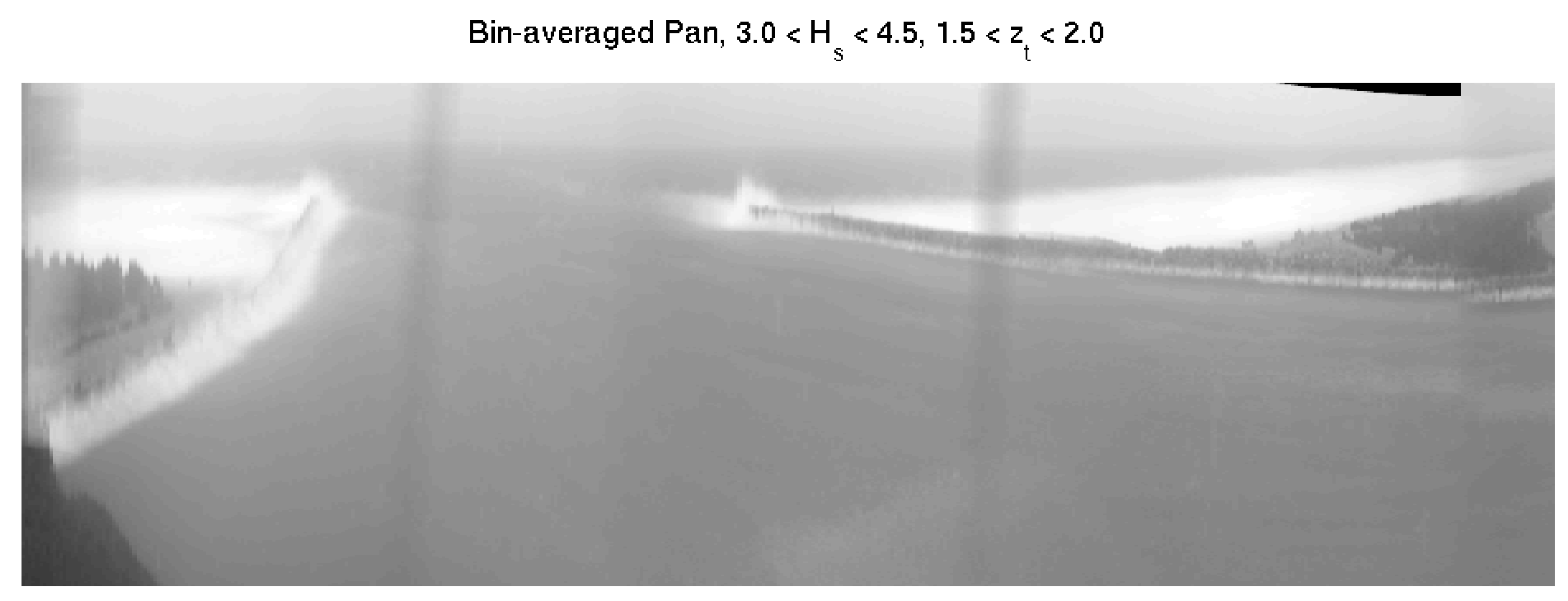
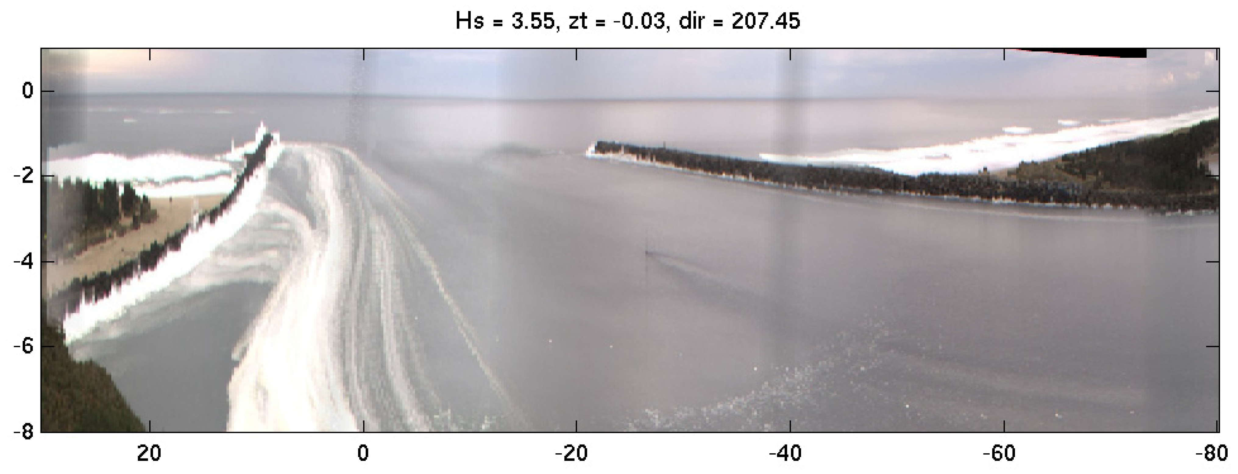
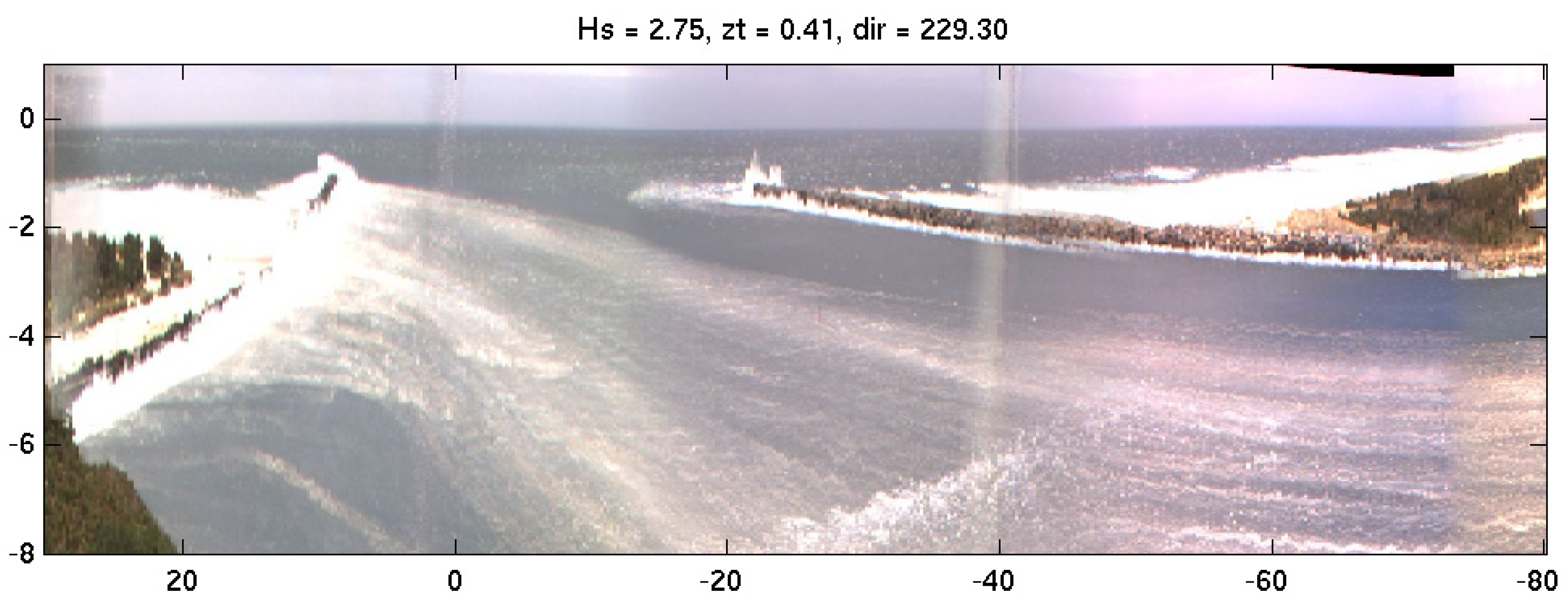
Most of the sampling for Coos Bay is similar to that for North Head. As seen in Figure 1c, six cameras were used to span almost 180° of viewing, including views back into the estuary. For this paper, we will only consider seaward looking views, so cameras 1 to 3. Figure 6 shows an example of “brightest” panorama from 20 May 2019, showing some wave breaking on both the north and south jetties as well as on the ocean beaches to the north and south. The boundaries of the two dredge disposal areas are shown offshore with dotted lines (site E is to the south or left, site F is to the north or right).

The Coos Bay site operated for a shorter time than North Head, running from 8 May to 27 November 2019, for a total of 202 days. In total, 6046 image sets were collected. Darkness, rain, and sun glitter made many of them unusable, but there were still 3122 good “brightest” pan images after culling.

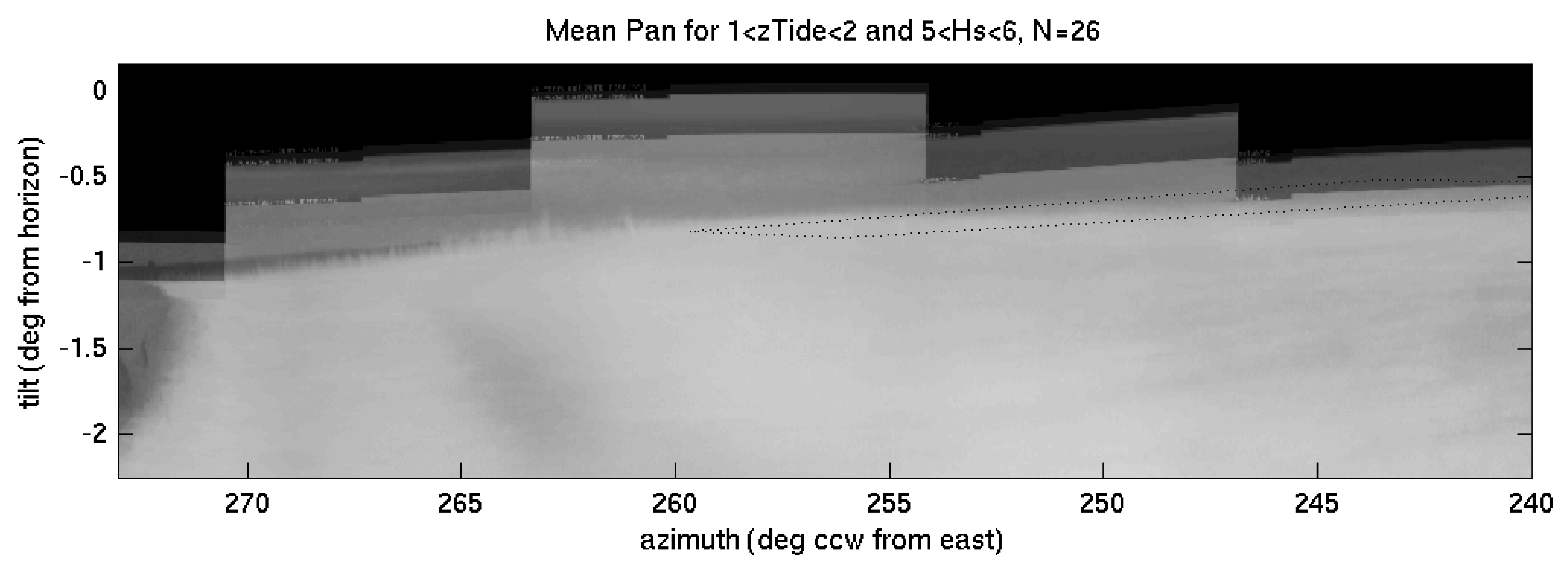
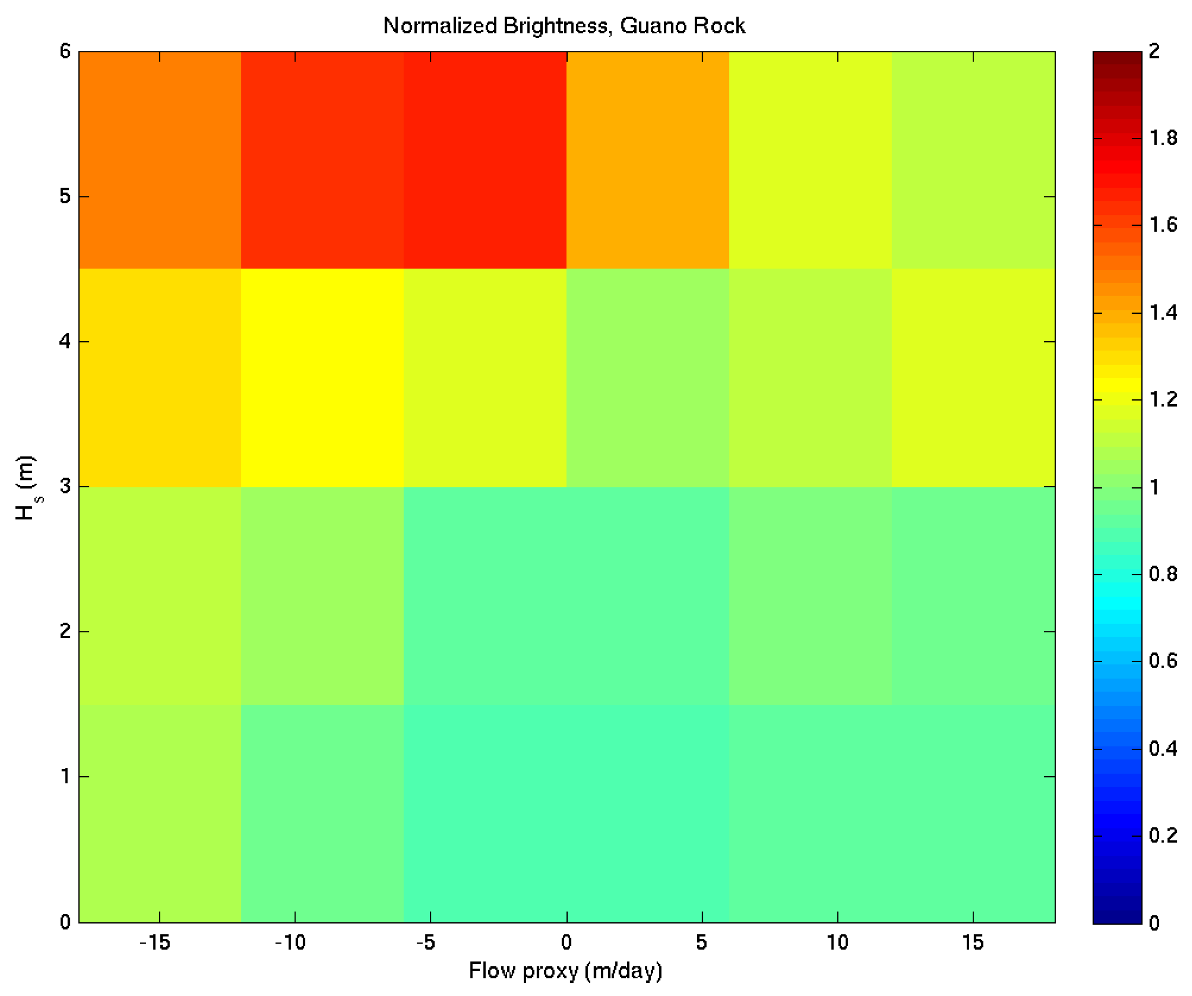
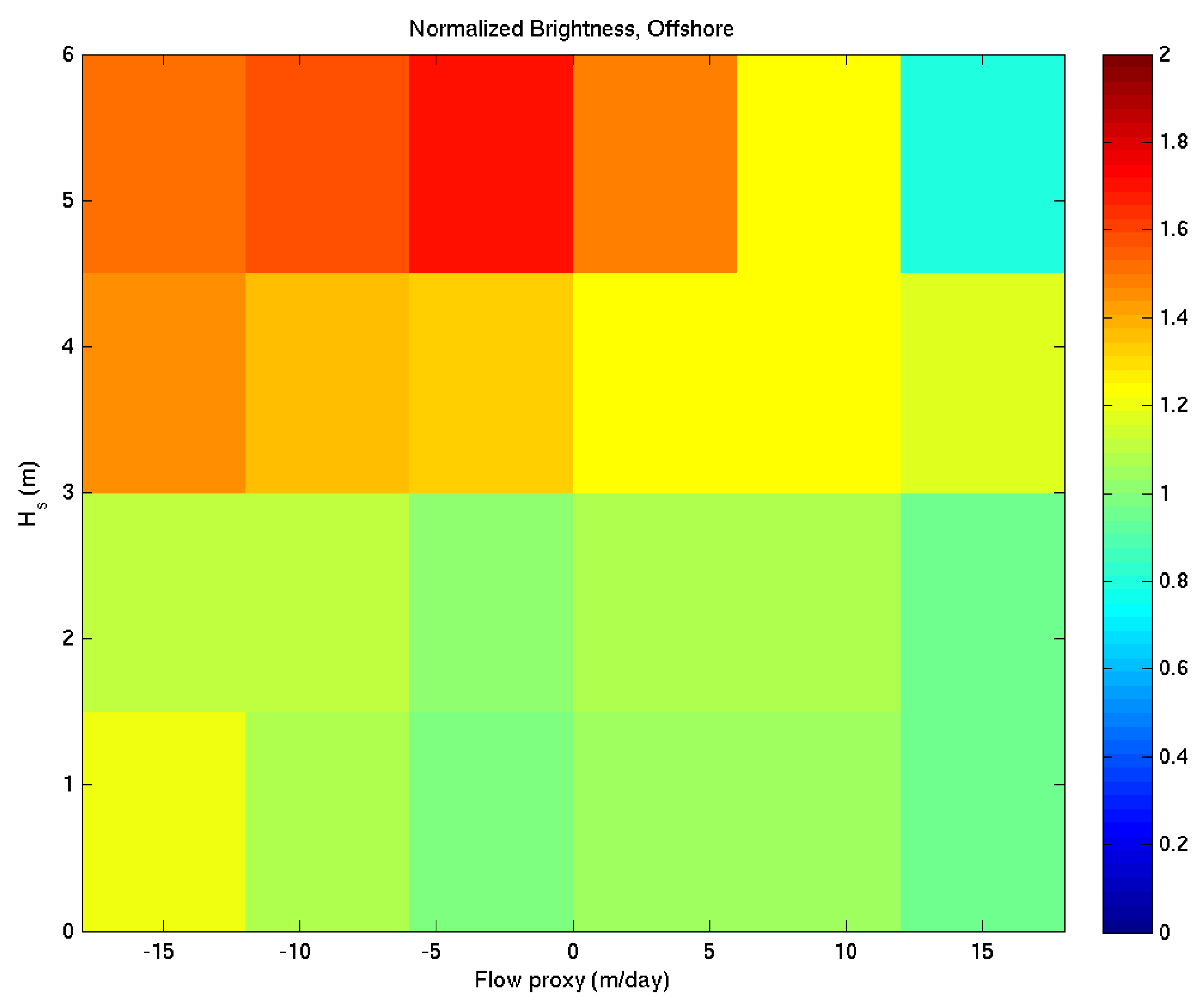
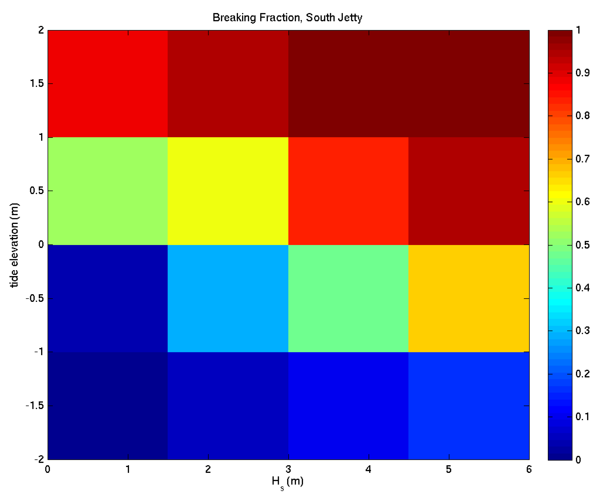
A similar bin-averaging was done for Coos Bay, although tidal flow was also felt to have an important influence on wave breaking patterns and was therefore included in the bin choices. For Coos Bay, significant wave heights, H_s, were partitioned into four bins from 0 to 6 m with bin size of 1.5 m. Tide elevation was split into four bins, from −2 to +2 m with 1 m bin sizes. There were no direct estimates of tidal flow, so the finite difference of tidal elevation (dz_t/dt) was used as a tidal flow proxy (t measured in days). Tidal flow was partitioned into 6 bins, from −18 (spring ebb) to +18 (spring flood) with bin sizes of 6 m/day (this is not a horizontal flow, but instead is a rate of tidal elevation change).

3. Results

The following sections document the main results regarding wave breaking over the disposal sites and jetties for each of the two locations.

3.1. North Head

One of the main purposes of the North Head sampling was to determine if the SWS dredge disposal site caused enhanced wave breaking that would be a hazard to navigation. Thus, “brightest” images were an excellent tool to assess this problem. Figure 5 shows an example of bin-averaged “brightest” pan for tide elevations between 0 and 1 m and wave heights between 3 and 4 m, averaging a total of 165 images within this bin. There is a clear concentration of breaking seaward of the jetty in a white band that extends offshore from the jetty tip. An examination of the full set of bin-average pans showed that this anomalous band was not visible for wave heights of less than 2.0 m but was then a consistent feature up to wave height around 5 m after which surf zone breaking appeared to be broadly saturated (Figure 7). Little dependence on tide elevation was seen.

Both Figure 5 and Figure 7 also show the boundaries of the SWS disposal site as a dotted line. After close examination, it was clear that for all bin-averaged brightest pans, the region of enhanced breaking was oriented and located northward of the SWS boundary (closer to the camera). This is more evident if the pan image from Figure 5 is reprojected to a map view; Figure 8a. The band of white breaking is seen to extend mostly to the west northwest, not following the SWS boundaries shown in blue. Instead, the region of enhanced breaking appears to be following the flank of a shoal called Peacock Spit, shown in the nautical chart in Figure 8b and repeated as a white dashed line in the map view in Figure 8a. There is no evidence from any of the brightest images that the SWS disposal site was causing enhanced breaking or a hazard to navigation.

The brightest pans in Figure 4, Figure 5 and Figure 7 all show evidence of wave breaking on the north jetty (this is vivid in Figure 4 but more averaged out in Figure 5 and Figure 7). Since wave breaking is a primary stress on jetty structure, it was decided to use these images to quantify the extent and environmental dependencies of this breaking. The jetty region was digitized using the bin-averaged pan with the lowest tide and wave heights, z_t < 0 m, H_s < 1 m, of which there was only one case (Figure 9, the blue dashed line defines the jetty region). For each of the remaining 35 bin-averaged pans, the fraction of this region that was obscured by breaking waves (brightness exceeding a threshold intensity selected manually by viewing intensity histograms) was recorded. Figure 10 shows the resulting bulk breaking fractions as a function of wave height and tide elevation. Not surprisingly, higher tides yield more breaking over the jetty. Increasing wave heights also increases the breaking fraction substantially until it reaches essentially 100% for storms at mid to high tides.

Breaking percentage varies with distance along the jetty. To quantify this, the jetty region was broken up into four quarters, from landward to seaward, and the fraction of breaking was found in each section (Figure 11). It is clear that the outer half of the jetty experiences significant breaking regularly for wave heights > 1 m and mid to high tides. The inner half of the jetty is better protected, except during high tides.

3.2. Coos Bay

As with North Head, our main sampling purposes at Coos Bay were to determine whether the offshore dredge disposal sites caused enhanced breaking and hence acted as a hazard to navigation, and to characterize wave breaking on the two jetties. These tasks were accomplished using bin-averaged “brightest” panoramas.

Mean pan images were computed for bins comparing H_s, the significant wave height, with z_t, the tide elevation (this was a four-by-four suite of panBars). Figure 12 shows an example for the largest wave heights, H_s > 4.5 m, and mid to high tides (an average of 17 cases, the best example for the largest waves). As can be seen from the dotted lines outlining the two dredge disposal regions, there is no breaking in Site F, to the north, and only a tiny overlap of breaking with Site E, to the south. In fact, this minor overlap is only due to the overlay problem, whereby the tops of waves breaking at landward locations are mapped to a further offshore location in the rectification process (the same effect that causes the north jetty to stretch north in Figure 8). To ensure this conclusion, every “brightest” pan for which wave heights were greater than 4.0 m was examined manually. A total of 90% showed no overlap at all of breaking with Site E, while 10% showed slight overlap of the southeastern tip of the disposal site due to the overlay problem. It can be safely concluded that these two disposal sites had no impact on wave breaking for the 202 days that were sampled and do not cause enhanced wave breaking that could be a hazard to navigation.

Wave breaking within and just offshore of the inlet can also present as hazards to navigation and is expected to depend on both the offshore wave height and the tidal flow, here represented by the tidal flow proxy dz_t/dt. As indicated earlier, tidal flow was divided into six proxy bins, from −18 by 6 to +18. These can be thought of as spring ebb, normal ebb, weak ebb for negative values, and the same for flood as positive values.

Figure 13 shows an example of breaking over Guano Rock, in the south center of the jettied channel, for low-to-moderate wave heights and spring ebb flows. There is a clear region of wave breaking near the camera, due to the strong ebb flows causing breaking over Guano Rock (note that this is well south of the main channel, which is on the right looking out). There is also a slight increase in breaking at the mouth of the inlet (between and seaward of the jetty tips) as incoming waves encounter the opposing ebb flows.

Figure 14 shows the same pattern, but a bit exaggerated, for larger waves between 3.0 and 4.5 m in height. In this case, the inlet breaking is more obvious. It is surprising how well the details of breaking over the Guano Rock region are replicated. Finally, Figure 15 shows the mean “brightest” image for moderate-to-large wave height and maximum flood flows. There is no longer enhanced breaking at the mouth of the inlet. The breaking over Guano Rock is now shifted landward by the flood flows and is much more linear in an across-channel direction.

Both wave height and tidal flow seem to play a role in these breaking patterns. To explore this more systematically, the 24 bin-averaged pan images (six flow bins by four wave height bins) were computed and the mean intensities were measured in three regions, Guano Rock, the mouth of the inlet between the jetties (called Offshore), and a mid-channel region away from Guano Rock that could act as an intensity normalization (Figure 16).

Mean intensities were found for each H_s-flow combination for the Guano Rock and offshore regions, and were then normalized by the intensity from the normalization region. The results for Guano Rock are shown in Figure 17. Breaking over this feature increases with wave height, with some breaking for most cases of wave heights greater than 3 m. However, breaking is also clearly dependent on tidal flow, being weakest at low flows and stronger in ebb flows (negative) than in floods. For the largest waves, breaking is persistent, although much less during flood flows. Note that for the highest wave bin, there are only one and two cases for the extreme flows, so statistics are expected to be noisy.

Figure 18 shows a companion figure for the offshore sampling region. Again, breaking between the jetties increases with wave height, but it also shows the weak but expected asymmetry with enhanced signals for strong ebb flows and no enhancement during floods.

As with North Head, the “brightest” pan images have clear signatures of wave breaking around and over the jetties (e.g., Figure 12). The regions of interest (ROIs) were defined for both the north (blue line) and south (red line) jetties by manual digitization of the breaker footprint in a bin-average “brightest” pan that had the lowest wave heights and the lowest tides (Figure 19, which averaged 96 individual pans). Thereafter, for each wave-height tide bin, the fraction of pixels within each ROI whose brightness exceeded a breaking brightness threshold were determined as the breaking fraction for that bin.

Figure 20 shows the breaking fraction statistics for the north jetty. Only one bin shows breaking fractions greater than 0.5 with a mean over all bins of 0.17. These low values likely reflect the fact that we are seeing the inner, protected face of the jetty and that the south jetty extends further seaward, perhaps providing extra protection. In contrast, breaking fractions for the south jetty are much larger (Figure 21). Just over half of the bins had breaking fractions that exceed 0.5, and the mean value over all bins was 0.53. The viewing angle of the south jetty is primarily from the top rather than from the protected inner side. Despite this geometric aspect, it is clear that the south jetty experiences much greater wave breaking energy than the north.

Several other interesting features can be observed in the brightest images. While the north jetty does not show much breaking, breaking at the jetty tip can be dramatic, especially for high tides. Figure 22 shows breaking at the tip of the north jetty for the bin-averaged pan for medium to high waves (3.0 < H_s < 4.5) and high tides (1.5 < z_t < 2.0). The height of the jetty top and splash were roughly digitized, and the splash was found to be roughly 3.28 times as high as the jetty (2.28 exceedance of jetty top height). A scan of the top several hundred individual pan images with higher tide and at least 2.0 m of wave height showed that most of the intense breaking on the north jetty is focused on the seaward 100 m.

Finally, anomalous behavior was sometimes noted along the south jetty when wave energy was strong from the south. In Figure 14 and in many others, we noticed an apparent wave dissipation feature on the north side of the south jetty, roughly aligned with the south beach shoreline. Looking over pans, we noticed that the south jetty looked “leaky” at this location at times, perhaps allowing sediment to pass through under conditions of strong southerly waves. Figure 23 shows one example with medium to large waves (Hs = 3.55 m) arrived from the south (wave direction 207°, shore normal is 300°). Foam is being carried from the tip of the south jetty into the inlet by the flood tide. However, there is also a source of foam midway along the north side of the south jetty, in the region of the breaking anomaly that was referred to above. This is at low tide and the jetty is not being overtopped.

Figure 24 provides another example. In this case, the jetty appears to be overtopping in the near beach region (but not further seaward). We are not sure if this is a low point in the jetty. Again, the waves are approaching from the south (direction = 229°, shore normal of 300°) and foam is being carried landward by the flooding tide. It should be noted that these observations of potential jetty leaking of the south jetty are very preliminary.

4. Discussion

To the authors’ knowledge, this is the first use of “brightest” images to study wave stresses on engineering structures. These camera-based data collections appear to be an excellent method to detect and characterize wave breaking. The camera systems are cheap and can be programmed to collect data each half hour for years. Photogrammetry is now well understood and allows mapping of potential hazard areas such as dredge disposal sites. With such systems, it is easy and cheap to collect many thousands of images for analysis. Bin-averaged images allow for statistically robust characterizations of breaking patterns on jetties, including conclusions, for example, about the relative wave breaking probabilities on the north versus south Coos Bay jetties and the detection of an apparent jetty low point midway along the south jetty.

“Brightest” images detect the presence of any breaking during the 10-min data collection and do not distinguish whether a single or many waves broke. If only one wave broke, this would be equivalent to roughly a 1% exceedance statistic for an example of 6-s waves (one out of 100 waves). In other words, regions with no indication of breaking in a “brightest” image are more than 99% likely to have no breaking. This is a good first step to characterizing the breaking waves and simply partition a region like a jetty into breaking and non-breaking sections. But there may be several options if more average statistics are desired. The easiest would be to use time-exposure images from the same 10-min collection period. This would require some study of the sensitivity of the resulting gradations of value to the actual frequency of wave breaking. An unusual alternate might be to use individual frames from “wave-averaged movies” (WAMs; [9]). Each frame of a WAM is the average of typically 20 s of 2 Hz frames, long enough to average out the individual waves, but short enough to detect motion in currents (their main use) or fluctuations in whether waves broke in that period or not. Such a method would need study.

Data from North Head spanned 847 days, so more than two years. On the other hand, Coos Bay only ran for 202 days and had no data collections during the most energetic winter months. Thus, breaking statistics for Coos Bay do not represent the full storm energy being experienced by the jetties and more data would be useful.

Finally, there were some aspects of the observations that seem particularly interesting and deserve further investigation. Most notably, the middle section of the south jetty at Coos Bay appears to experience overtopping more than any other section, perhaps due to a lower elevation. In addition, there are indications of sand leaking through at this location that would be important to further nail down. On the north side, most of the breaking was concentrated on the seaward-most 100 m or so of the jetty and included very large breaking and spray events that deserve further study.

5. Conclusions

Argus optical imaging methods were used to study wave breaking characteristics at two high-energy PNW inlets, the very large Columbia River inlet between Washington and Oregon states, and the smaller inlet at Coos Bay to the south. In both cases, the goals were twofold; to test whether nearshore dredge disposal sites caused enhanced wave breaking that could be a hazard to navigation, and to examine the statistics of wave breaking over inlet jetties. For the Columbia River, the Argus station was located in the North Head lighthouse, 3 km to the north of the north jetty, and ran for 847 days from 2017–2019. For Coos Bay, the station was located at a coast guard watch station with a good view of both jetties and two offshore disposal sites and ran for 202 days in 2019.

“Brightest” images were used for breaker detection since these images capture the brightest each pixel gets during a 10-min data collection, and brightness is clearly dominated by wave breaking. The roughly 6000 resulting good-quality image sets from North Head and 3000 from Coos Bay showed breaking patterns that varied with the wave and tide conditions. To capture these dependencies, images were averaged into a set of bin partitions of wave height, tidal elevation, and tidal flow, and conclusions were drawn strictly from these bin-averaged results.

For both sites, there was no indication of enhanced wave breaking over the nearshore dredge disposal sites for even the largest waves and the lowest tides. A band of enhanced breaking was seen to extend seaward from the Columbia River north jetty for wave heights greater that 2 m, but the band follows the flanks of Peacock Spit, a natural shoal, and is well north of the disposal region. For Coos Bay, there was no significant breaking over the two disposal sites but wave breaking in the inlet mouth was clearly enhanced under ebb flow conditions. Overall, there is no evidence that these dredge disposal sites are a hazard to navigation.

Wave breaking over the Columbia River north jetty reaches 100% (at least one breaker in each 10-min sampling period) for the seaward half of the jetty when wave heights exceed 3 m at mid tide or higher. For Coos Bay, the south jetty sees much more wave breaking than the north, with high levels of jetty breaking at mid to high tides and wave heights greater than 2 m. Surprisingly, the mid jetty region sees more overtopping that the seaward tip and appears to leak sediment from the adjacent beach into the inlet.

References

1. Moritz, H.R.; Gelfenbaum, G.R.; Kaminsky, G.M.; Ruggiero, P.; Oltman-Shay, J.; Mckillip, D.J. Implementing Regional Sediment Management to Sustain Navigation at an Energetic Tidal Inlet. In Coastal Sediments 07; ASCE: New Orleans, LA, USA, 2007. [Google Scholar]
2. USACE. Major Rehabilitation Evaluation of the Jetty System at the Mouth of the Columbia River, OR and WA, Oregon/Washington; P.D.a.U.S.E.P.A. U.S. Army Corps of Engineers, Region 10, Editor. 2012: Portland Oregon and Seattle Washington. Available online: https://usace.contentdm.oclc.org/digital/collection/p16021coll7/id/9859/ (accessed on 11 June 2022).
3. USACE/USEPA. 2021 Annual Use Plan, Management of Open Water Dredged Material Placement/Disposal Sites Mouth of the Columbia River, OR and WA, Oregon/Washington; P.D. US Army Corps of Engineers, and US Environmental Protection Agency: Portland, OR, USA; Seattle, WA, USA, 2021.
4. Komar, P.D.; Allan, J.C.; Ruggiero, P. U.S. Pacific Northwest Coastal Hazards: Tectonic and Climate Controls. In Coastal Hazards; Finkl, C.W., Ed.; Springer: Dordrecht, The Netherlands, 2013; pp. 587–674. [Google Scholar] [CrossRef]
5. Ruggiero, P.; Komar, P.D.; Allan, J.C. Increasing wave heights and extreme value projections: The wave climate of the U.S. Pacific Northwest. Coast. Eng. 2010, 57, 539–552. [Google Scholar] [CrossRef]
6. Holman, R.A.; Stanley, J. The history and technical capabilities of Argus. Coast. Eng. 2007, 54, 477–491. [Google Scholar] [CrossRef]
7. Hartley, R.; Zisserman, A. Multiple View Geometry in Computer Vision, 2nd ed.; Cambridge University Press: Cambridge, UK, 2004. [Google Scholar] [CrossRef] [Green Version]
8. Holland, K.T.; Holman, R.A.; Lippmann, T.C.; Stanley, J.; Plant, N. Practical use of video imagery in nearshore oceanographic field studies. IEEE J. Ocean. Eng. 1997, 22, 81–92. [Google Scholar] [CrossRef]
9. Anderson, D.; Bak, A.S.; Brodie, K.L.; Cohn, N.; Holman, R.A.; Stanley, J. Quantifying Optically Derived Two-Dimensional Wave-Averaged Currents in the Surf Zone. Remote Sens. 2021, 13, 690. [Google Scholar] [CrossRef]
Figure 2. Example snapshots from each of the five cameras from North Head for 12 March 2018, 1530 GMT.
Jmse 10 01037 g002
Figure 3. Panoramic view merging the five snapshots in Figure 2.
Jmse 10 01037 g003
Figure 4. Example of merged pan “brightest” image from 16 July 2017 showing regions of wave breaking during the ten minutes of data collection, for example, over the shoreline and sand bar and against the jetty. Anomalous streaks correspond to boat wakes. The SWS boundaries are shown offshore as a black line. The figure is shown with a vertical exaggeration of 4:1 to improve interpretation.
Jmse 10 01037 g004
Figure 5. Example of averaged pan “brightest” image for North Head for the 165 images for which the tide elevation was between 0 and 1 m and the wave height was between 3 and 4 m. The SWS disposal site is shown by the black dotted lines extending from the end of the jetty.
Jmse 10 01037 g005
Figure 6. Example of pan “brightest” image of the seaward region of interest (ROI) for Coos Bay for 20 May 2019, 1430 GMT. The wave height was 2.35 m, period was 11.0 s, tide level was −1.63 m and the wave direction was 252°. The Site E and Site F dredge disposal sites are marked offshore of the inlet with lightly dotted lines. A red channel marker is visible near the inlet center. The white region at the bottom of the image corresponds to wave breaking over Guano Rock, a submerged feature (the main channel lies to the right of this location).
Jmse 10 01037 g006
Figure 7. Example of averaged pan “brightest” image for the 26 images for which the tide elevation was between 1 and 2 m and the wave height was between 5 and 6 m. Breaking for very large wave heights appears to saturate across the full surf zone.
Jmse 10 01037 g007
Figure 8. (a) Rectified (map) North Head re-projection of the panoramic view in Figure 5 onto Oregon state plane coordinates. The jetty is visible angling to the southwest. The SWS boundary is shown by the blue line and lies to the southwest of the band of enhanced wave breaking. (b) Nautical chart of the same region showing Peacock Spit on the north side of the jetty. The Peacock Spit boundary is reproduced in (a) and corresponds to the region of enhanced breaking.
Jmse 10 01037 g008
Figure 9. Averaged pan image for the lowest tides and lowest waves (only one image fit this condition). The jetty was manually digitized (dashed blue line) to define the region of interest for breaking detection. This region was then applied to pan images for all tide and wave height bins to detect the fraction that was obscured by breaking waves.
Jmse 10 01037 g009
Figure 10. Bulk fraction of breaking over the jetty region as a function of significant wave height (x-axis) and tide elevation (y-axis). Blue regions at very large wave heights are due to there being no examples in these bins.
Jmse 10 01037 g010
Figure 11. Fraction of breaking on the jetty, partitioned by jetty section from Section 1 (most landward, top left) to Section 4 (most seaward, bottom right). Zero values at large wave height correspond to there being no cases at those conditions.
Jmse 10 01037 g011
Figure 12. Bin-averaged “brightest” pan for wave heights greater than 4.5 m and mid to high tides. A total of 17 individual pans were included in this average. The E and F dredge disposal sites are shown with dotted lines.
Jmse 10 01037 g012
Figure 13. Bin-averaged “brightest” pan for wave heights between 1.5 and 3.0 m and spring ebb flows. The strong ebb flows cause breaking over Guano Rock (lower center of the image), as well as a slight increase in breaking at the mouth of the inlet.
Jmse 10 01037 g013
Figure 14. Bin-averaged “brightest” pan for wave heights between 3.0 and 4.5 m and spring ebb flows. The enhanced breaking over Guano Rock continues but the breaking at the mouth of the inlet is more evident.
Jmse 10 01037 g014
Figure 15. Bin-averaged “brightest” pan for wave heights between 3.0 and 4.5 m and spring flood flows. There is no longer any enhanced breaking in the inlet mouth and the breaking over Guano Rock is shifted landward by the flood flow in a more cross-channel linear direction.
Jmse 10 01037 g015
Figure 16. Mean intensity sampling regions. Red is the region of Guano Rock, blue shows the Offshore region, and green shows the intensity normalization region.
Jmse 10 01037 g016
Figure 17. Normalized brightness of Guano Rock sampling region as a function of wave height and tidal flow (proxy).
Jmse 10 01037 g017
Figure 18. Normalized brightness of offshore sampling region as a function of wave height and tidal flow (proxy).
Jmse 10 01037 g018
Figure 19. Regions of interest (ROIs) for wave breaking over the Coos Bay jetties with the north jetty ROI marked in blue and the south in red. The regions were manually delineated using this bin-averaged pan for the smallest wave height and lowest tide bin that averages 96 cases.
Jmse 10 01037 g019
Figure 20. Breaking fraction statistics for the north jetty as a function of wave height and tide elevation.
Jmse 10 01037 g020
Figure 21. Breaking fraction statistics for the south jetty as a function of wave height and tide elevation.
Jmse 10 01037 g021
Figure 22. Bin-averaged “brightest” pan showing that large breaking occurs anomalously near the tip of the north jetty, usually within the seaward-most 100 m. In this example, the splash height is about 3.28 times the jetty height.
Jmse 10 01037 g022
Figure 23. Individual “brightest” pan for 05/18/29, 1730 GMT showing foam being carried landward from the south jetty tip by the flood tide but also a source of foam occurring mid-jetty, near the region of anomalous wave breaking in many pans.
Jmse 10 01037 g023
Figure 24. Pan “brightest” image of wave overtopping of the south jetty near the beach but not overtopping further offshore. Foam and perhaps sediment are being carried into the inlet by the flooding tide. Note the signature of breaking over Guano Rock.
Jmse 10 01037 g024
Publisher’s Note: MDPI stays neutral with regard to jurisdictional claims in published maps and institutional affiliations.