
Improved RRT Algorithm for AUV Target Search in Unknown 3D Environment


Abstract
:1. Introduction
2. Problem Description and Modeling
2.1. Problem Description
2.2. AUV Kinematic Model
2.3. Sonar Model
2.4. Real-Time Perception Map Model
2.4.1. Target Probability Map
2.4.2. Uncertainty Map
2.4.3. Regional Ergodicity Map
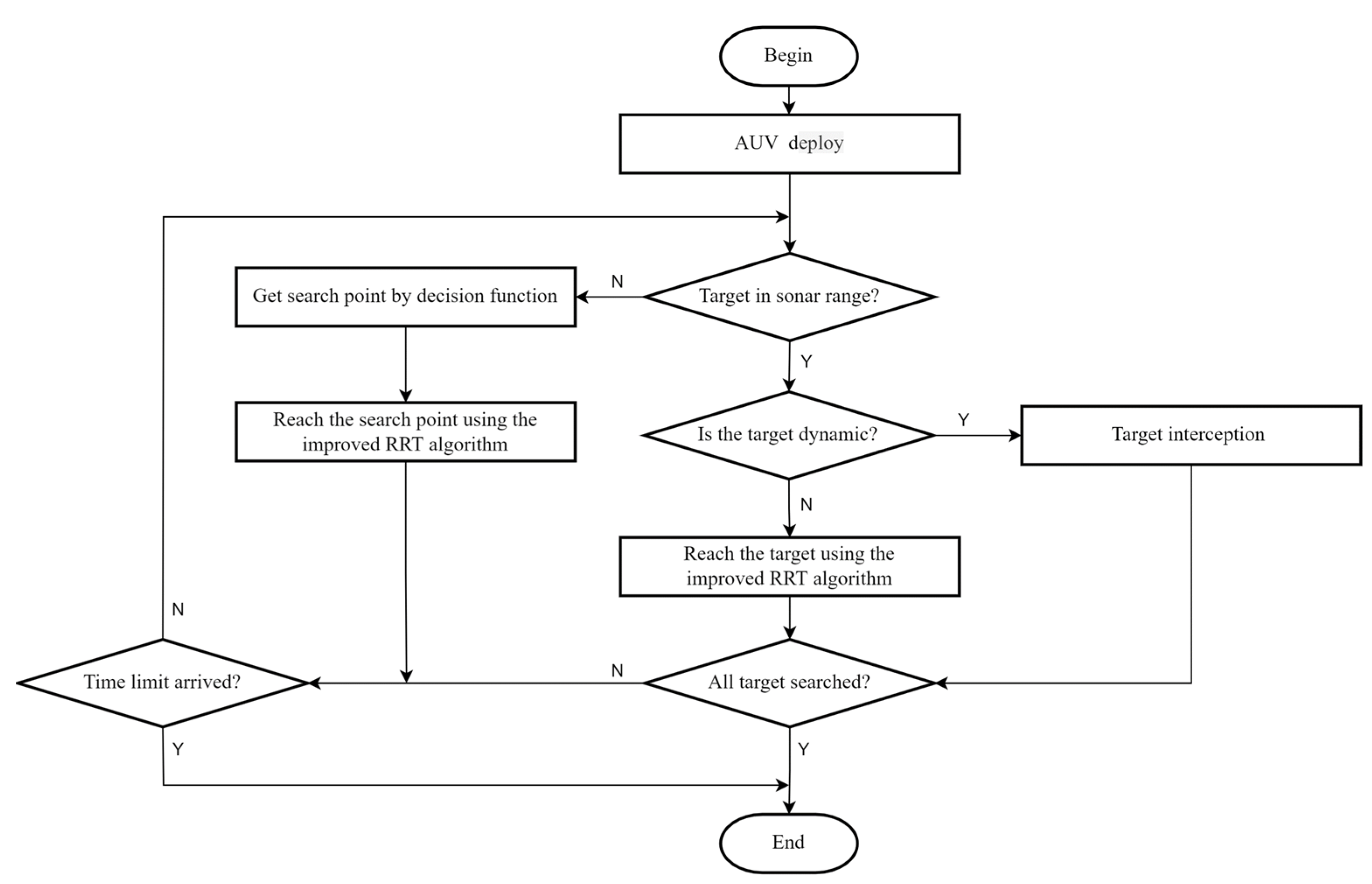
3. Three-Dimensional Environment Target Search Algorithm
3.1. Search Decision Function
- Improve the AUV’s awareness of environmental information;
- Avoid the rudder loss caused by frequent steering;
- Maximize the number of confirmed targets within a certain period of time.
3.1.1. Uncertainty Benefit
3.1.2. Search Task Benefit
3.1.3. Regional Ergodicity Benefit
3.2. Path Planning Based on the Improved RRT Algorithm
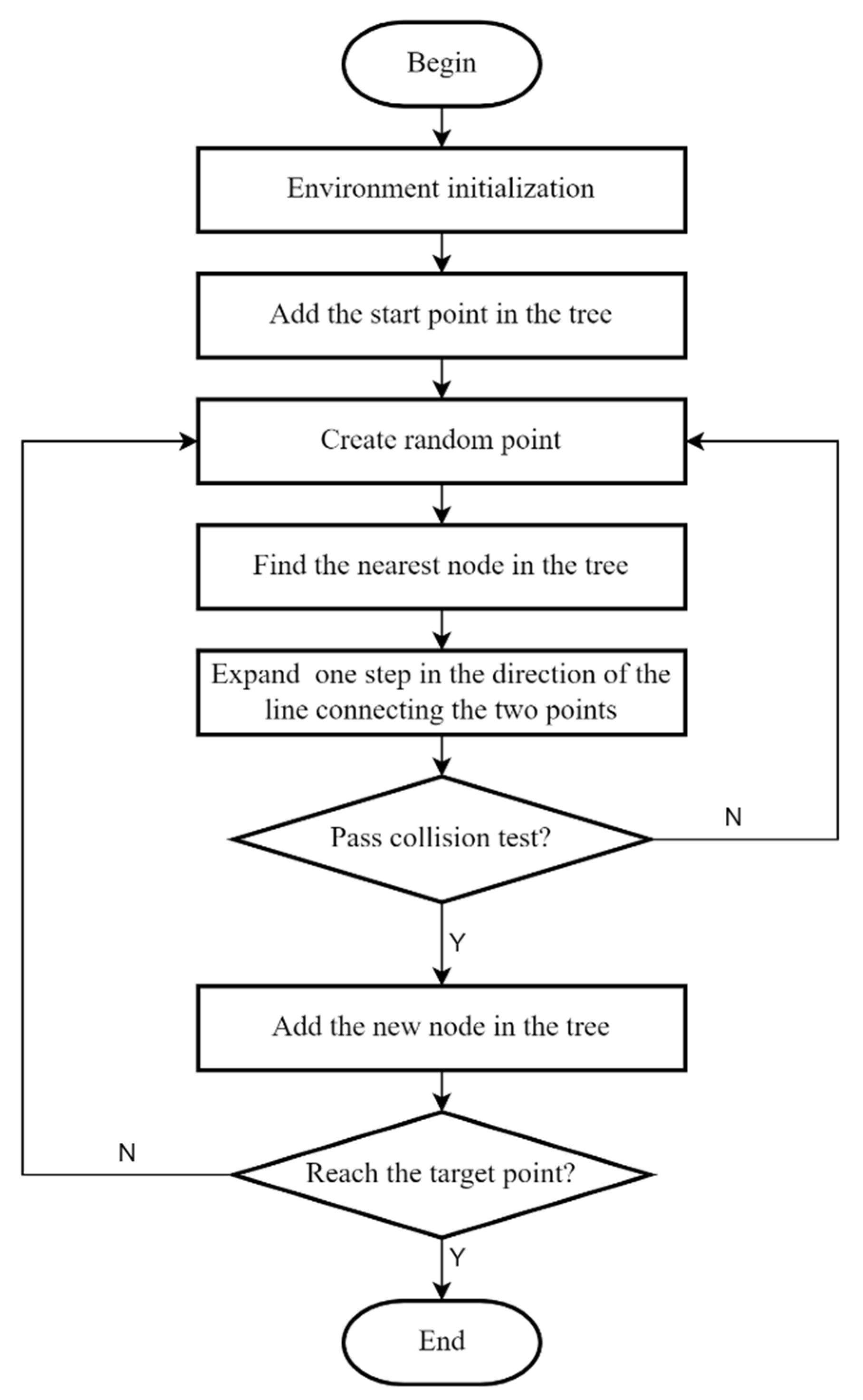
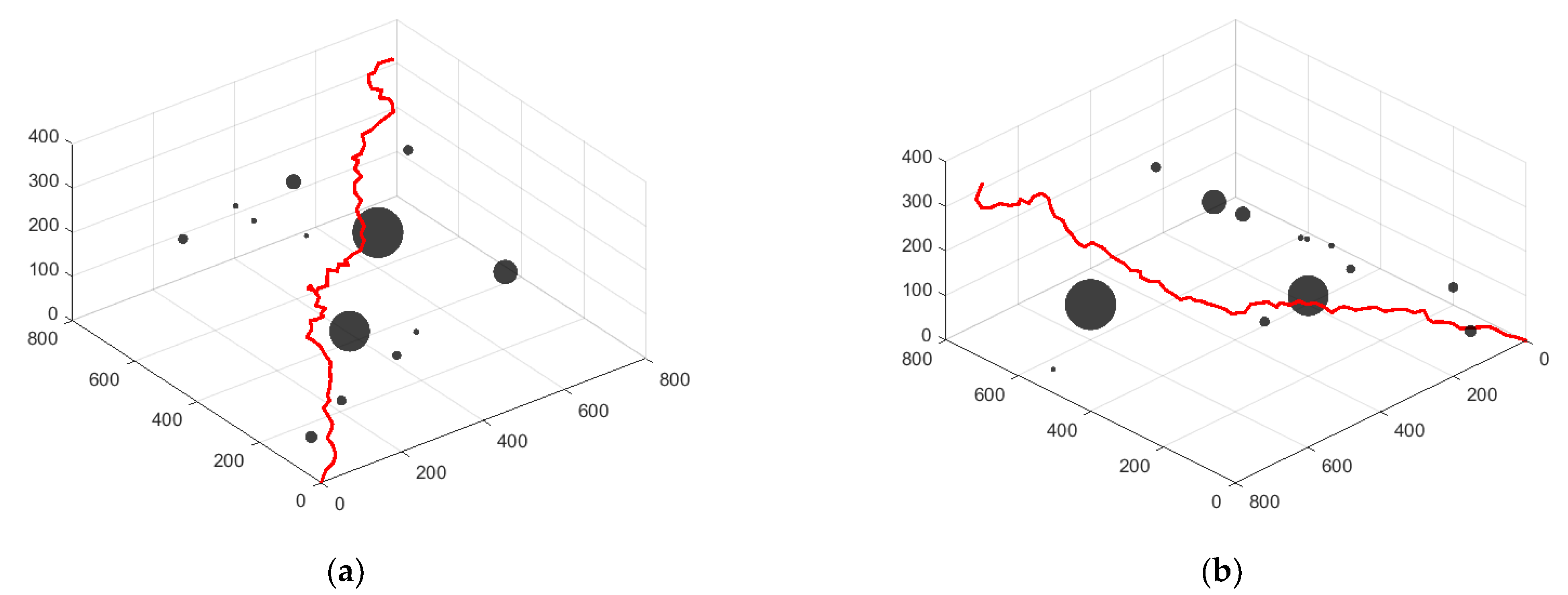
3.2.1. RRT Algorithm
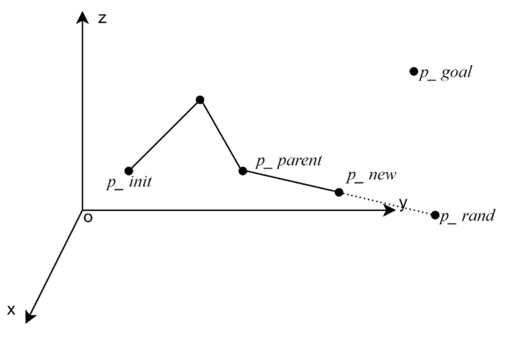
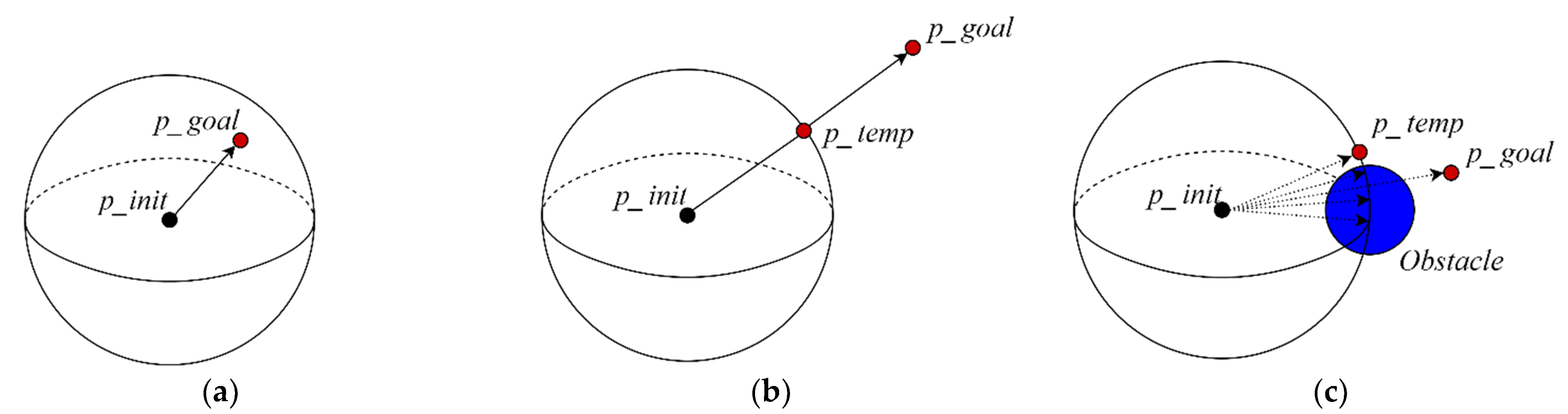
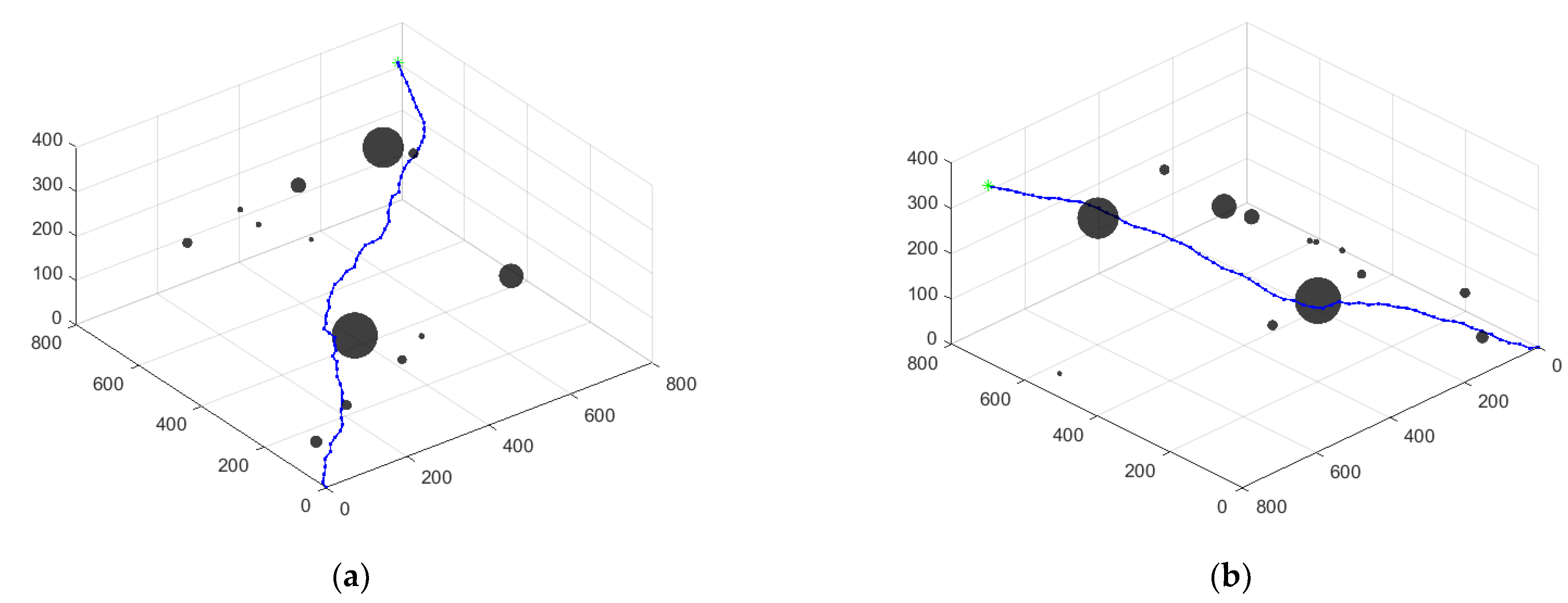
3.2.2. Improved RRT Algorithm
- 1.
- Rolling Planning
- 2.
- Sub-target Point Selection
- 3.
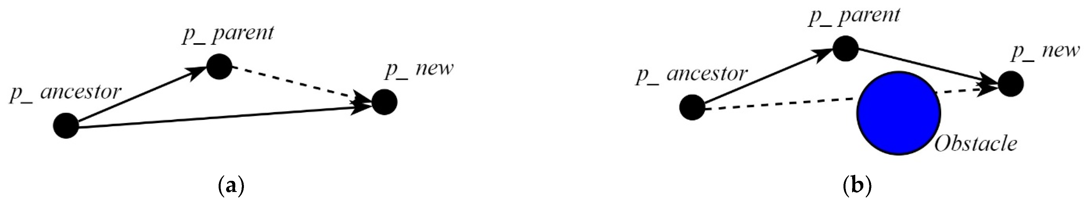
- Node Screening
- 4.
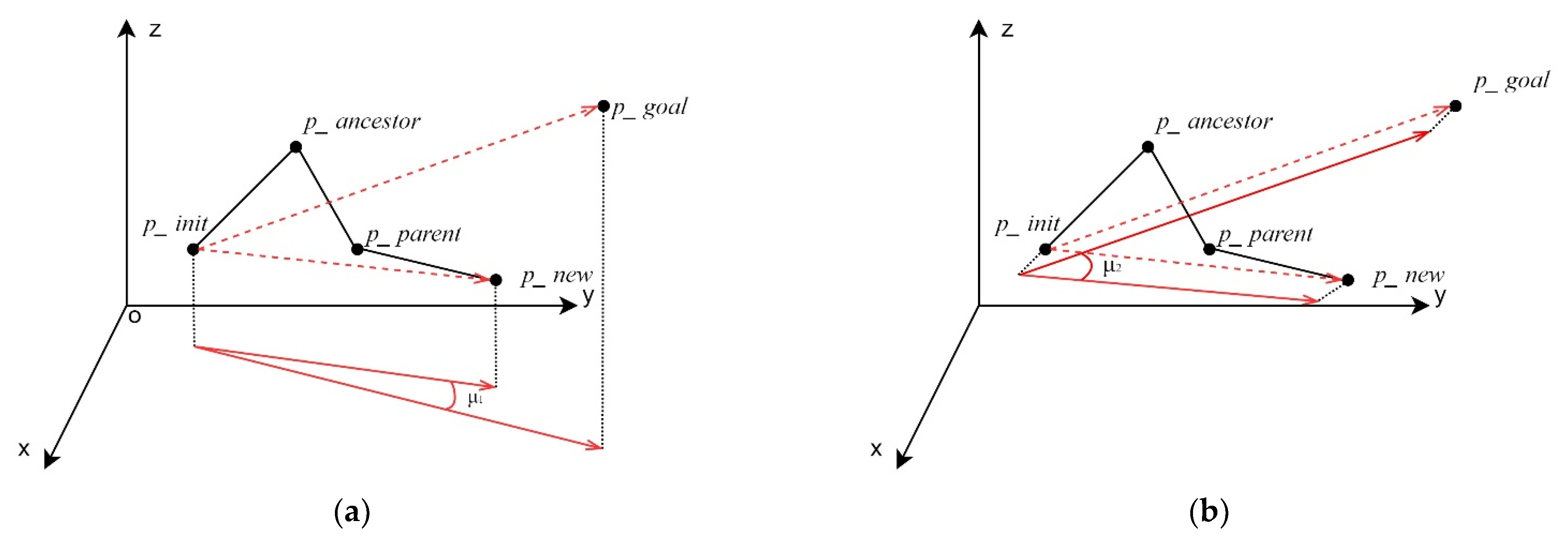
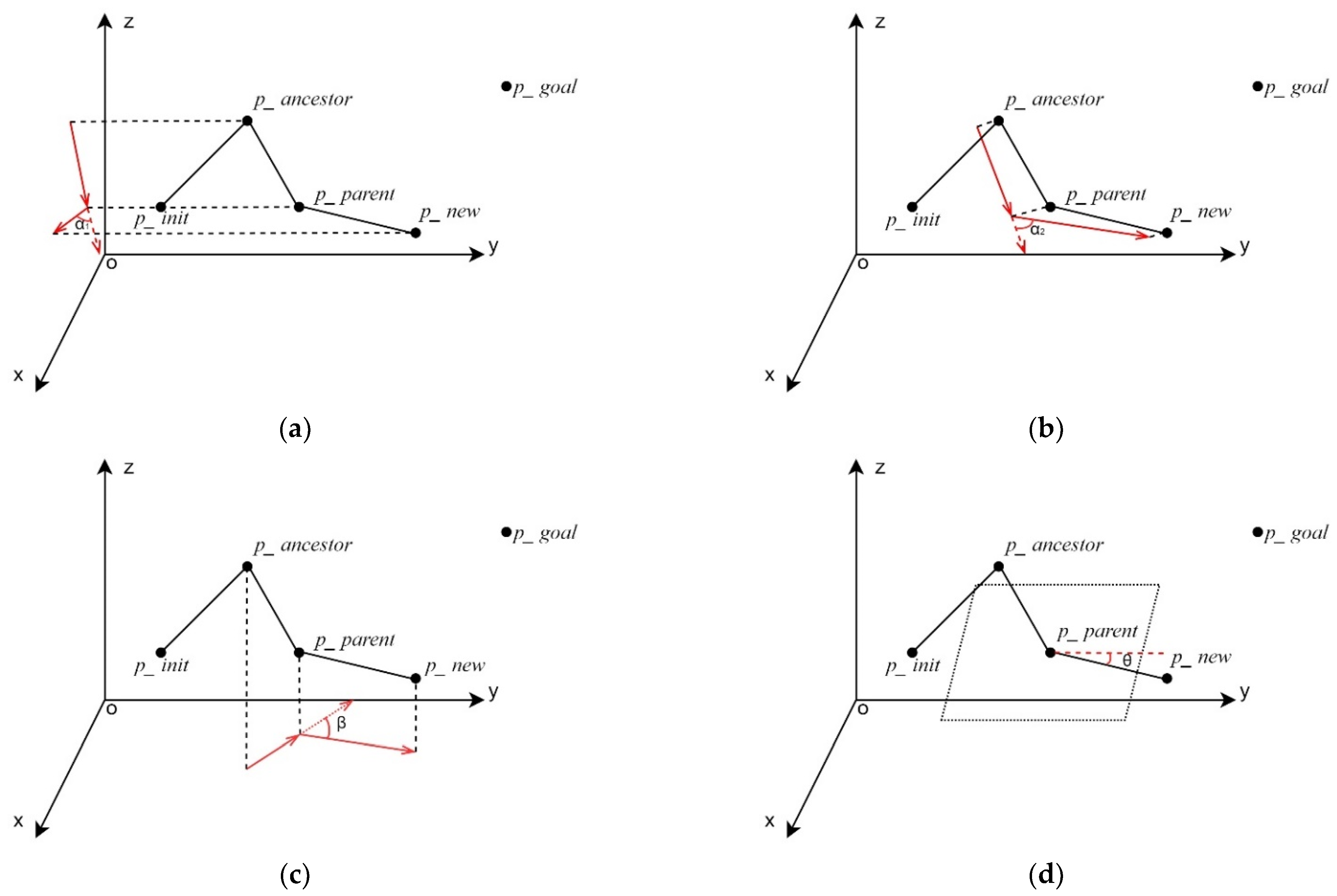
- Secondary Selection of the Parent Node
| Algorithm 1 Improved RRT Algorithm |
| pos = p_init |
| while ||p_new—p_goal|| ≤ d_min |
| V = { pos } |
| p_subtarget = Choose_subtarget(pos, p_goal) |
| for i = 1 to I do |
| p_rand = Random() |
| p_near = Nearest(V, p_rand) |
| p_new = Extend(p_near, r, p_rand) |
| if Collision_free(p_new, p_near) && Node_screen(p_new, p_near) then |
| Grow_tree(V, p_new) |
| Parent_node_selection (V, p_new) |
| end if |
| if ||p_new—p_subtarget || ≤ d_min then |
| pos = V(2) |
| break |
| end if |
| end for |
| end while |
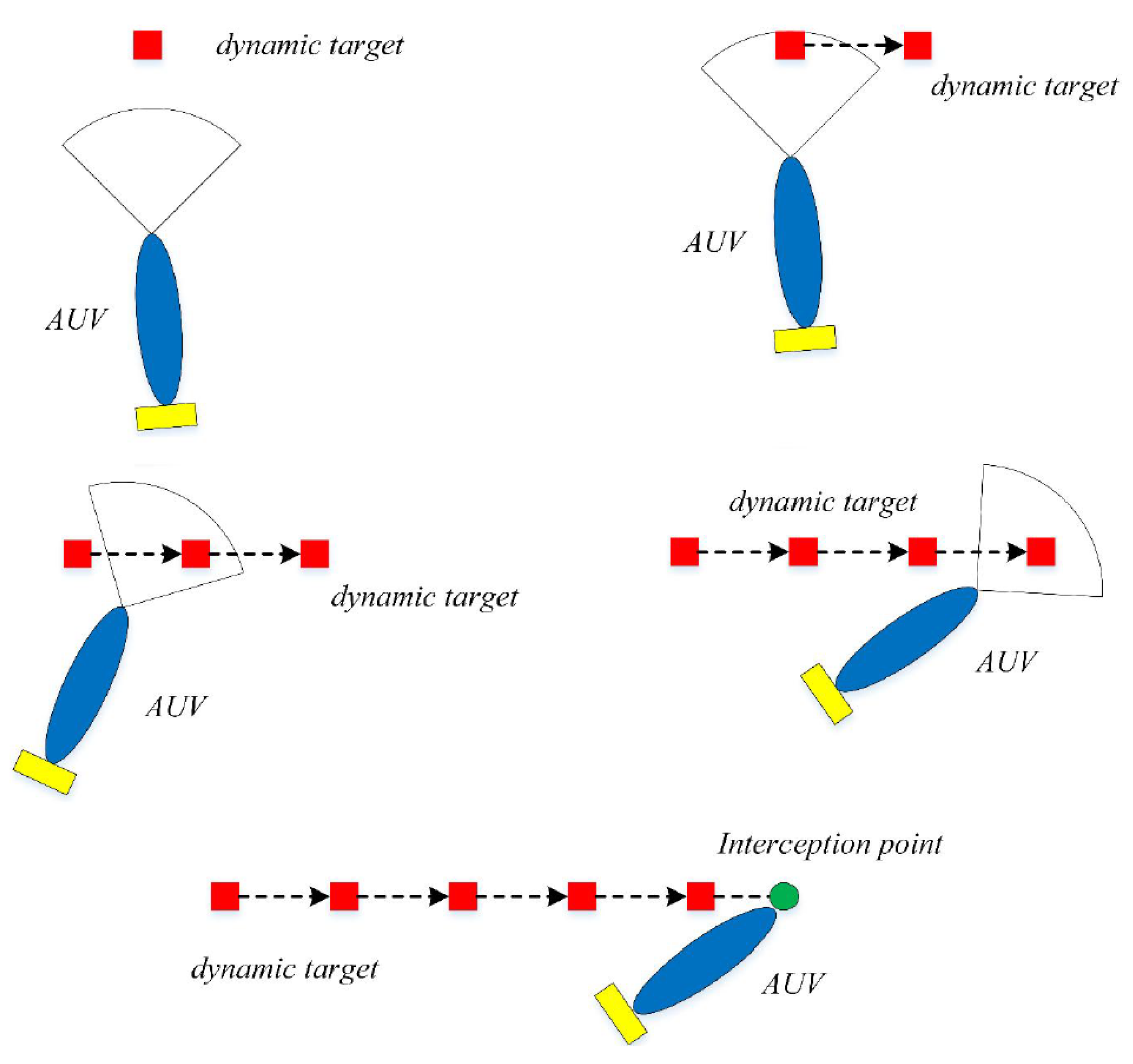
4. Target Interception Strategy
5. Simulation Results
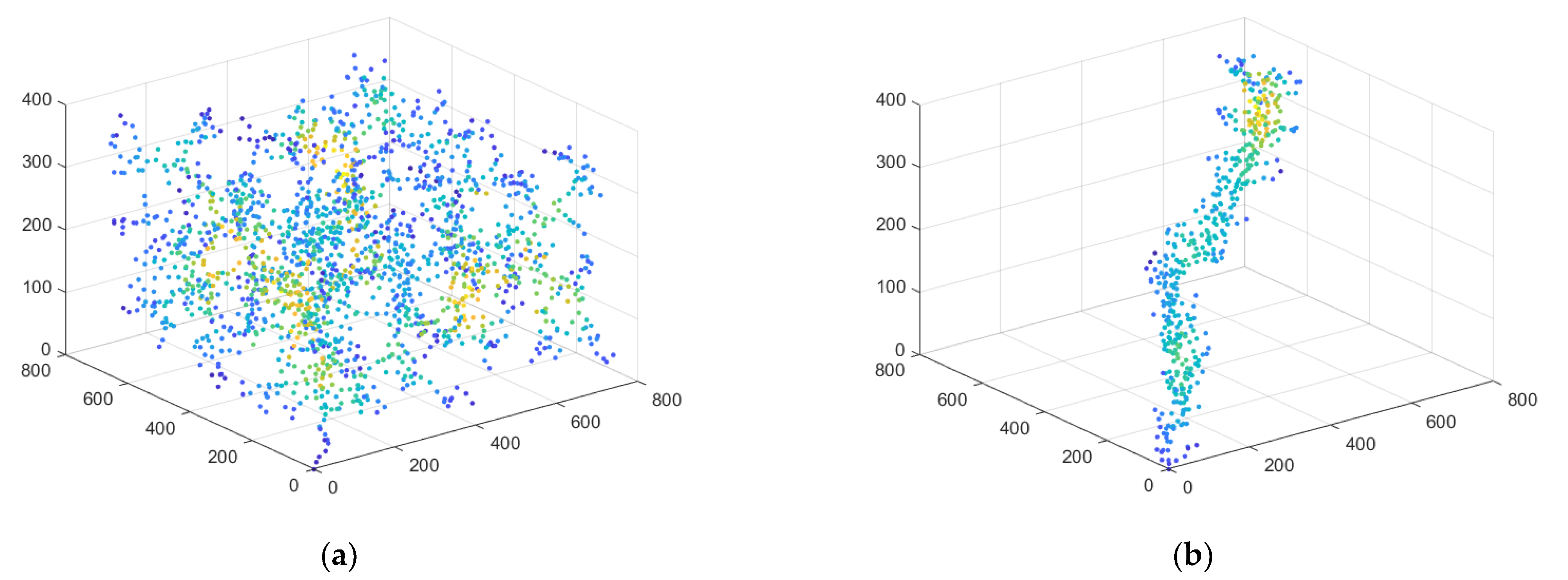
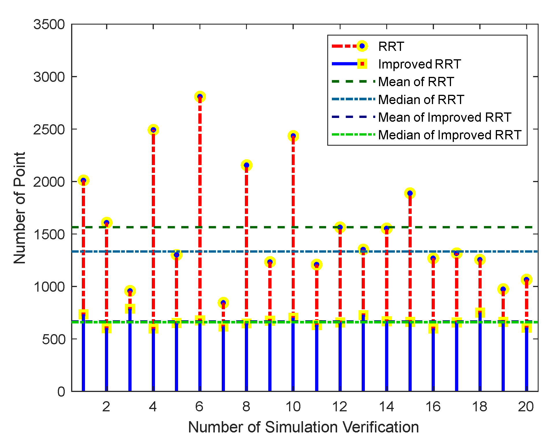
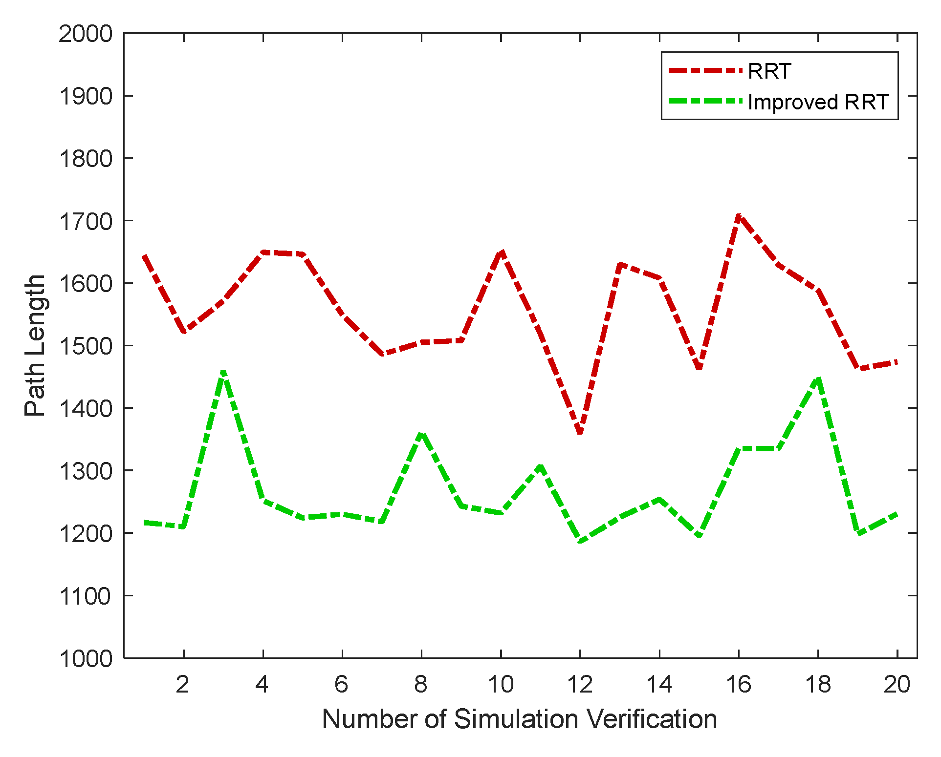
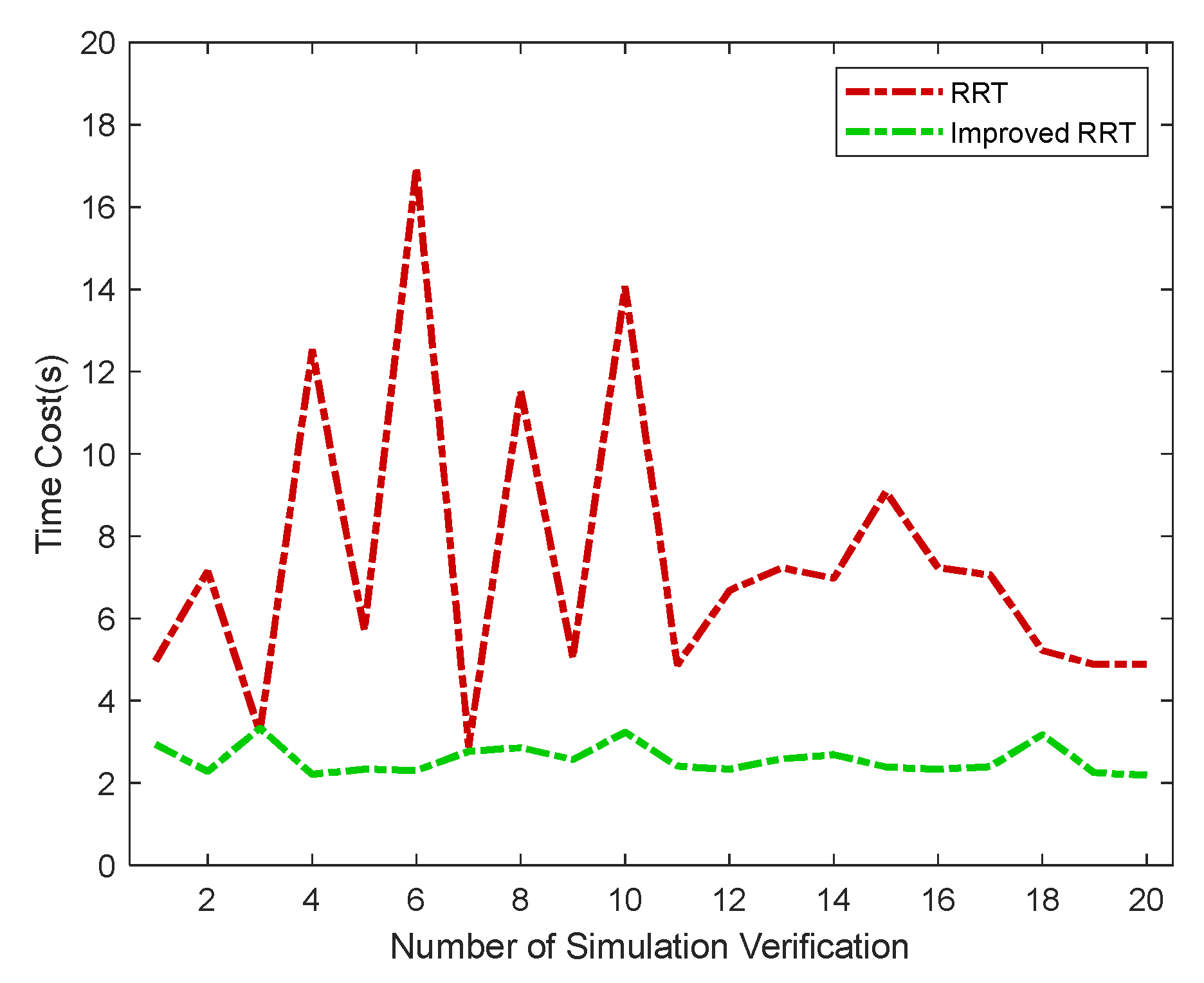
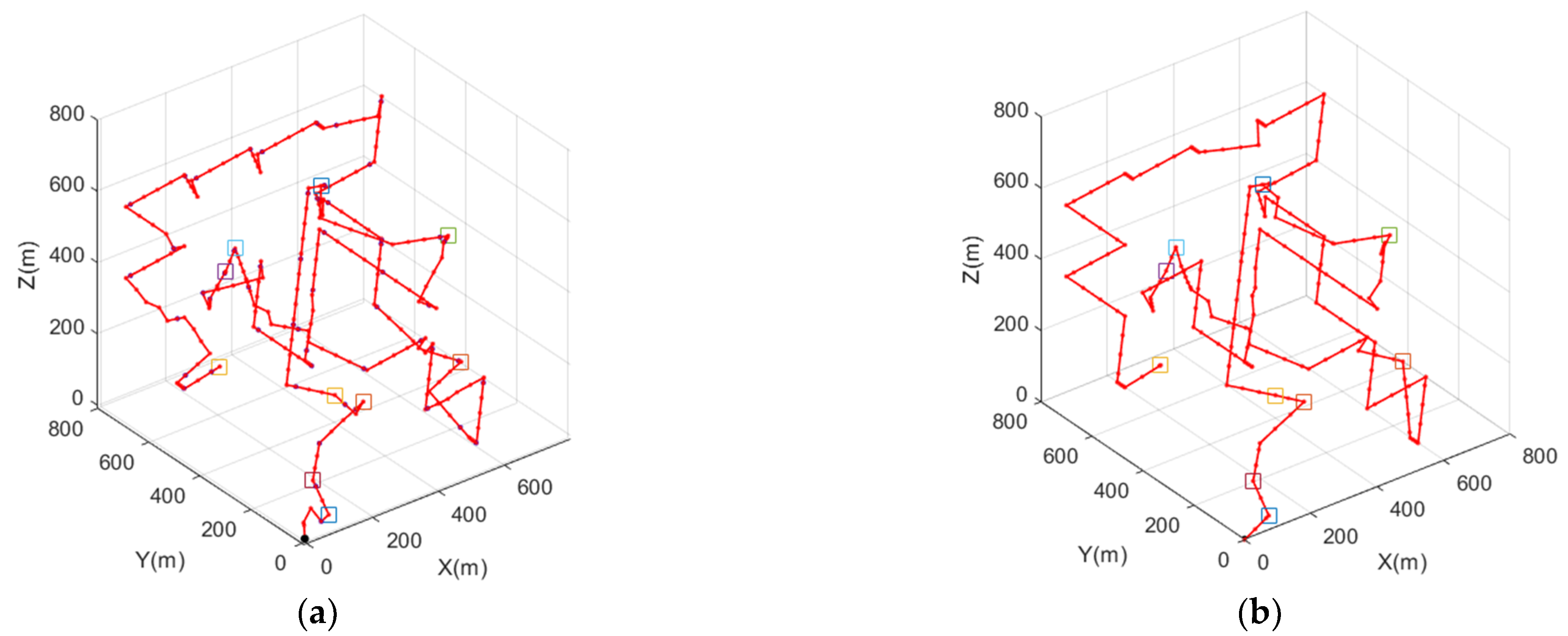
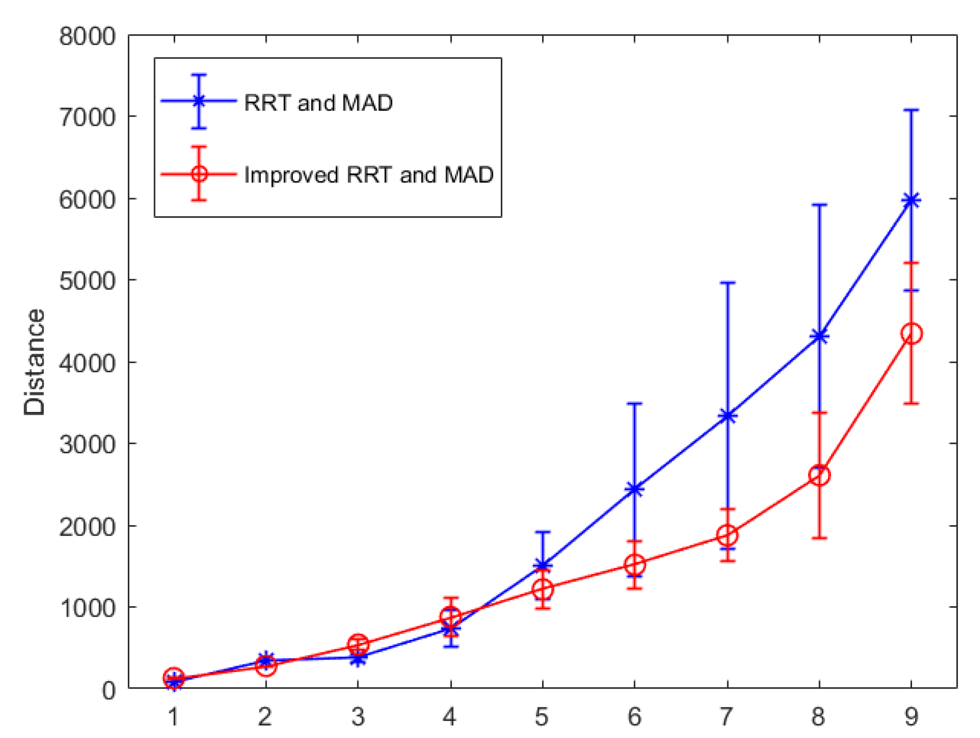
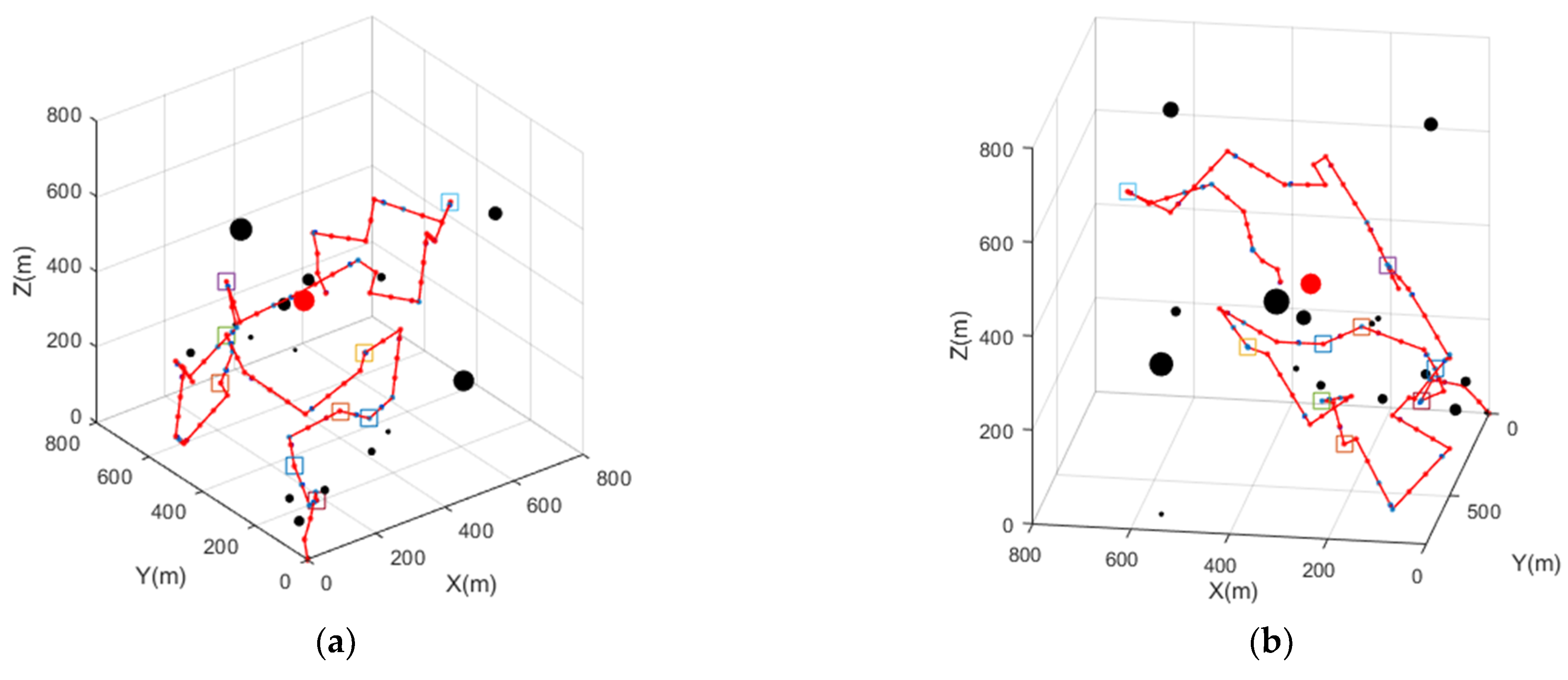
5.1. Improved RRT Algorithm Verification
5.2. Simulation of Target Search Algorithm in an Open Environment
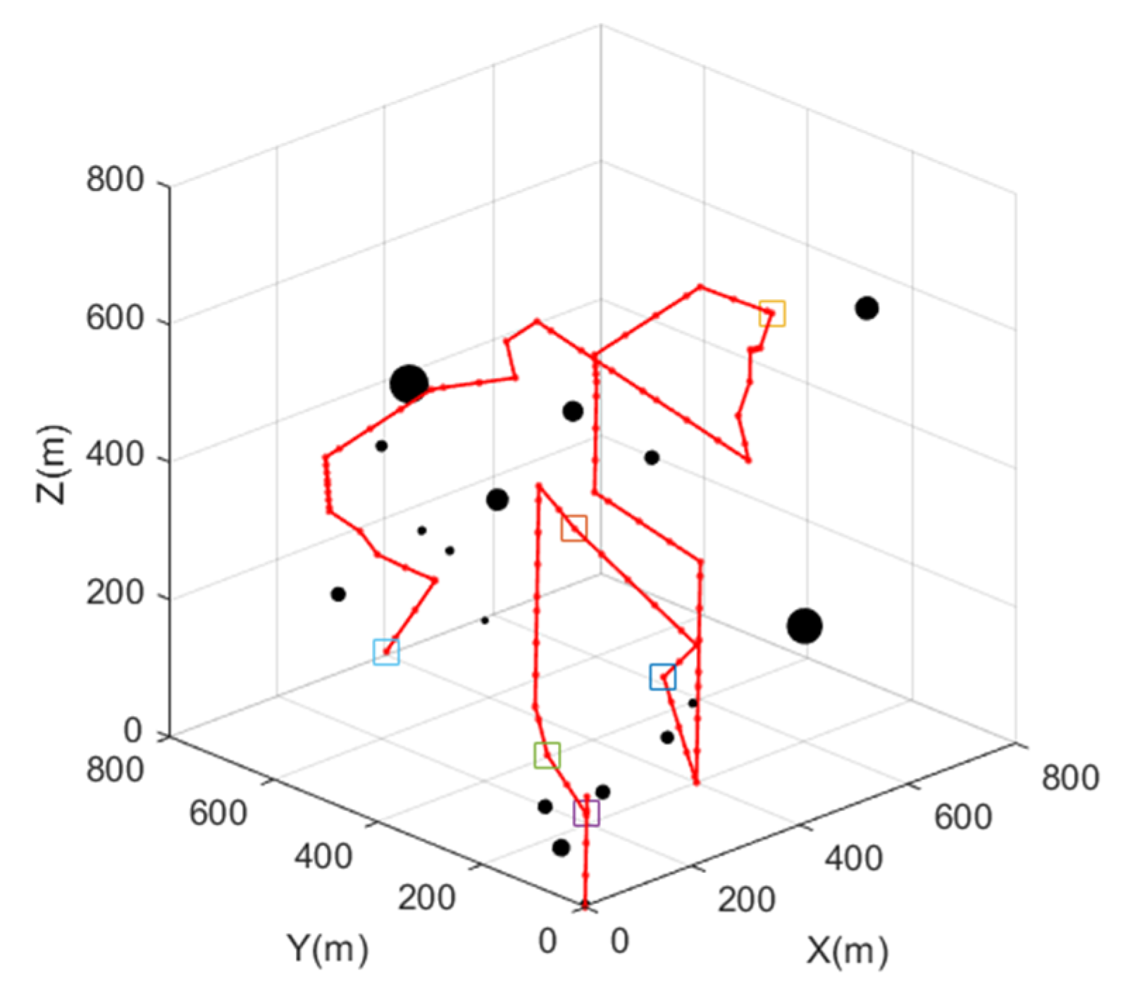
5.3. Simulation of Target Search Algorithm in an Obstacle Environment
5.4. Target Interception Algorithm Simulation
6. Conclusions
Author Contributions
Funding
Data Availability Statement
Conflicts of Interest
References
- Glaviano, F.; Esposito, R. Management and sustainable exploitation of marine environments through smart monitoring and automation. J. Mar. Sci. Eng. 2022, 10, 297. [Google Scholar] [CrossRef]
- Ru, J.; Yu, S.; Wu, H.; Li, Y.; Wu, C.; Jia, Z.; Xu, H. A multi-AUV path planning system based on the omni-directional sensing ability. J. Mar. Sci. Eng. 2021, 9, 806. [Google Scholar] [CrossRef]
- Liu, H.; Xu, B.; Liu, B. An automatic search and energy-saving continuous tracking algorithm for underwater targets based on prediction and neural network. J. Mar. Sci. Eng. 2022, 10, 283. [Google Scholar] [CrossRef]
- Chen, T.; Qu, X.; Zhang, Z.; Liang, X. Region-searching of multiple autonomous underwater vehicles: A distributed cooperative path-maneuvering control approach. J. Mar. Sci. Eng. 2021, 9, 355. [Google Scholar] [CrossRef]
- Mao, Y.; Gao, F.; Zhang, Q.; Yang, Z. An AUV Target-Tracking Method Combining Imitation Learning and Deep Reinforcement Learning. J. Mar. Sci. Eng. 2022, 10, 383. [Google Scholar] [CrossRef]
- Li, J.; Zhang, J. Target search of multiple autonomous underwater vehicles in an unknown environment. J. Harbin Eng. Univ. 2019, 40, 1951–1957, 1972. [Google Scholar]
- Ni, J.; Yang, L. An improved DSA-based approach for multi-AUV cooperative search. Comput. Intell. Neurosci. 2018, 2018, 2186574. [Google Scholar] [CrossRef] [PubMed]
- Ishida, T.; Korf, R.E. Moving-target search: A real-time search for changing goals. IEEE Trans. Pattern Anal. Mach. Intell. 1995, 15, 609–619. [Google Scholar] [CrossRef]
- Ajmera, Y.; Singh, S.P. Autonomous UAV-based target search, tracking and following using reinforcement learning and YOLOFlow. In Proceedings of the 2020 IEEE International Symposium on Safety, Security, and Rescue Robotics (SSRR), Abu Dhabi, United Arab Emirates, 4–6 November 2020. [Google Scholar]
- Wang, P.; Meghjani, M. Lost at sea: Multi-searcher multi-target search. In Proceedings of the Global Oceans 2020: Singapore—U.S. Gulf Coast, Biloxi, MS, USA, 5–30 October 2020. [Google Scholar]
- Ibenthal, J.; Meyer, L.; Piet-Lahanier, H. Target search and tracking using a fleet of UAVs in presence of decoys and obstacles. In Proceedings of the 59th IEEE Conference on Decision and Control (CDC), Jeju, Korea, 14–18 December 2020. [Google Scholar]
- Yin, G.; Zhou, S.; Wu, Q. An improved RRT algorithm for UAV path planning. Acta Electron. Sin. 2017, 45, 1764. [Google Scholar]
- Wu, X.G.; Guo, C.; Li, Y.B. Variable probability based bidirectional RRT algorithm for UAV path planning. In Proceedings of the 26th Chinese Control and Decision Conference (2014 CCDC), Changsha, China, 31 May–2 June 2014. [Google Scholar]
- Guo, Y.; Liu, X.; Liu, X.; Yang, Y.; Zhang, W. FC-RRT*: An improved path planning algorithm for UAV in 3D complex environment. ISPRS Int. J. Geo-Inf. 2022, 11, 112. [Google Scholar] [CrossRef]
- Li, J.; Zhang, Y.X. Formation control of a multi-autonomous underwater vehicle event-triggered mechanism based on the hungarian algorithm. Machines 2022, 9, 346. [Google Scholar] [CrossRef]
- Li, J.; Zhai, X.L. Target search algorithm for AUV based on real-time perception maps in unknown environment. Machines 2021, 9, 147. [Google Scholar] [CrossRef]
- Hu, J.W.; Xie, L.; Xu, J.; Xu, Z. Multi-Agent Cooperative Target Search. Sensors 2014, 14, 9408–9428. [Google Scholar] [CrossRef] [PubMed] [Green Version]
- Song, D.L.; Yao, P. Search for static target in nonwide area by AUV: A prior data-driven strategy. IEEE Syst. J. 2021, 15, 3185–3188. [Google Scholar] [CrossRef]
- Zhu, J.; Zhao, S.; Zhao, R. Path planning for autonomous underwater vehicle based on artificial potential field and modified RRT. In Proceedings of the 2021 International Conference on Computer, Control and Robotics (ICCCR), Shanghai, China, 8–10 January 2021. [Google Scholar]
- Cho, Y.; Kim, E. Path planning of a robot manipulator using retrieval RRT strategy. Int. J. Fuzzy Logic Intell. Syst. 2007, 7, 138–142. [Google Scholar]
- Wang, R.P.; Xi, W.; Guo, X. Path following for snake robot using crawler gait based on path integral reinforcement learning. In Proceedings of the 6th IEEE International Conference on Advanced Robotics and Mechatronics (ICARM), Chongqing, China, 3–5 July 2021. [Google Scholar]
- Guo, H.; Qin, J.L. Rolling path planning of mobile robot based on automatic diffluence ant algorithm. In Proceedings of the 12th International Conference on Graphics and Image Processing (ICGIP), Xi’an, China, 13–15 November 2020. [Google Scholar]
- Kang, J.G.; Lim, D.W. Improved RRT-connect algorithm based on triangular inequality for robot path planning. Sensors 2021, 21, 333. [Google Scholar] [CrossRef] [PubMed]
- Meng, X.Q.; Sun, B. Harbour protection: Moving invasion target interception for multi-AUV based on prediction planning interception method. Ocean Eng. 2021, 219, 108268. [Google Scholar] [CrossRef]


| Algorithm | Optimization Methods | Merit | Deficiency |
|---|---|---|---|
| RNR-RRT | The selection strategy of the root node is improved. | B-spline curve trace smoothing Turn angle constraint Track distance constraint | 2D environment |
| VPB-RRT | The offset of the new node is determined by the map coverage. | Rasterizing the planning space Import coverage rate Turn angle constraint | Tendency to create a local optimal solution |
| FC-RRT* | The flight cost function is used to inspire the expansion of new nodes and guide the update of the parent node. | Complex 3D environment Flight constraints Improved path safety | Excessive number of nodes |
| Number of Nodes | Path Length | Time Cost | Number of Nodes | Path Length | Time Cost |
|---|---|---|---|---|---|
| 1209 | 1644 | 4.97 | 1209 | 1518 | 4.87 |
| 1609 | 1522 | 7.15 | 1564 | 1359 | 6.68 |
| 958 | 1571 | 3.22 | 1353 | 1630 | 7.23 |
| 2492 | 1649 | 12.54 | 1553 | 1608 | 6.98 |
| 1301 | 1646 | 5.71 | 1888 | 1462 | 9.08 |
| 2809 | 1549 | 16.94 | 1268 | 1709 | 7.23 |
| 844 | 1486 | 2.87 | 1315 | 1629 | 7.06 |
| 2155 | 1505 | 11.53 | 1256 | 1588 | 5.22 |
| 1234 | 1508 | 5.03 | 974 | 1462 | 4.88 |
| 2434 | 1653 | 14.08 | 1065 | 1474 | 4.89 |
| Number of Nodes | Path Length | Time Cost | Number of Nodes | Path Length | Time Cost |
|---|---|---|---|---|---|
| 735 | 1217 | 2.94 | 633 | 1307 | 2.41 |
| 602 | 1210 | 2.28 | 658 | 1186 | 2.34 |
| 802 | 1459 | 3.34 | 728 | 1225 | 2.59 |
| 598 | 1252 | 2.21 | 669 | 1254 | 2.69 |
| 652 | 1224 | 2.34 | 663 | 1195 | 2.39 |
| 677 | 1230 | 2.31 | 599 | 1335 | 2.33 |
| 619 | 1218 | 2.77 | 657 | 1335 | 2.40 |
| 648 | 1362 | 2.86 | 752 | 1450 | 3.18 |
| 675 | 1243 | 2.57 | 662 | 1198 | 2.25 |
| 701 | 1232 | 3.24 | 608 | 1231 | 2.19 |
| Target Code | X/m | Y/m | Z/m |
|---|---|---|---|
| 1 | 104 | 40 | 10 |
| 2 | 310 | 170 | 190 |
| 3 | 230 | 178 | 234 |
| 4 | 130 | 477 | 476 |
| 5 | 630 | 250 | 500 |
| 6 | 200 | 530 | 490 |
| 7 | 118 | 120 | 63 |
| 8 | 430 | 490 | 600 |
| 9 | 600 | 160 | 200 |
| 10 | 200 | 590 | 130 |
| Algorithm | Time/s | Path Length/m |
|---|---|---|
| Conventional RRT | 30,681 | 61,367 |
| Improved RRT | 21,987 | 43,969 |
| Target Code | X/m | Y/m | Z/m |
|---|---|---|---|
| 1 | 310 | 170 | 190 |
| 2 | 350 | 383 | 328 |
| 3 | 680 | 345 | 555 |
| 4 | 118 | 120 | 63 |
| 5 | 84 | 160 | 147 |
| 6 | 200 | 590 | 130 |
| Target Code | X/m | Y/m | Z/m |
|---|---|---|---|
| 1 | 30 | 108 | 104 |
| 2 | 315 | 168 | 101 |
| 3 | 545 | 758 | 20 |
| 4 | 168 | 435 | 334 |
| 5 | 52 | 100 | 40 |
| 6 | 115 | 85 | 107 |
| 7 | 150 | 470 | 358 |
| 8 | 365 | 171 | 135 |
| 9 | 300 | 480 | 355 |
| 10 | 564 | 456 | 345 |
| 11 | 324 | 675 | 456 |
| 12 | 98 | 125 | 654 |
| 13 | 630 | 230 | 150 |
| 14 | 630 | 110 | 650 |
| 15 | 120 | 600 | 234 |
| 16 | 210 | 610 | 420 |
| Target Code | X/m | Y/m | Z/m |
|---|---|---|---|
| 1 | 310 | 170 | 190 |
| 2 | 230 | 178 | 234 |
| 3 | 434 | 349 | 238 |
| 4 | 130 | 477 | 476 |
| 5 | 240 | 620 | 230 |
| 6 | 680 | 345 | 555 |
| 7 | 118 | 120 | 63 |
| 8 | 84 | 160 | 147 |
| 9 | 200 | 590 | 130 |
Publisher’s Note: MDPI stays neutral with regard to jurisdictional claims in published maps and institutional affiliations. |
© 2022 by the authors. Licensee MDPI, Basel, Switzerland. This article is an open access article distributed under the terms and conditions of the Creative Commons Attribution (CC BY) license (https://creativecommons.org/licenses/by/4.0/).
Share and Cite
Li, J.; Li, C.; Chen, T.; Zhang, Y. Improved RRT Algorithm for AUV Target Search in Unknown 3D Environment. J. Mar. Sci. Eng. 2022, 10, 826. https://doi.org/10.3390/jmse10060826
Li J, Li C, Chen T, Zhang Y. Improved RRT Algorithm for AUV Target Search in Unknown 3D Environment. Journal of Marine Science and Engineering. 2022; 10(6):826. https://doi.org/10.3390/jmse10060826
Chicago/Turabian StyleLi, Juan, Chengyue Li, Tao Chen, and Yun Zhang. 2022. "Improved RRT Algorithm for AUV Target Search in Unknown 3D Environment" Journal of Marine Science and Engineering 10, no. 6: 826. https://doi.org/10.3390/jmse10060826