Comparison of the Hydraulic Performance and Pressure Pulsation Characteristics of Shaft Tubular Pump Device under Multiple Working Conditions

Abstract

For pumping station projects in plain areas, shaft tubular pump devices are often used due to the low head. In actual operation, the common working range of the pump device is generally 0.8 Q_bep~1.2 Q_bep. Therefore, it is of great significance to study the hydraulic performance and pressure pulsation characteristics of the pump device in the working range. In this study, the hydraulic performance of a shaft pump device was tested by a model test, and the internal flow and pressure pulsation characteristics were analyzed by numerical simulation. The results obtained from the model test and numerical simulation were in general agreement, indicating that the numerical results were reliable. The results show that the inlet passage has a good flow pattern in the working range, which may offer a favorable flow state for the impeller. When Q = 0.8 Q_bep, the flow in the impeller and guide vane was chaotic, the guide vane had a poor adjustment function on flow direction, and the flow in the outlet passage presented in a spiral motion. When Q = 1.0 and 1.2 Q_bep, the flow in the impeller and guide vane was ordered, and the spiral flow in the outlet passage improved. In the working range, the pressure pulsation was similar. The main frequency at the impeller inlet and outlet was consistent with the blade passing frequency. For the same flow rate condition, the amplitude rose from hub to shroud and declined from impeller inlet to outlet. In addition, the amplitude decreased with an increasing flow rate.

1. Introduction

Pumping stations are an indispensable part of the water conservancy project, which plays an important role in urban drainage, flood control, and inter-basin water transfer [1,2]. The shaft tubular pump device is frequently utilized in practical applications due to its benefits of outstanding hydraulic performance and simple structure [3,4]. A great deal of research has already been conducted on the shaft tubular pump device. Xu et al. [5] compared the performance of different schemes of shaft tubular pump devices and verified it by a test. The highest efficiency was over 83%, which shows the pump device is suitable for promotion. Lu et al. [6] studied the hydraulic performance under different blade mounting angles by a test, and the result showed that the highest efficiency was 78.83%. Jiao et al. [7] studied the effect of inlet guide vanes on the hydraulic performance of shaft tubular pumps, and the results show that the number of inlet guide vanes has a considerable impact on the performance. As the number of IGVs increases, the impeller inlet pressure pulsation amplitude first decreases and then increases under the small and design flow rate conditions; however, it gradually increases under large flow rate conditions. Zhou et al. [8] also studied the influence of shaft profile on hydraulic performance; the study found that the inlet passage with a cone-shaped head profile and tail profile had better hydraulic performance. Xu et al. [9] conducted a study on the design parameters of the outlet passage of the shaft tubular pump device and proposed that the plane diffusion angle should be about 17°, and the façade diffusion angle should be less than 7°.

In the operation of the pump, pressure pulsation is a common phenomenon, which leads to vibration damage of the unit in severe cases [10,11,12,13]. Gonzalez et al. [14] used a centrifugal pump as the sample of the study. The study revealed that pump vibration is directly related to unsteady pressure pulsation. Arndt et al. [15,16] conducted an experimental study of pressure pulsation in a centrifugal pump and found that the pressure pulsation is circumferential inhomogeneity, and the pulsation amplitude at the impeller outlet is the largest. Al-Obaidi [17] studied pressure pulsation under different blade angles by CFD. It was found that the blade angles had great influence on the amplitude of fluctuation. Zhang et al. [18] investigated pressure pulsation under design conditions at various rotational speeds and proposed that when rotational speed decreased, the major frequency moved to the high-frequency zone. Li et al. [19] found that the main frequency of the axial-flow pump is the blade passing frequency.

In the past, the studies on the shaft tubular pump device mainly focused on the hydraulic performance and pressure pulsation under optimal working conditions, as well as the optimization design of the inlet and outlet passages. However, in actual operation, the common working range of the shaft tubular pump device is generally 0.8 Q_bep~1.2 Q_bep. Therefore, it is of great significance to study the hydraulic performance and pressure pulsation characteristics of the shaft tubular pump device in the working range. However, there have been few studies on the hydraulic performance and pressure pulsation of the shaft tubular pump device under different operating conditions in the working range. In order to supplement the previous studies, this paper systematically investigated the hydraulic performance and pressure pulsation characteristics in the working range of the shaft tubular pump device by numerical simulation, and the accuracy of the numerical simulation was verified by a model test. This paper clearly shows the hydraulic performance and pressure pulsation characteristics of the shaft tubular pump device in the working range and can provide better guidance for the stable and efficient operation of the shaft tubular pump device.

2. CFD Method

2.1. Simulation Model and Settings

Different from the traditional definition of an axial-flow pump, the axial-flow pump device is composed of an inlet passage, an axial-flow pump, and an outlet passage. This study took a large-scaled pumping station as the research object, which was equipped with a shaft tubular pump device. UG software was used to model the inlet and outlet passage. Turbo-Grid software was used to model the pump. The pump had 3 blades and 5 guide vanes, the impeller diameter was 0.3 m, and the tip clearance of the impeller was set as 0.15 mm. The software used in this numerical simulation was CFX, and the post-processing software was CFD-POST and Tecplot. The simulation model is visualized in Figure 1.

Table 1. Numerical simulation settings.

Parameter	Settings
Inlet of the model	Total pressure (1 atm)
Outlet of the model	Mass flow rate
Wall of the model	No-slip
Time step	1.15 × 10−4 s (1 degree impeller rotation time)
Total time	0.331 s (8 cycles impeller rotation time)
Dynamic and static interface (Steady Simulation)	Stage
Dynamic and static interface (Unsteady Simulation)	Transient rotor and stator
Static and static interface	None
Convergence accuracy	1 × 10−4

shows the basic settings of the numerical simulation.

2.2. Turbulence Model

In the past, the research on rotating machinery mainly relied on experiments and theoretical analysis. However, the model test has the disadvantages of taking a long period of time, complex operation, and high costs. CFD has been widely used in the study of the axial-flow pump [20,21,22,23], centrifugal pump [24,25,26,27], and pump as turbine [28]. The time-averaged Navier–Stokes equation was used to describe the flow in this numerical simulation [29,30]. The “RNG k-ε” model was adopted in this research because of its benefit in addressing the flow field of rotating machinery [31,32,33]. The equations are as follows.

$$\frac{\partial \left(\rho k\right)}{\partial t}+\frac{\partial \left(\rho k{u}_i\right)}{\partial x_i}=\frac{\partial }{\partial x_j}\left[{\alpha }_k{\mu }_{eff}\frac{\partial k}{\partial x_j}\right]+{\mu }_t\left(\frac{\partial u_i}{\partial x_j}+\frac{\partial u_j}{\partial x_i}\right)\frac{\partial u_i}{\partial x_j}-\rho \epsilon ,$$

(1)

$$\frac{\partial \left(\rho \epsilon \right)}{\partial t}+\frac{\partial \left(\rho \epsilon u_i\right)}{\partial x_i}=\frac{\partial }{\partial x_j}\left[{\alpha }_{\epsilon }{\mu }_{eff}\frac{\partial \epsilon }{\partial x_j}\right]+\frac{C_{\epsilon 1}}{k}{\mu }_t\left(\frac{\partial u_i}{\partial x_j}+\frac{\partial u_j}{\partial x_i}\right)\frac{\partial u_i}{\partial x_j}-C_{\epsilon 2}\rho \frac{{\epsilon }^2}{k}-R,$$

(2)

where ${\mu }_{eff}$ is the effective viscosity of turbulence. k is the turbulence energy. $\epsilon$ is the dissipation rate of the turbulent kinetic energy. ${\mu }_{eff}=\mu +{\mu }_t$. $R=\frac{C_{\mu }\rho {\eta }^3\left(1-\eta /{\eta }_0\right)}{1+\beta {\eta }^3}·\frac{{\epsilon }^2}{k}$. $\eta ={\left(2E_{ij}·E_{ij}\right)}^{1/2}\frac{k}{\epsilon }$. $E_{ij}=\frac{1}{2}\left(\frac{\partial u_i}{\partial x_j}+\frac{\partial u_j}{\partial x_i}\right)$. ${\eta }_0$ = 4.377. $\beta$ = 0.012. ${\sigma }_k$ = ${\sigma }_{\epsilon }$ = 1.39.

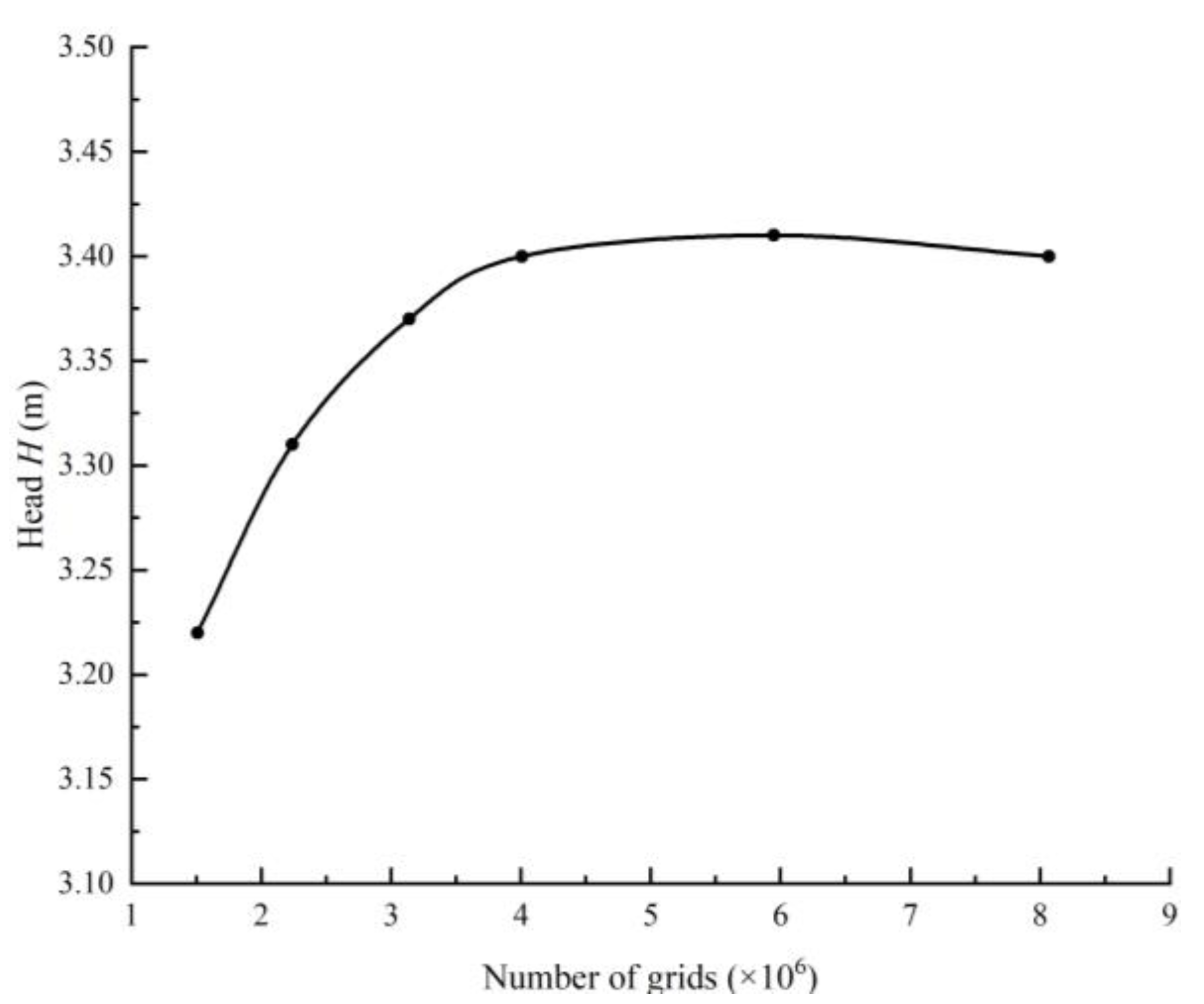
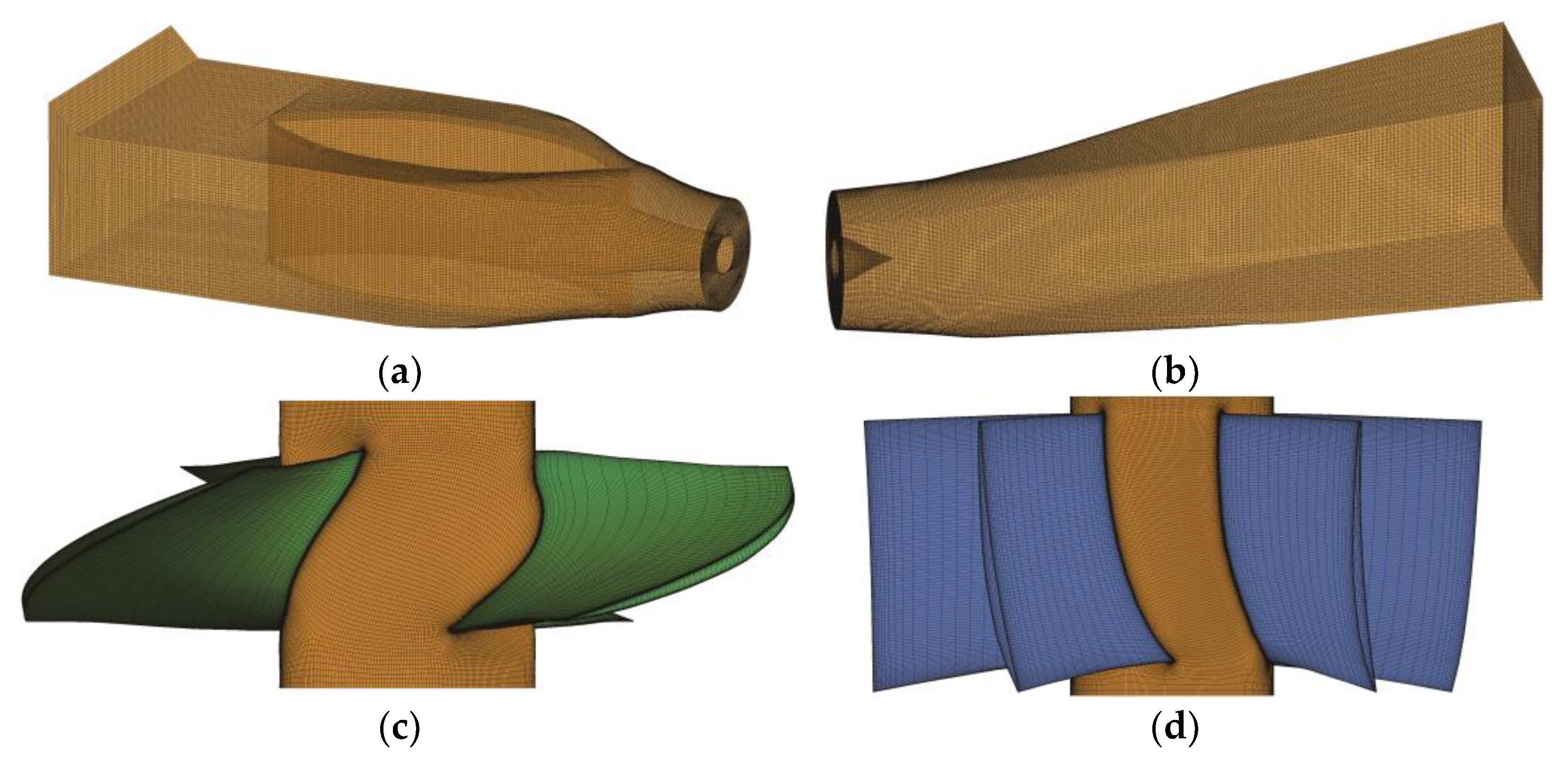
2.3. Calculation Grid and Independence Verification

The grid is divided into structured and unstructured grids. In this study, the flow passages were divided into structured grids via ICEM, and the impeller and guide vane were divided into structured grids via Turbo-Grid. The boundary layer grid was encrypted at the wall surface.

From the theoretical perspective, the more the number of grids in the model, the more accurate the calculation result will be. However, the relationship between the result and the number of grids is not linear; once the amount of grids exceeds a particular number, the outcome is almost unaffected. Six sets of grid schemes were divided in this study, and the skewness was less than 0.8. The heads of different schemes are shown in Figure 2.

As shown in Figure 2, it was found that once the amount of grids reached 4.01 million, the heads changed very minimally, the absolute value of change was less than 0.01 m, and the relative change value was less than 0.3%, meeting the requirements of grid independence. Furthermore, the grid convergence index (GCI) was used to verify the grid reliability. The convergence error ∋, average grid spacing h, grid encryption ratio r, and GCI can be calculated by the following formulas:

$$\ni =\frac{f_i-f_{i+1}}{f_i},$$

(3)

$$h_i=\sqrt[3]{\frac{{{\displaystyle \sum }}_{i=1}^m\mathsf{\Delta }{V}_i}{m_i}},$$

(4)

$$r_{i,i+1}=\frac{h_i}{h_{i+1}}=\sqrt[3]{\frac{m_{i+1}}{m_i}},$$

(5)

$$\mathrm{GCI}=F_S\frac{|\ni |}{r^p-1},$$

(6)

where f_i represents the head value of different grid schemes; ΔV_i represents the volume of each grid cell; m_i represents the number of grids; F_s represents the safety factor, which is taken as 1.25; and Pp = 1.97. The calculation process is shown in

Table 2. The calculation of GCI.

Scheme	Grid Number (106)	r	Head (m)	$\ni$	GCI (%)
1	1.51	1.140	3.22	−0.028	11.88
2	2.24	1.119	3.31	−0.018	9.13
3	3.14	1.085	3.37	−0.009	6.50
4	4.01	1.141	3.40	−0.003	1.25
5	5.95	1.107	3.41	0.003	1.75
6	8.07	--	3.40	--	--

.

Table 2 shows that the GCI of schemes 4 and 5 were less than 3%, which fulfilled the condition outlined in reference [34]. Scheme 5 was eventually chosen as the calculating scheme after combining it with the grid number independent analysis. The y+ values of the impeller and guide vane were all within 20. The grid diagram of each element is shown in Figure 3.

3. Model Test

The test was carried out on a state-certified high-precision test bench that belongs to the China Water Resources Beifang Co., Ltd. (Tianjin, China). A hydraulic circulation system, power control system, data collecting, and computer analysis system were all part of this test bench. The rotation speed of this test was 1450 r/min, and the blade mounting angle was 0°. When the pump device works stably under experimental flow rate conditions, three tests are carried out without human interference, and the head and efficiency are calculated. The difference of efficiency between three tests should be less than 0.3%. If the condition is met, the intermediate value of the three results is taken as the final test result; otherwise, the test is repeated.

Figure 4 demonstrates the experiment model diagram. The measurement instruments and parameters used in the model test are shown in

Table 3. Main test instruments of test bench.

Measuring Items	Instrument	Instrument Model	Accuracy
Head	Differential pressure transmitter	LDG-500s	±0.1%
Flow rate	Electromagnetic flowmeter	V15712-HD1A1D7D	±0.2%
Torque and rotation speed	Torque and speed sensor	JCZL2-500	±0.1%

. The uncertainty of the test bench was ±0.25%. The performance under the same working conditions was repeated ten times, and the random uncertainty was ±0.06478%. Finally, the comprehensive uncertainty of this experiment was calculated to be ±0.258%.

4. Analysis

4.1. Characteristic Curves

In this study, the shaft tubular pump device was designed by the method of CFD, and the optimal scheme was verified by tests. The tests were carried out in compliance with industry standards (IEC 60193-2019). According to Figure 5, it was found that the trends of Q-H and Q-η obtained by the two methods were basically consistent, and the simulation error was less than 5% of each working condition. The results indicate that the numerical simulation results were accurate. The pump device’s efficiency was 75.09%, and the head was 3.41 m under the design condition (Q_d = 350 L/s). Under the optimal condition (Q_bep = 330 L/s), the efficiency was 76.52%, and the head was 3.98 m. When Q = 0.8 Q_bep, the efficiency was 70.90%, and the head was 5.60 m. When Q = 1.2 Q_bep, the efficiency was 44.71%, and the head was 1.34 m.

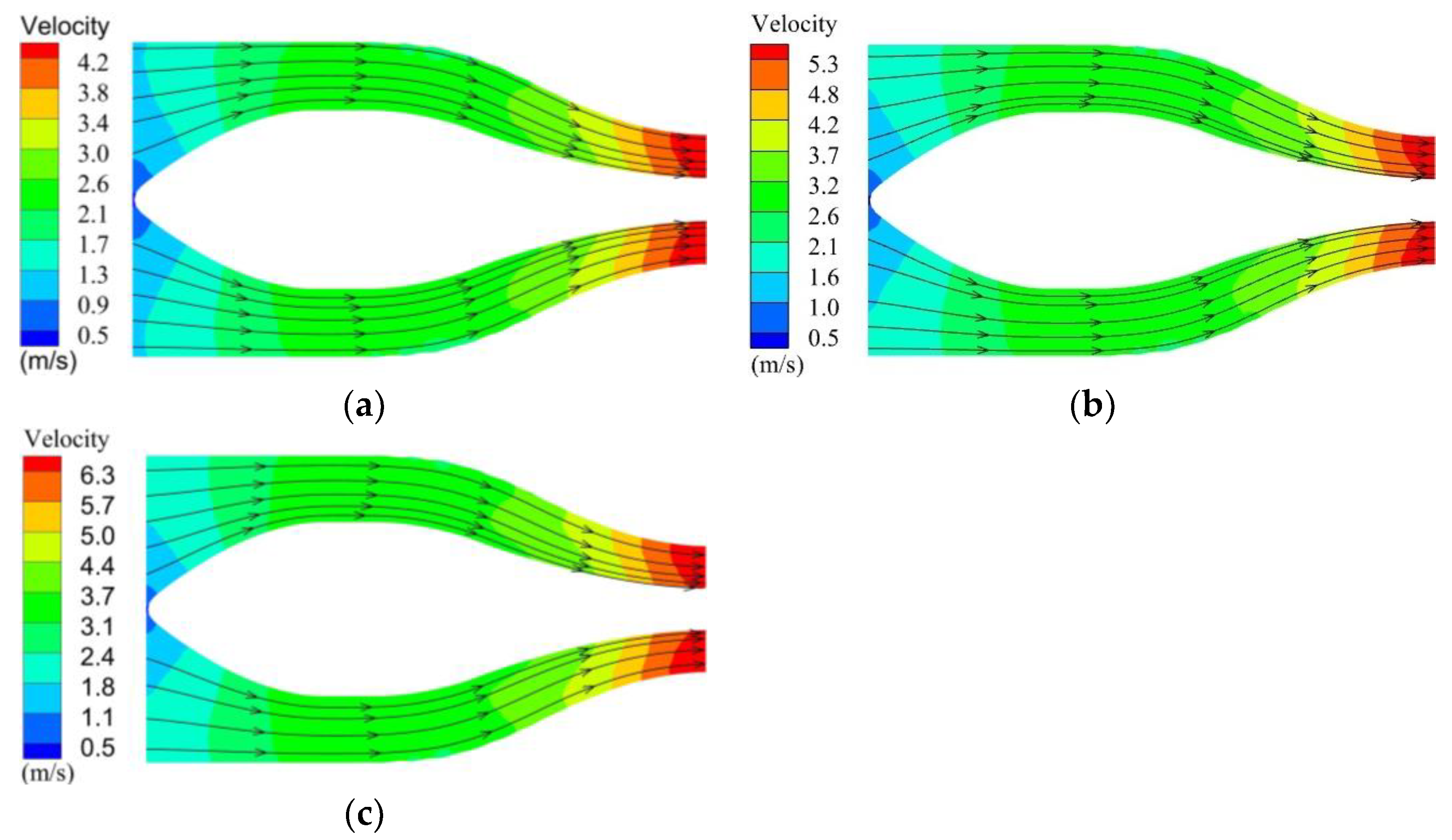
4.2. Hydraulic Performance of Inlet Passage

The hydraulic performance of the shaft tubular pump device was analyzed under three typical flow rate conditions: the small flow rate condition (Q = 0.8 Q_bep), the best efficiency condition (Q = 1.0 Q_bep), and the large flow rate condition (Q = 1.2 Q_bep). To further study the hydraulic performance of the inlet passage, the velocity distribution of cross-section under three typical conditions were selected to analyze. As shown in Figure 6, it was found that the velocity distribution was uniform, and the velocity increased gradually along the direction of the flow. In the shaft section, due to the small change of the area, the velocity changed slowly. Before the impeller chamber, the velocity of the water flow changed obviously due to the acceleration of section contraction. The flow velocity of the inlet passage outlet increased with the increase in the flow rate, and the flow was nearly perpendicular to the outlet section.

In this study, uniformity of the axial velocity distribution (V_u) and the weighted-velocity average angle (θ) were selected to conduct a quantitative analysis of the performance of the inlet passage. These two values are 100% and 90°, respectively, in the ideal state. The formulas are as follows:

$$V_u=[1-\frac{1}{\overline{u_a}}\sqrt{\frac{{\displaystyle \sum }{\left(u_{ai}-\overline{u_a}\right)}^2}{m}}]\times 100\%,$$

(7)

$$\theta =\frac{{\displaystyle \sum }{u}_{ai}(90°-{\tan }^{-1}\frac{u_{ti}}{u_{ai}})}{{\displaystyle \sum }{u}_{ai}},$$

(8)

where $\overline{u_a}$ and $u_{ai}$ represent axial velocity and averaged axial velocity, m/s, respectively; $u_{ti}$ represents the tangential velocity, m/s.

As shown in Figure 7, as the flow rate increased, both V_u and θ increased. When the flow rate was less than 1.0 Q_bep, the growth rate was greater than that under the large flow rate condition. When Q = 1.2 Q_bep, the V_u = 91.87%, which was 6.63% and 20.55% higher than that under 1.0 Q_bep and 0.8 Q_bep conditions, respectively, and θ = 87.63°, which was 2.43° and 8.69° higher than that under 1.0 Q_bep and 0.8 Q_bep conditions, respectively.

4.3. Hydraulic Performance of Impeller

In this study, the inlet of the impeller was 55 mm away from the center of the impeller. Figure 8 and Figure 9 show the velocity and pressure distribution of the impeller inlet, respectively. The law of velocity distribution was basically the same. The velocity decreased from the shroud to the hub, and there were three high-speed zones near the shroud. With the increase in the flow rate, the range of the high-speed zone was almost unchanged, while the low-speed zone near the hub gradually disappeared. The law of pressure distribution was almost the same. There were three high-pressure zones and three low-pressure zones, and the number of zones was the same as the number of blades. The pressure of the high-pressure zone decreased from the shroud to the hub, while the pressure of the low-pressure zone gradually increased from the shroud to the hub. The pressure of the impeller inlet section steadily declined as the flow rate increased, and the area of the high-pressure zone decreased while that of the low-pressure zone grew.

In order to observe the flow in the impeller chamber more clearly, the streamlines with different blade spanwise positions were analyzed. The diagram of different spans is shown in Figure 10. Since the flow pattern around each blade was essentially the same, only the flow pattern around a single blade is shown in Figure 11. As shown in Figure 11, when Q = 0.8 Q_bep, the flow near the hub at the outlet of the blade was deflected, and the flow was disordered. As the flow rate increased, the deflection of the water flow improved. When span = 0.5 and 0.9, the flow pattern in the impeller passage was smooth, without deflection or vortex, and the flow almost moved along the blade.

4.4. Hydraulic Performance of Guide Vane

The guide vane is behind the impeller, and its main function is to adjust the direction of the flow, which flows out from the impeller and takes the flow axially into the outlet passage. According to Figure 12, when Q = 0.8 Q_bep, the streamlines were disordered, and there was a vortex on the backside of the guide vanes. This shows that the guide vane had a poor adjustment effect on flow direction, which is not conducive to the recovery of circulation. When Q = 1.0 Q_bep, the flow in the guide vane was smooth, and the flow almost moved along the guide vane. When Q = 1.2 Q_bep, the flow pattern was basically the same as the optimal condition, while the streamlines on the guide blade working face were deflected.

The effect of the guide vane on water flow direction was evaluated by using the velocity circulation (Γ) of the outlet section; the expression of Γ is:

$$\Gamma ={{\displaystyle \oint }}_{L_1}{v}_{t}dL-{{\displaystyle \oint }}_{L_2}{v}_{t}dL={\displaystyle \iint }{\mathsf{\Omega }}_{x}dA,$$

(9)

where ${\mathsf{\Omega }}_x$ is the vorticity in the normal direction, s⁻¹, and A is area, m².

It can be found from Figure 13 that the Γ decreased with the increase in the flow rate, which indicates that the recovery effect of the guide vane is more obvious with the increase in the flow rate. The Γ= 0.68 m²/s under the optimal condition. When the Q = 0.8 Q_bep, the Γ= 1.46 m²/s, which is about 2.15 times of the optimal condition. When the Q = 1.2 Q_bep, the Γ= 0.31 m²/s, which is about 0.46 times of optimal condition.

4.5. Hydraulic Performance of Outlet Passage

As shown in Figure 14, in the outlet passage, the water diffused until it reached the outlet. When Q = 0.8 Q_bep, the adjustment effect of the guide vane was not obvious, and the water flow entered the outlet passage with obvious rotation. When Q = 1.0 Q_bep, the spiral motion of the flow in the outlet passage improved. As the flow rate continued to increase to 1.2 Q_bep, the streamlines were smooth, and the spiral motion almost disappeared. This was due to the circulation of guide vane outlet decreasing with the increase in the flow rate.

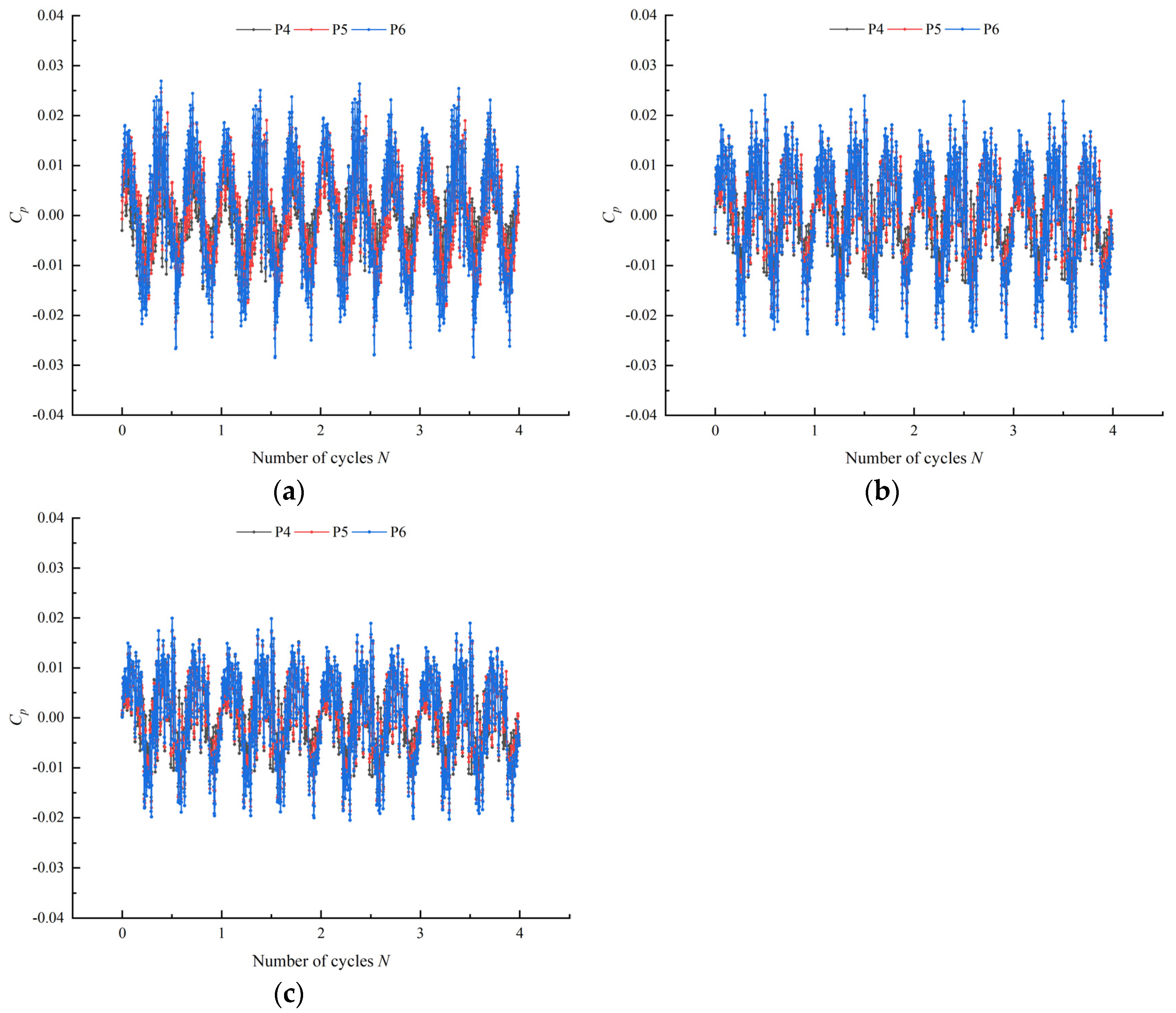
4.6. Pressure Pulsation

When the axial-flow pump device is operating, it produces dynamic pressure change with time. This phenomenon is known as pressure pulsation. In this numerical simulation, two sets of monitoring points were set at the impeller inlet and outlet, and the locations are shown in Figure 15. A total of eight cycles were calculated, and with the increase in rotation period, the calculation tended to be stable. To guarantee the reliability of the data, the last four cycles were selected for analysis. For better analysis, the pressure coefficient C_p was introduced:

$$C_p=\frac{p-\overline{p}}{0.5\rho u^2},$$

(10)

where p symbolizes the momentary pressure, Pa, $\overline{p}$ symbolizes the mean pressure over the cycle, Pa, and u is the impeller circumferential velocity, m/s.

Figure 16 and Figure 17 show the time domain at the impeller inlet and outlet. The pressure pulsation at P1-P6 shows obvious periodicity, and the change of pressure with time was sinusoidally distributed. Peaks and troughs appeared as many times as the number of blades in a cycle, indicating that the impeller rotation affects pressure pulsation. Furthermore, due to the effect of the guide vane at the same time, the fluctuation pattern at the outlet section was worse than at the inlet section. When Q = 0.8 Q_bep, the gap value of C_p at P1–P3 was 0.126, 0.202, and 0.244, respectively. When Q = 1.0 Q_bep, the gap value at P1–P3 was 0.105, 0.149, and 0.184, respectively. When Q = 1.2 Q_bep, the gap value at P1–P3 was 0.083, 0.137, and 0.176, respectively. When Q = 0.8 Q_bep, the gap value at P4-P6 was 0.046, 0.054, and 0.057, respectively. When Q = 1.0 Q_bep, the gap value at P4–P6 was 0.037, 0.041, and 0.049, respectively. When Q = 1.2 Q_bep, the gap value at P4–P6 was 0.032, 0.036, and 0.040, respectively. At the same flow rate, the pressure pulsation rose gradually along the radial direction in the same section, and that at the outlet section was significantly smaller than that at the inlet section. Furthermore, the pressure pulsation declined as the flow rate increased.

In this study, the rotating frequency (RF) was 24.17 Hz, and the blade passing frequency (BPF) was 72.5 Hz. To better understand the frequency distribution, the fast Fourier transform (FFT) was applied. The formula of the rotating frequency (RF) multiple is:

$$f_n=\frac{60F}{n},$$

(11)

where F symbolizes the frequency acquired by using the fast Fourier transform, Hz.

Figure 18 and Figure 19 show the frequency domain. The main frequency at P1–P6 was BPF, and the other harmonic frequencies were multiples of the BPF, indicating that the BPF determines the main frequency of pressure pulsation at the impeller inlet and outlet. The frequency distribution at the impeller outlet is more complicated. This is due to the dynamic and static interference between the impeller and guide vane. When Q = 0.8 Q_bep, the amplitude at the dominant frequency at P1–P3 was 0.062, 0.091, and 0.116, respectively; when Q = 1.0 Q_bep, the amplitude at P1-P3 was 0.039, 0.060, and 0.079, respectively; when Q = 1.2 Q_bep, the amplitude at P1–P3 was 0.034, 0.053, and 0.062, respectively. The amplitude at the small flow rate was about 1.5 times that at the optimal condition and about 2.01 times that at the large flow rate condition. Combining the above analyses, the inherent frequency of the pump device should not be close to BPF, in order to prevent resonance. In addition to this, the pump device should avoid operating under the small flow rate condition, in order to avoid blade damage due to severe pressure pulsation.

5. Conclusions

In this study, numerical simulation and a model test were carried out to reveal the variation law of hydraulic performance and pressure pulsation performance of the shaft tubular pump device with flow rate change. The liquid conveyed by the pump device in this study was water. The following conclusions were drawn:

• The external characteristic curves predicted by CFD were basically consistent with that obtained by the model test, indicating that the numerical simulation in this study has good reliability. For the well-designed shaft tubular pump device, the optimal efficiency reaches 76.52%. When Q = 0.8 Q_bep, the efficiency is 70.90%, and when Q = 1.2 Q_bep, the efficiency is 44.71%.
• The inlet passage has excellent hydraulic performance under different conditions; however, the flow pattern of the impeller and guide vane is disordered when the flow rate is low, and the guide vane has a poor adjustment effect on flow direction, resulting in an obvious spiral flow in the outlet passage. With the increase in the flow rate, the velocity circulation of the guide vane outlet decreases, and the spiral flow in the outlet passage is improved.
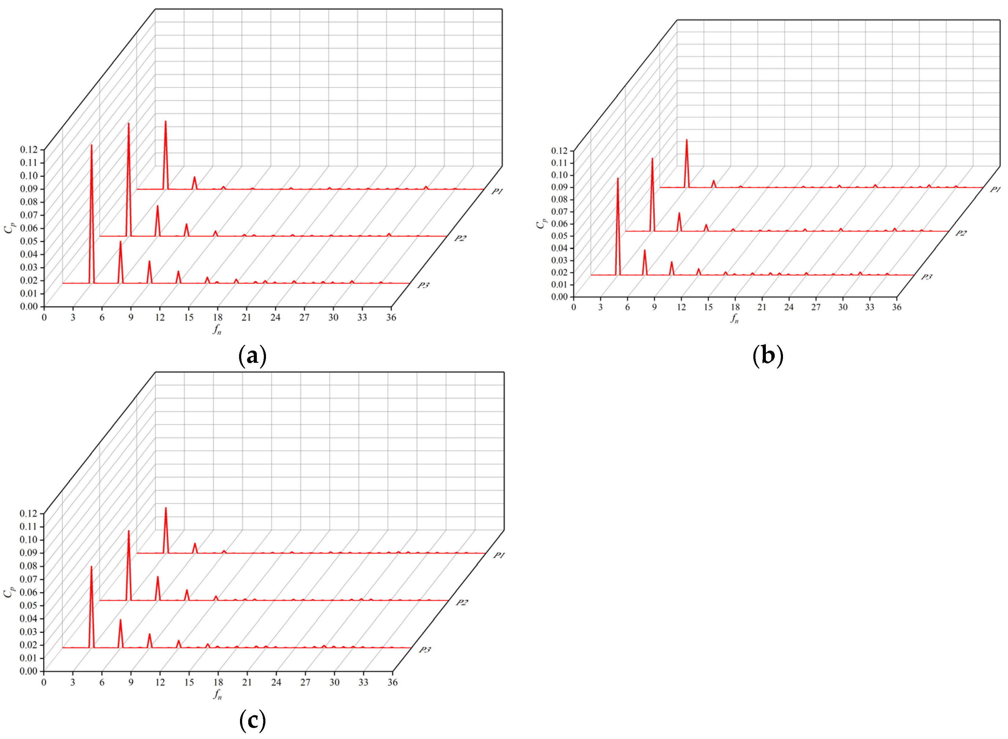
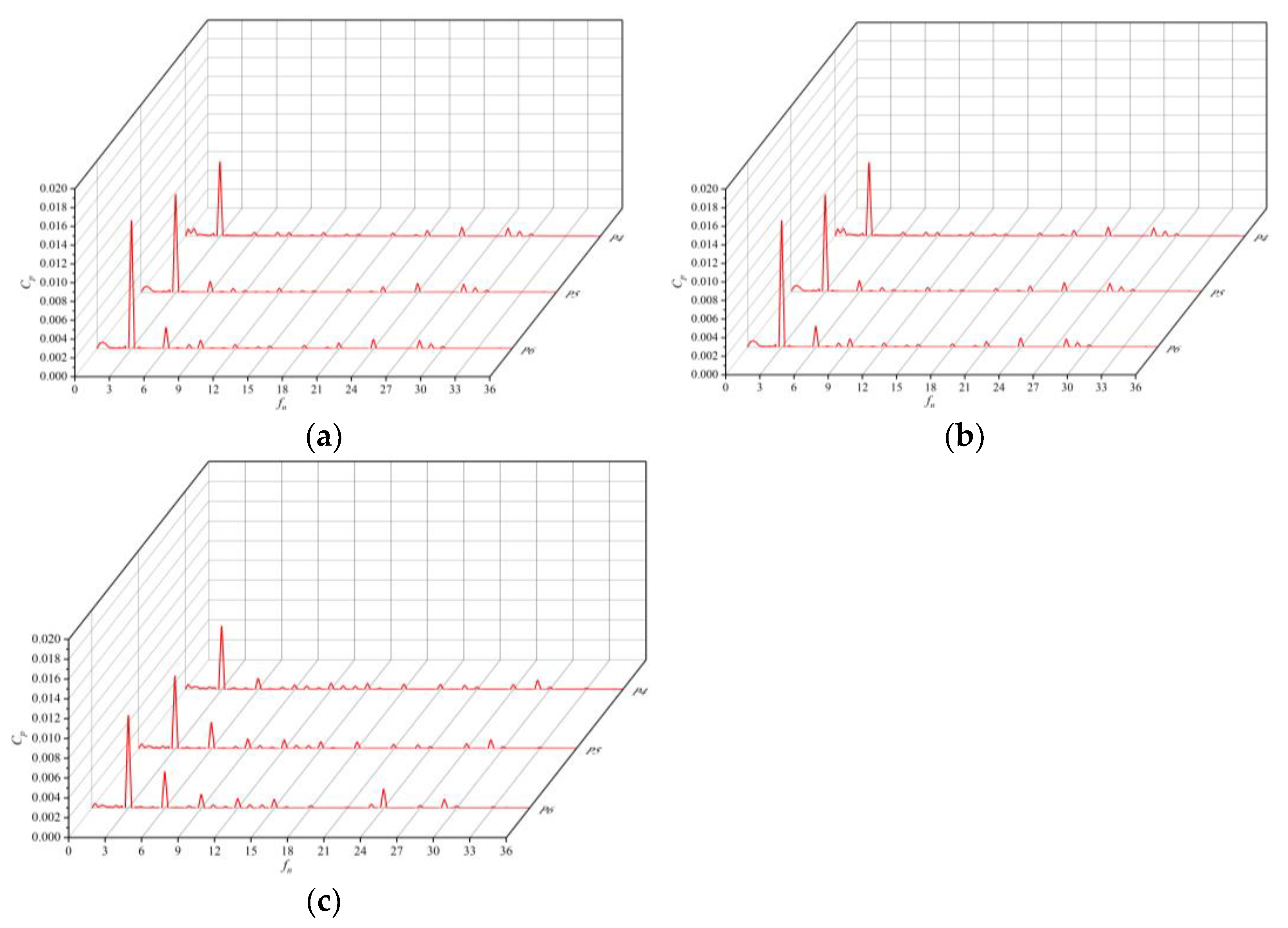
• The pressure pulsation of the impeller inlet and outlet has good periodicity, and the peaks and troughs occur as many times as the number of blades in a cycle. The BPF is the main frequency at the impeller inlet and outlet. This indicates that blade rotation is the main cause of pressure pulsation.
• At the same flow rate, the pressure pulsation rises gradually along the radial direction in the same section, and that at the impeller outlet is significantly smaller than that at the inlet section. Furthermore, the pressure pulsation declines as the flow rate increases. The amplitude at the small flow rate is about 1.5 times that at the optimal condition and about 2.01 times that at the large flow rate condition.
• In order to prevent resonance, the inherent frequency of the pump device should not be close to the blade passing frequency. Furthermore, the pump device should avoid operating under the condition of a flow rate of 0.8 Q_bep in order to prevent blade damage caused by excessive pressure pulsation.

References

1. Gomrokchi, A.U.; Rizi, A.P. Flexibility of energy and water management in pressurized irrigation systems using dynamic modeling of pump operation. Environ. Dev. Sustain. 2021, 23, 18232–18251. [Google Scholar] [CrossRef]
2. Gopal, C.; Mohanraj, M.; Chandramohan, P.; Chandrasekar, P. Renewable energy source water pumping systems–A literature review. Renew. Sustain. Energy Rev. 2013, 25, 351–370. [Google Scholar] [CrossRef]
3. Ji, D.; Lu, W.; Lu, L.; Xu, L.; Liu, J.; Shi, W.; Huang, G. Study on the comparison of the hydraulic performance and pressure pulsation characteristics of a shaft front-positioned and a shaft rear-positioned tubular pump devices. J. Mar. Sci. Eng. 2022, 10, 8. [Google Scholar] [CrossRef]
4. Cheng, K.; Li, S.; Cheng, L.; Sun, T.; Zhang, B.; Jiao, W. Experiment on Influence of Blade Angle on Hydraulic Characteristics of the Shaft Tubular Pumping Device. Processes 2022, 10, 590. [Google Scholar] [CrossRef]
5. Xu, L.; Lu, L.; Chen, W.; Wang, G. Study on comparison of hydraulic design schemes for shaft tubular pump device. J. Hydroelectr. Eng. 2011, 30, 207–215. [Google Scholar]
6. Lu, W.; Zhang, X. Research on model test of hydraulic characteristics for super-low head shaft-well tubular pump unit. J. Irrig. Drain. 2012, 31, 103–106. [Google Scholar]
7. Jiao, H.; Sun, C.; Chen, S. Analysis of the influence of inlet guide vanes on the performance of shaft tubular pumps. Shock. Vib. 2021, 2021, 5177313. [Google Scholar] [CrossRef]
8. Zhou, C.; Zhang, J.; Jiao, W.; Cheng, L.; Jiang, H. Numerical simulation of influence of shaft on performance of low head tubular pumping system. J. Drain. Irrig. Mach. Eng. 2021, 39, 231–237. [Google Scholar]
9. Xu, L.; Li, F.; Sun, S.; Ji, D.; Shi, W.; Lu, W.; Lu, L. Influence of outlet conduit parameters on the performance of shaft tubular pump. J. Drain. Irrig. Mach. Eng. 2021, 40, 73–78. [Google Scholar]
10. Guelich, J.; Bolleter, U. Pressure pulsation in centrifugal pumps. ASME J. Vib. Acoust. 1992, 114, 272–279. [Google Scholar] [CrossRef]
11. Barzdaitis, V.; Mazeika, P.; Vasylius, M.; Kartasovas, V.; Tadzijevas, A. Investigation of pressure pulsations in centrifugal pump system. J. Vibroengineering 2016, 18, 1849–1860. [Google Scholar]
12. Brennen, C. Hydrodynamics of Pumps; Concepts Nrec and Oxford University Press: Oxford, UK, 2011. [Google Scholar]
13. Wang, F.; Zhang, L.; Zhang, Z. Analysis on pressure fluctuation of unsteady flow in axial-flow pump. J. Hydraul. Eng. 2007, 38, 1003–1009. [Google Scholar]
14. Gonzalez, J.; Santolaria, C. Unsteady flow structure and global variables in a centrifugal pump. J. Fluids Eng. Trans. ASME 2006, 128, 937–946. [Google Scholar] [CrossRef]
15. Arndt, N.; Acosta, A.; Brennen, C. Rotor-Stator interaction in a diffuser pump. J. Turbomach. ASME 1989, 111, 213–221. [Google Scholar] [CrossRef]
16. Arndt, N.; Acosta, A.; Brennen, C. Experimental investigation of rotor-stator interaction in a centrifugal pump with several vaned diffusers. J. Turbomach. ASME 1990, 112, 98–108. [Google Scholar] [CrossRef]
17. Al-Obaidi, A.R. Analysis of the effect of various impeller blade angles on characteristic of the axial pump with pressure fluctuations based on time- and frequency-domain investigations. Iran. J. Sci. Technol.-Trans. Mech. Eng. 2021, 45, 441–459. [Google Scholar] [CrossRef]
18. Zhang, D.; Geng, L.; Shi, W.; Pan, D.; Wang, H. Experimental investigation on pressure fluctuation and vibration in axial-flow pump model. Trans. Chin. Soc. Agric. Mach. 2015, 46, 66–72. [Google Scholar]
19. Li, S.; Chen, S.; Zhou, Z.; Chen, J.; He, Z. Pressure fluctuation numerical simulation analysis of shaft tubular pump device. Water Resour. Power 2015, 33, 175–179. [Google Scholar]
20. Xu, L.; Karney, B.; Shi, W.; Ji, D.; Xu, B.; Lu, W. Influence of spiral flow on the hydraulic performance of a siphon outlet conduit in an axial flow pump system. J. Hydraul. Res. 2022, 60, 515–526. [Google Scholar] [CrossRef]
21. Kan, K.; Yang, Z.; Lyn, P.; Zheng, Y.; Shen, L. Numerical Study of Turbulent Flow past a Rotating Axial-Flow Pump Based on a Level-set Immersed Boundary Method. Renew. Energy 2021, 168, 960–971. [Google Scholar] [CrossRef]
22. Tremante, A.; Moreno, N.; Rey, R.; Noguera, R. Numerical turbulent simulation of the two-phase flow (liquid/gas) through a cascade of an axial pump. J. Fluids Eng.-Trans. ASME 2002, 124, 371–376. [Google Scholar] [CrossRef]
23. Kan, K.; Chen, H.; Zheng, Y.; Zhou, D.; Binama, M. Transient characteristics during power-off process in a shaft extension tubular pump by using a suitable numerical model. Renew. Energy 2021, 164, 109–121. [Google Scholar] [CrossRef]
24. Asim, T.; Mishra, R. Large-Eddy-Simulation-based analysis of complex flow structures within the volute of a vaneless centrifugal pump. Sadhana-Acad. Proc. Eng. Sci. 2017, 42, 505–516. [Google Scholar] [CrossRef] [Green Version]
25. Jafarzadeh, B.; Hajari, A.; Alishahi, M.; Akbari, M. The flow simulation of a low-specific-speed high-speed centrifugal pump. Appl. Math. Model. 2011, 35, 242–249. [Google Scholar] [CrossRef]
26. Ennouri, M.; Kanfoudi, H.; Taher, A.; Zgolli, R. Numerical flow simulation and cavitation prediction in a centrifugal pump using an SST-SAS turbulence model. J. Appl. Fluid Mech. 2019, 12, 25–39. [Google Scholar] [CrossRef]
27. Savar, M.; Kozmar, H.; Sutlovic, I. Improving centrifugal pump efficiency by impeller trimming. Desalination 2009, 249, 654–659. [Google Scholar] [CrossRef]
28. Sengpanich, K.; Bohez, E.L.; Thongkruer, P.; Sakulphan, K. New mode to operate centrifugal pump as impulse turbine. Renew. Energy 2019, 140, 983–993. [Google Scholar] [CrossRef]
29. Charles, H. Numerical Computation of Internal and External Flows; Wiley: Oxford, UK, 2007. [Google Scholar]
30. Wang, F. Analysis Method of Flow in Pumps and Pumping Stations; China Water Power Press: Beijing, China, 2019. [Google Scholar]
31. Shi, L.; Yuan, Y.; Jiao, H.; Tang, F.; Cheng, L.; Yang, F.; Jin, Y.; Zhu, J. Numerical investigation and experiment on pressure pulsation characteristics in a full tubular pump. Renew. Energy 2021, 163, 987–1000. [Google Scholar] [CrossRef]
32. Ramirez, R.; Avila, E.; Lopez, L.; Bula, A.; Forero, J. CFD characterization and optimization of the cavitation phenomenon in dredging centrifugal pumps. Alex. Eng. J. 2020, 59, 291–309. [Google Scholar] [CrossRef]
33. Zheng, Y.; Wang, K.; Lei, X.; Tang, F. 3D numerical simulation in inlet passages of pumping station by RNG k–ε turbulent model with wall-function law. Water Resour. Power 2008, 26, 123–125. [Google Scholar]
34. Xie, Y.; Ren, J.; Huang, H.; Zhang, X. Grid independence analysis of computational fluid dynamics based on chi-square test. Sci. Technol. Eng. 2020, 20, 123–127. [Google Scholar]
Figure 1. Three-dimensional model.
Jmse 10 00750 g001
Figure 2. Grid independence analysis.
Jmse 10 00750 g002
Figure 3. Grid diagram: (a) inlet passage; (b) outlet passage; (c) impeller; (d) guide vane.
Jmse 10 00750 g003
Figure 4. Physical diagrams of test: (a) pump device; (b) impeller; (c) guide vane.
Jmse 10 00750 g004
Figure 5. Comparison of external characteristics between numerical simulation and tests.
Jmse 10 00750 g005
Figure 6. Velocity distribution of cross-section in inlet passage: (a) Q = 0.8 Qbep; (b) Q = 1.0 Qbep; (c) Q = 1.2 Qbep.
Jmse 10 00750 g006
Figure 7. Vu and θ of the inlet passage outlet section.
Jmse 10 00750 g007
Figure 8. Velocity distribution of impeller inlet: (a) Q = 0.8 Qbep; (b) Q = 1.0 Qbep; (c) Q = 1.2 Qbep.
Jmse 10 00750 g008
Figure 9. Pressure distribution of impeller inlet: (a) Q = 0.8 Qbep; (b) Q = 1.0 Qbep; (c) Q = 1.2 Qbep.
Jmse 10 00750 g009
Figure 10. Diagram of different spans.
Jmse 10 00750 g010
Figure 11. Flow pattern of the impeller: (a) span = 0.1 (near the hub); (b) span = 0.5; (c) span = 0.9 (near the shroud). In each picture, there are impeller inlets at the bottom and impeller outlets at the top.
Jmse 10 00750 g011
Figure 12. Three-dimensional streamlines diagram of guide vane: (a) Q = 0.8 Qbep; (b) Q = 1.0 Qbep; (c) Q = 1.2 Qbep.
Jmse 10 00750 g012
Figure 13. The velocity circulation of guide vane outlet.
Jmse 10 00750 g013
Figure 14. Three-dimensional streamlines of pump device: (a) Q = 0.8 Qbep; (b) Q = 1.0 Qbep; (c) Q = 1.2 Qbep.
Jmse 10 00750 g014aJmse 10 00750 g014b
Figure 15. Arrangement of pressure monitoring points.
Jmse 10 00750 g015
Figure 16. Time domain diagram of Cp at impeller inlet: (a) Q = 0.8 Qbep; (b) Q = 1.0 Qbep; (c) Q = 1.2 Qbep.
Jmse 10 00750 g016
Figure 17. Time domain diagram of Cp at impeller outlet: (a) Q = 0.8 Qbep; (b) Q = 1.0 Qbep; (c) Q = 1.2 Qbep.
Jmse 10 00750 g017
Figure 18. Frequency domain diagram of Cp at impeller inlet: (a) Q = 0.8 Qbep; (b) Q = 1.0 Qbep; (c) Q = 1.2 Qbep.
Jmse 10 00750 g018
Figure 19. Frequency domain diagram of Cp at impeller outlet: (a) Q = 0.8 Qbep; (b) Q = 1.0 Qbep; (c) Q = 1.2 Qbep.
Jmse 10 00750 g019