Article

Extreme Wind Wave Climate off Jeddah Coast, the Red Sea

Faculty of Maritimes Studies, King Abdulaziz University, Jeddah P.O. Box 80401, Saudi Arabia
*
Author to whom correspondence should be addressed.
J. Mar. Sci. Eng. 2022, 10(6), 748; https://doi.org/10.3390/jmse10060748
Submission received: 31 March 2022 / Revised: 20 May 2022 / Accepted: 25 May 2022 / Published: 29 May 2022

Abstract

:
Climate change can give rise to significant changes in the intensity and frequency of extreme events. In the present study, extreme wave events off the central-eastern coast of the Red Sea, near the city of Jeddah, were investigated using a 39-year wave hindcast generated using WaveWatch III configured at a 3.3 km resolution forced with ERA5 reanalysis winds. The validated model outputs were used to derive the annual and seasonal climatology for the region at a few selected locations off the Jeddah coast. The study revealed robust temporal and spatial variability in the region, considering the influence of both northern and southern Red Sea waves that meet at the convergent zone. Generalized Pareto Distribution (GPD) and Generalized Extreme Value (GEV) were two models used for the estimation of extreme wave analysis in the study region. The extreme significant wave heights were estimated for 10, 25, 50, and 100-year return periods. For offshore locations, the estimated return periods using the GPD method were 3.27, 3.44, and 3.38 m, respectively. GPD with the POT method was the more suitable approach, as it produced reduced bias and RMSE. At all locations, linear trends show an increase during the summer, winter, and pre-summer periods. No significant increase in the Hs trend was observed at the selected locations near and off the coast. However, the decrease in trend observed at all locations during the pre-winter period was noticeable for the 99th percentile Hs.

1. Introduction

An understanding of future extreme conditions is crucial for the construction of reliable and effective coastal defense infrastructure; coastal and ocean engineering design and operation [1,2,3]. Extreme wave analysis is also more crucial in the deep understanding of coastal dynamics and the development design of sustainable, low-impact coastal protection measures. Further, this will bring out clear insight into the region and site specific characterization studies [4]. Awareness of extreme wave conditions is very important for the scientific community, industry, government and coastal engineering sectors, and others. Data regarding the most severe wave conditions can be used to analyse the withstand capacity of coastal and offshore structures. Wave studies have generally concentrated on describing the spatiotemporal variabilities of wave heights as well as establishing wave heights in order to inform structural design in the field of ocean and coastal engineering. Typically, most coastal and off shore structures are built to resist strong wave climates to a specific return level. Many statistical studies have been used in the fields of marine and atmosphere science [5,6,7,8,9]. For proper assessment of the return period values, extreme value analysis (EVA) over a comparatively longer period is required [10,11,12,13]. The estimation of the return period requires past decades’ time series wave data for statistical analysis. The pre-recorded buoy data, satellite data, re-analysis data, etc., can be used for statistical analysis. The return period is calculated using a statistical study of historical wave height time series. Data from a wide range of sources, including satellite altimetry, re-analysis or hindcast datasets, and in situ buoy observations may differ. Long-term changing trends in wave heights in diverse ocean scenario regions can be unravelled using regression analysis, empirical cumulative distribution function approach technique, and using wave hind cast and re-analysis data [14,15,16,17,18,19,20,21].
The length of the time series record of significant wave height (Hs) is the main factor when considering the extreme value analysis of waves. The most accurate information would be from a wave rider buoy, whereas the difficulty of getting such a long period measurement for a particular region of interest is complemented by using the validated numerical model hindcast results. Recent hindcasts of the ocean give better quality results [22] as the input fields are significantly improved with the adoption of more data assimilation into the model.
Many studies have been carried out by researchers to improve the accuracy and prediction of waves in the Red Sea [20,23,24,25,26,27]. Most of these studies provide a better understanding of the wave climate of the Red Sea. Shanas et al. [21] detailed the wave characteristics and distribution of wind waves covering a period of 32 years from hindcast data produced with a numerical spectral wave model. The climatology of the area suggests that the Red Sea shows a distinct zone with contrasting trends in the wind waves. The role of climate indices, trends, and variability of wind waves are detailed. Moreover, studies representing the seasonal characteristics of waves, including circulation, have been discussed in the literature [20,21,23]. To improve the precision of wave prediction in the Red Sea, Langodan et al. [24] proposed modifying the source term.
Only a few studies have taken place off the Jeddah coast. Refs. [27,28] used model results to distribute wind waves along the coast. The spectral wave characteristics along the Jeddah coast were investigated by Shanas et al. [29]. The superimposition of wind, sea, and swell has been examined, as well as notable general features like diurnal variations. Along the Jeddah coast, waves are mostly observed between the west and northwest [27]. Alaa and Aboobacker [30] addressed the spectral characteristics of the near coast of Jeddah using SWAN modelling. Seasonal monthly and diurnal characteristics were detailed in the study.
An extreme value analysis of wind waves on the eastern coast of the Red Sea was performed by Langodan et al. [31]. The study is mostly based on the extreme wave analysis of a reef-protected coastal zone using a 30-year model hindcast. A similar study has been reported along the Island-protected southern coast of the Red Sea [32]. The study investigated the extreme wave conditions in the Island protected area where the Indian monsoon and local climate interact. Furthermore, due to the complex bathymetry and the shallowing effect caused by the presence of coral reefs, the wave conditions in this region are more complex.
The goal of our present study is to look at the extreme wave heights off the Jeddah coast and near the Jeddah port on the western coast of Saudi Arabia (Figure 1) as well as investigate the various methods for incorporating the rise in extreme value evaluations used in coastal hazard and coastal engineering applications, especially in the port area. The trend analysis and climatology for off shore intermediate and shallow water depths need to investigate for further understanding of the wind waves in the region from a climatological perspective. Limited research on wave climate off the Jeddah coast has been conducted in the absence of long-term wind wave data. The northern Red Sea and the southern Red Sea are two separate regional divisions with 32-year-long numerical simulations based on various wave climatological perspectives [21]. Jeddah is in the central part of the Red Sea connecting the northern and southern regions, making it geographically important in the climate transition between the regions. Considering the scarcity of data, this study can be considered the baseline study for the Red Sea coast. This method can be applied wherever applicable with a limited number of data.

2. Study Area

The Red Sea extends from 12.5° to 30° N latitude, connecting to the Indian Ocean through the Bab-el-Mandeb Strait to the south. The Jeddah coast is located in the central Red Sea between 21.55° N and 21.85° N, and 38.9° E and 39.3° E (Figure 1). The predominant direction of Red Sea winds is NNW and are present throughout the year. The intensity of winds in the winter is relatively higher compared to that of the summer. South of the Jeddah coast is a convergent zone of winds [33]. The central-eastern coast of the Red Sea, which includes Jeddah, is characterized by wind waves from both the northern and southern Red Sea. The superimposition of wind waves and the interaction of multi-directional waves are present [30].
We have selected eight locations (Station1 (St8) to Station8 (St8)) off the Jeddah coast to conduct extreme value analysis. Two of these locations are near the coast, three are at intermediate distances, and the remaining three are further offshore (Figure 1). The points are considered in such a way to understand the climatology of the waves at both deep water intermediate and shallow water stretch covering the domain.

3. Data and Methodology

3.1. Model Description: Computational Grid and Bathymetry

The spectral numerical wave model WaveWatch3 (hereafter WW3) was implemented in wind wave simulation for the entire Red Sea. We followed the approach of Shanas et al. (2017 (b)) for simulation with the input parameterization scheme of ST4 physics applied. The ST4 physics [34] gives better results in the Red Sea [21,23]. The dissipation scheme for the source term is used in the model proposed by Bidlot et al. [35]. The model run was performed for a period of 39 years from 1979 to 2018 on HPC. The regional model entails the entire Red Sea with a geographic coverage between 12° and 30° N as well as 32° and 44° E. The model was implemented with a horizontal resolution of 3.3 km. The most recent updated version of GEBCO, with a spatial sampling interval of 15 arcs second data, was used for the bathymetry.
Although many islands are present all along the Red Sea coast, anything less than the grid resolution was ignored as a wet grid. The model started with a calm condition similar to that implemented by Shanas et al. [29] and Langodan et al. [24].

3.2. Input Data Generation Boundary Condition

The wave model was driven by ERA5 wind velocity components at 10 m intervals available at the European Centre for Mesoscale Weather Forecasts (ECMWF), which provides an hourly temporal scale with a spatial resolution of 0.25 km for the period between 1979–2018. Recently updated bathymetry from the GEBCO 2019 database [36] was used for the model simulation. Both latitude and longitude have a resolution of 15 arc seconds. Water level, currents, and ice impact are not activated. For the discretization of the energy spectrum, the wave model is set up with a 3.3 km grid spacing encompassing the entire Red Sea domain, with 33 directions and 30 frequencies starting at a 0.04 Hz geometric step of 1.1. The 39-year model outputs of wave parameters (significant wave height, mean wave direction, mean wave period) are stored in steps of 3 h between 1979–2018.

3.3. Model Validation

Measurements in the Red Sea region are very sparse. The only available wave measurement in the Red Sea is located off THUWAL at around 700 m in water depth. The data consists of 2-year measurements between October 2008 and November 2010 [37]. The details of the wave buoy data can be found in Ralston et al. [25] and Langodan et al. [24].
The time series and scatter plot between the measured and modelled output at the buoy location is shown in Figure 2. The model gives reasonable agreement with the measured data with a correlation coefficient of 0.91 and a bias value of 0.25. The Root Mean squared Error (RMSE) between the measured and model output is at the lower side (<0.3 m), suggesting the performance of the model is satisfactory. Moreover, the high peaks during the data period are reproduced satisfactorily, showing the improved accuracy of the model in picking up the higher events. The comparison statistics are inconsistent with Shanas et al. [21] had compared the model output at the same location.

Point Selection for the Extreme Value Analysis

Considering the influence of the nearshore complex region and the relative importance of the economic zone of the Jeddah coast, eight points were randomly chosen to cover nearshore, intermediate, and offshore water depths. The extreme value analysis was performed based on the 3 h model output extracted at the selected location between 1979–2018. The table below (Table 1) shows the coordinates and duration of extracted data at eight locations. Figure 3 shows the capability plot for the eight selected locations with the normal distribution of monthly maximum data at each location.

4. Extreme Value Analysis
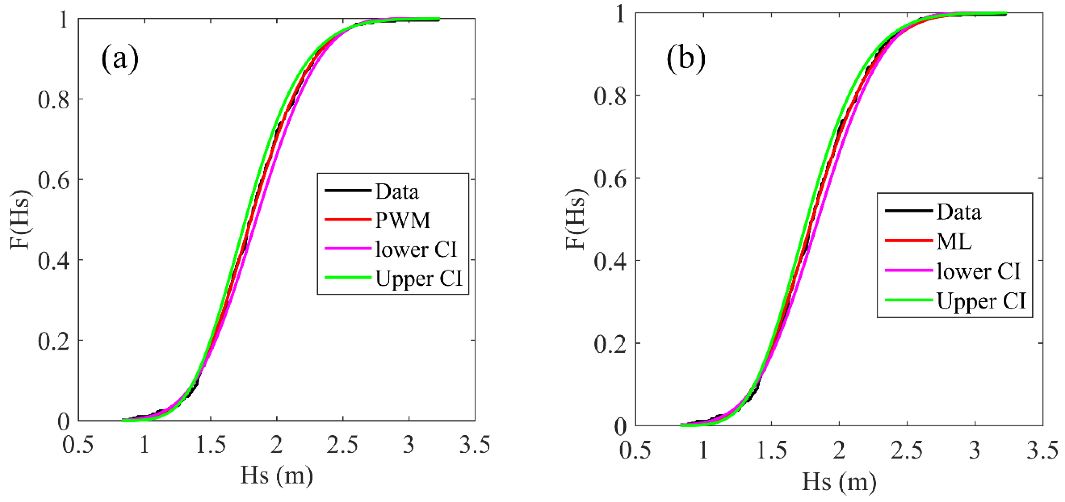
Statistical modelling is an important tool in coastal engineering and design applications. Specifically, extreme value analysis is a well-known methodology applied in various fields of science, including engineering and oceanography, in order to find out the probability of extreme events from the observed or measured data [38]. The two most common and widely used approaches for the estimation of wind waves are generalized extreme value (GEV) and generalized Pareto distribution (GPD) [39,40]. Extreme value analysis is generally carried out using the most traditional methods, such as the initial distribution method (IDM), annual maxima (AM) method, and peak over threshold (POT). These three methods differ in the preparation of sample data. The first method uses all the recorded data available for a period and applies a cumulative distribution to this data. For AM and POT, only the peaks are considered. For the AM method, the typical block maxima chosen is one year [41], while the POT method considers local maxima or storm peaks above a chosen threshold. The most important aspect of extreme value analysis is the proper selection of data. In the Red Sea, the interaction between multiple directions of waves is possible [23,24]. As a result, the wave environments of the Red Sea are described as having a mixed distribution.
For the estimation of the return period, we have analysed both the GEV and GPD methods. The maximum likelihood estimate (ML) approach and the probability-weighted moments (PWM) method were used to fit the model (PWM). The WAFO toolbox was used to perform distribution fitting and the estimation of parameters [42].

4.1. GEV Method

For a random variable, the GEV distribution of significant wave height ( H s ) has the cumulative distribution function (CDF) as:
G E V ( H s ; μ ; σ ; δ ) = { exp ( ( 1 + δ ( H s μ σ ) ) 1 δ )   f o r   δ 0 exp ( exp ( ( ( H s μ ) σ ) ) )   f o r   δ = 0
where, μ = l o c a t i o n , σ  = scale, and δ  = shape, these are the parameters of the distribution and which fall in the range of < μ < ,   σ > 0, and < δ < , by analyzing the shape parameter, δ , one can obtain Gumbel ( δ = 0, Fréchet ( δ > 0) and Weibull ( δ < 0) distribution.
Then the returned period ( H p ) can be estimated as:
H p = { μ σ δ   ( 1 ( l o g ( 1 1 T ) ) δ )   f o r   δ 0 μ σ   ln ( l o g ( 1 1 T ) )   f o r   δ = 0

4.2. GPD Method

The CDF for GPD is given as:
G P D ( H s ; μ ; σ ; δ ) = { 1 ( 1 δ ( H s μ σ ) ) 1 δ   f o r   δ 0 1 exp ( ( H s μ σ ) )   f o r   δ = 0
The range of parameters are < μ < ,   σ > 0 and of < δ < .
Then, using the GPD distribution model, the returning period ( H p ) can be estimated as follows:
H p = {   μ + σ δ   ( ( λ T ) δ 1 )   f o r   δ 0 μ + σ   ln ( λ T )   f o r   δ = 0
where,   λ = N u N T , N u is the total number of exceedances beyond the chosen threshold μ 0 , and NT is the number of years in the record.

4.3. Threshold Selection for GPD

The value of the threshold, time span, and minimum time span are key parameters in the POT method and can have a considerable impact on the frequency and exceedance estimations [39]. To make sure that the selected time span includes sufficiently-resolved independent storms, the timespan (Δt) should be chosen wisely. Different ranges of Δt can be found in the literature [39]. In this analysis, a Δt of 5 is used for the POT method.
The threshold selection significantly influences the return level estimates. The selected threshold should not be too large or too low, since the chance of uncertainties in the estimated parameters could be high and results might produce a high variance. If we set the threshold so high that only a few exceedances occur, the analysis is unlikely to produce any relevant results. The analysis of the data derived from GPD will only be reliable if the threshold is set so low to the point that most of the data points are exceedances.
As a result, a sensible strategy is required for the fitting of these exceedances to the threshold in a satisfactory manner, considering the EVA model and the lowest threshold as possible. Different methods exist for threshold selection. The dispersion index method and the mean residual life method are two common ones. The dispersion index consists of the ratio between the expected number of peaks and variance, which may be used to identify clusters and confirm the Poisson character. This ratio equals a value of one for a Poisson distribution. The dispersion index should be near a value of one for an acceptable peak separation [42]. Plotting the ‘mean excess’ against Hs for a range of Hs is the Mean residual life (MRL) method [38]. Lines with a 95% CI are given here as well. Above the threshold, when the GPD model becomes valid, the plot should be linear. In this study, we used the dispersion index method to select the mean excess method, which provides consistent estimates and a good number of independent high events (Figure 4).

5. Results and Discussions

5.1. General Wave Characteristics from Model Outputs

Figure 5 shows the time series significant wave height at each station from 1979–2018. The mean wave height of the region is around 0.7 m for locations 1–3, 0.6 m for locations 4–6, and the nearshore wave height is around 0.25 m. The maximum wave height reported at the present study location was 3.31 m at station 3. The second maximum was 3.26 m reported at station 2. Statistical analysis was carried out using seasonal characteristics. Generally, the wind waves are NNW dominant throughout the year on the central coast of the Red Sea [23,24]. There exists a convergent zone just south of the Jeddah area which may extend up to 21.5° N [25]. The consistent summer-winter convergence may have a profound influence on the average climate of the area under study. The monthly maximum wave height would clearly show this variation. For instance, although the predominant waves (more than 80%) are from the NNW, the maximum wave height is not associated with a NNW direction. In fact, this happened during the winter period. At locations 1–3 and 6–8, the maximum wave height was observed during December 1985. This is associated with extremely high waves that are generated from the southern Red Sea and propagated into the northern Red Sea.

5.2. Annual Climatology

This study presents the comprehensive wave climatology off the coast of Jeddah, based on a 39-year hindcast created using WAVEWATCH III built on a 3.3 km resolution grid. Figure 6 shows the annual climatology of the study area from 1979–2018. The significant role of wind inputs from the southern and northern Red Sea areas is seen in the overall distribution of mean Hs values in most parts of the Jeddah basin. The Tokar Gap winds [25,43] play a prominent role in the extreme wave height off the Jeddah coast. The annual climatology of the study area from 1979–2018 (Figure 6) also indicates the extreme waves distributed along the central part of the Red Sea, which is also reflected off the Jeddah coast. This highest distribution of wave height measured in the central Red Sea may be due to the superimposed northerly and southerly wave events. During the pre-winter and winter seasons, the distribution mean Hs in Jeddah’s nearshore region is lower than further offshore, but the distribution mean Hs in the nearshore area is comparatively high during the pre-summer and summer seasons. As seen in the wave rose diagram of the study area for the 1979–2018 period (Figure 7), the waves off the Jeddah coast are predominantly from the NW. The analysis shows that moderate wave conditions with significant wave heights less than 1 m frequently affect the study area, especially in the nearshore area and mainly from the NW. In the nearshore area (locations 7 and 8), the waves come from the NNW with moderate frequencies. However, in the offshore area (locations 4–6), significant wave heights less than 1.5 m propagating from the S with less frequency indicate the influence of a southerly wave event.

5.3. Seasonal Climatology

The seasonal climatology of wind waves in the Jeddah region is shown in Figure 8. The seasonal climatology depicts that the Jeddah region experiences slightly higher wave heights during the winter compared to other seasons. The wave heights are the least during the pre-winter period. It is worth noting that the predominant direction of wind waves is from the NNW direction at all locations (Figure 8). More than 90% of the waves are reaching from the NNW direction, whereas the contribution of waves from the southern Red Se is much less compared to the NNW swells that reach the region. Ref. [23] reported that the highest significant waves in the Red Sea are mostly distributed in the central region and gradually decrease towards the northern and southern Red Sea basins. Considering the climatic condition and the basin-wide scale atmospheric circulation, the probability of the formation of a tropical cyclone in the Red Sea is negligible. Hardly any cyclone events have been reported. Hence, the extreme events or the higher waves in this region are mostly associated with the wind sea dominant region. The most intense waves are those generated in the Tokar Gap [24].

5.4. Trend Analysis

The trend analysis of long term climatological times series can be estimated using either the linear or non-linear parametric method. For the parametric method, the date needs to be normally distributed and independent whereas, in the non-parametric trend test, it is not necessary to be normally distributed. The Mann-Kendall trend test is one of the non-parametric trend tests. Mann-Kendall trend test was performed for the time-series data at the selected location for the period of 1979–2018. For estimating trends, the method adopts Sen’s slope method [44,45,46]. The non-parametric trend-based estimates allow for more advantages over the traditional linear trend estimates. The wind-wave climatology for the selected location around the Jeddah coast was investigated. The maximum 90th percentile and 99th percentile values of Hs with the Mann-Kendall estimated trend are shown in Figure 9. The table below (Table 2) shows the Mann Kendal estimated trend of Hs at the eight locations.

5.4.1. Seasonal Trend

To examine the seasonal variability in wave height, trend analysis at seasonal scales was performed on the 99th percentile and 90th percentile Hs values through the Mann-Kendall trend test (Figure 9). Moreover, an increase/decrease in trend was estimated using the Theil-Sen estimator. It is evident that for most of the season at all locations, the magnitude of Hs is in an increasing trend. This can be observed during winter, summer, and pre-summer periods. However, the decrease in trend observed at all locations during the pre-winter period was noticeable for the 99th percentile Hs. In fact, the decrease in Hs trend during the pre-winter 90th percentile of Hs was observed only at location 1 and 3. At the nearshore location, location 7 and 8, the Hs shows an increasing trend except during the summer and pre-winter periods.

5.4.2. Extreme Wave Analysis
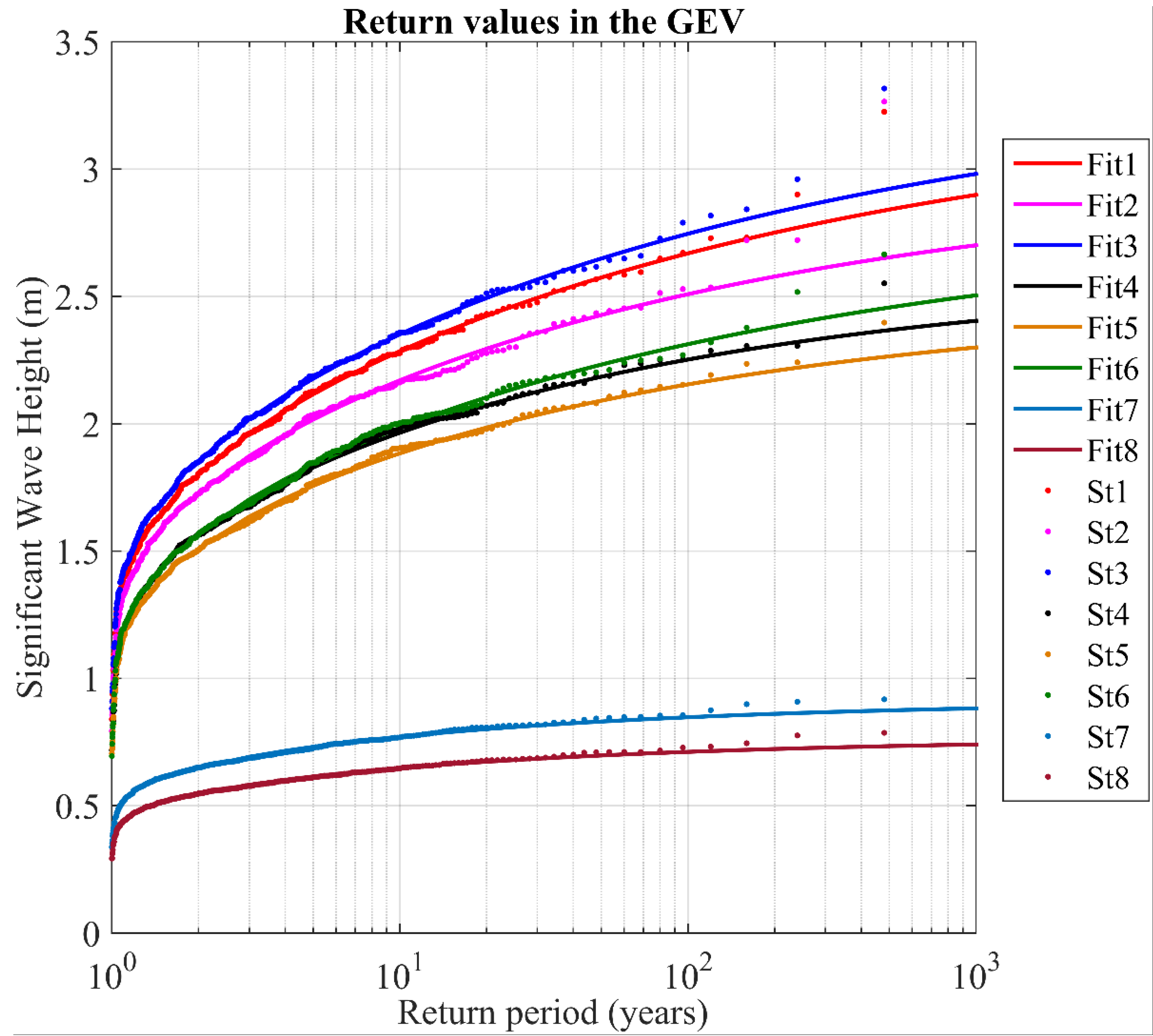
The extreme value analysis of Hs between 1979 and 2018 was carried out at the selected location. We tested both GEV and POT analyses. For the GEV analysis, GEV distribution was carried out using the data fitted to annual maxima, monthly max, daily maxima, etc. Here, we have carried out the analysis based on the monthly and annual maxima data. The estimation of the parameter was performed by the PWM method ad ML method. The CDF plots for GEV distribution for annual and maximum block method at the St1 location is shown in Figure 10 and Figure 11, and the estimated parameter based on the PWM method for GEV is shown in Table 3.
The RMSE between the fitted distribution and the empirical cumulative distribution obtained from the data should be close to zero for a reliable estimate of the return period (Figure 10 and Figure 11). The ML method yields better results for the location in this study. This is consistent with Langodan et al. [31], who found the ML method more suitable for the study area north of the Jeddah coast.
For reliable estimates of the extreme value analysis in regards to GPD, the selection of a suitable threshold value is necessary. Following the mean excess method, the threshold values selected for all locations were high enough for observations to be independent and converge the POT analysis into GPD. The RMSE for the estimated CDF is shown in the table. Using the threshold obtained from the mean excess method, the data is fitted to the GPD distribution. The corresponding PDF plots for GPD analysis are shown in Figure 12.

5.5. Return Period

Table 4 and Table 5 show the estimated return period for the study area at all locations for 10, 25, 50, and 100 years for GEV (annual and monthly) and GPD (POT method). From the estimated return level of Hs at 100 years, the offshore locations with Hs of 3.01, 2.66, and 3.10 m for GEV (monthly maximum) and 3.27, 3.44, and 3.38 m for GPD, respectively. It is evident that the maximum of the simulated data is higher than the estimated GEV return value, even for the 100-year return period. Even though the data is fitted with less RMSE, the discrepancies in the maximum return value should be noted. The limitation of the GEV method is that it doesn’t use all the information in the observed data. In turn, this introduces uncertainty in the estimated return value, whereas the GPD estimates and maximum simulated data are closer and more reliable. The RMSE between the EDF is also relatively lower for the GPD method, suggesting better reliability for the estimated return period. Figure 13 and Figure 14 show the return period estimated for the GEV and GPD methods.

6. Conclusions

Wind wave characteristics in the Red Sea are complex mostly related to prevailing wind systems. The superimposition swells systems and the interaction of NNW- and SSE-generated waves may cause a large amount of variability in the nearshore climate of the Red Sea coast. Considering recent active developments and the economic importance of the Jeddah coast of the central eastern coast of the Red Sea, an investigation of the extreme wave analysis has been performed based on the 39 year numerical modelling results. The WW3 model was simulated for a period of 39 years from 1979–2018. The extracted output at selected locations off the coast was used for the extreme value analysis and to understand climate and trend variability. The validated model outputs were used to derive the annual, and seasonal climatology for the region. The study reveals robust temporal and spatial variability in the region, considering the influence of both northern and southern Red Sea waves to meet the convergent zone. The two models used for the estimate of the extreme wave analysis for the study region were the Generalized Extreme Value (GEV) and the Generalized Pareto Distribution (GPD). The extreme significant wave heights were estimated for 10, 25, 50, and 100-year return periods. The GPD and POT techniques were a better fit for the study area since they reduce bias and RMSE. Using trend analysis, it is evident that during most seasons at all locations, the magnitude of Hs is in an increasing trend. This can be observed during the winter, summer, and pre-summer periods. However, the decrease in trend observed at all locations during the pre-winter period is noticeable for 99th percentile Hs.

Author Contributions

Conceptualization; methodology; software, S.V. and F.A. Wrote the manuscript with the support from F.A. and S.V., and F.A. contributed to writing—review and editing. F.A. supervised the whole project. All authors have read and agreed to the published version of the manuscript.

Funding

This research was funded by the Deanship of Scientific Research (DSR), King Abdulaziz University, Jeddah, under grant No. G-306-980-1441.

Institutional Review Board Statement

Not applicable.

Informed Consent Statement

Not applicable.

Data Availability Statement

Not applicable.

Acknowledgments

The author, therefore, gratefully acknowledges DSR’s technical and financial support. Thanks to Dean, Faculty of Maritime Studies, King Abdulaziz. The simulations in this work were performed at King Abdulaziz University’s High-Performance Computing Center (Aziz Supercomputer) (http://hpc.kau.edu.sa), accessed date: 1 October 2021 to 31 October 2021).

Conflicts of Interest

The authors declare no conflict of interest. The funders had no role in the design of the study; in the collection, analyses, or interpretation of data; in the writing of the manuscript; or in the decision to publish the results.

References

  1. Vanem, E.; Fazeres-Ferradosa, T.; Rosa-Santos, P.; Taveira-Pinto, F. Statistical Description and Modelling of Extreme Ocean Wave Conditions. Proc. Inst. Civ. Eng.-Marit. Eng. 2019, 172, 124–132. [Google Scholar] [CrossRef]
  2. Taveira-Pinto, F.; Rosa-Santos, P.; Fazeres-Ferradosa, F. Integrated management and planning of coastal zones in CPLP—Part 1 [Gestão e planeamento integrado das zonas costeiras da CPLP—Parte 1]. J. Integr. Coast. Zone Manag. 2020, 20, 85–87. [Google Scholar] [CrossRef]
  3. Taveira-Pinto, F.; Rosa-Santos, P.; Fazeres-Ferradosa, F. Integrated management and planning of coastal zones in CPLP—Part 2 [Gestão e planeamento integrado das zonas costeiras da CPLP—Parte 2]. J. Integr. Coast. Zone Manag. 2020, 20, 157–160. [Google Scholar] [CrossRef]
  4. Taveira-Pinto, F.; Rosa-Santos, P.; Fazeres-Ferradosa, T. Coastal Dynamics and Protection. Rev. Gestão Costeira Integr. 2021, 21, 69–72. [Google Scholar] [CrossRef]
  5. Gumbel, E.J. Statistics of Extremes; Columbia University Press: New York, NY, USA, 1958; p. 375. [Google Scholar]
  6. Ferreira, J.A.; Guedes Soares, C. An Application of the Peaks Over Threshold Method to Predict Extremes of Significant Wave Height. J. Offshore Mech. Arct. Eng. 1998, 120, 165. [Google Scholar] [CrossRef]
  7. Weibull, W. A Statistical Theory of the Strength of Materials; Generalstabens Litografiska Anstalts Förlag: Stockholm, Sweden, 1939. [Google Scholar]
  8. Fisher, R.A.; Tippett, L.H.C. Limiting Forms of the Frequency Distribution of the Largest or Smallest Members of a Sample. Proc. Camb. Philos. Soc. 1928, 24, 180–190. [Google Scholar] [CrossRef]
  9. Gnedenko, B.V. Sur la distribution limite du terme maximum of d’unesérie Aléatorie. Ann. Math. 1943, 44, 423–453. [Google Scholar] [CrossRef]
  10. Caires, S.; Sterl, A. 100-Year Return Value Estimates for Ocean Wind Speed and Significant Wave Height from the ERA-40 Data. J. Clim. 2005, 18, 1032–1048. [Google Scholar] [CrossRef]
  11. Erikson, L.H.; Hegermiller, C.A.; Barnard, P.L.; Ruggiero, P.; van Ormondt, M. Projected wave conditions in the Eastern North Pacific under the influence of two CMIP5 climate scenarios. Ocean. Model 2015, 96, 171–185. [Google Scholar] [CrossRef]
  12. Polnikov, V.; Gomorev, I. On estimating the return values for wind speed and wind-wave heights. Russ. Meteorol. Hydrol. 2014, 15, 40. [Google Scholar] [CrossRef]
  13. Vanem, E. A regional extreme value analysis of ocean waves in a changing climate. Ocean. Eng. 2017, 144, 277–295. [Google Scholar] [CrossRef]
  14. Naseef, M.; Sanil Kumar, V. Climatology and trends of the Indian Ocean surface waves based on 39-year long ERA5 reanalysis data. Int. J. Climatol. 2019, 40, 979–1006. [Google Scholar] [CrossRef]
  15. Komar, P.D.; Allan, J.C. Higher Waves Along U.S. East Coast Linked to Hurricanes. Eos Trans. Am. Geophys. Union 2007, 88, 301. [Google Scholar] [CrossRef]
  16. Chen, Z.; Bromirski, P.D.; Gerstoft, P.; Stephen, R.A.; Lee, W.S.; Yun, S.; Olinger, S.D.; Aster, R.C.; Wiens, D.A.; Nyblade, A.A. Ross Ice Shelf Ice quakes Associated With Ocean Gravity Wave Activity. Geophys. Res. Lett. 2019, 46, 8893–8902. [Google Scholar] [CrossRef] [Green Version]
  17. Teena, N.V.; Sanil Kumar, V.; Sudheesh, K.; Sajeev, R. Statistical analysis on extreme wave height. Nat. Hazards 2012, 64, 223–236. [Google Scholar] [CrossRef]
  18. Sanil Kumar, V.; Muhammed Naseef, T. Performance of ERA-Interim Wave Data in the Nearshore Waters around India. J. Atmos. Ocean. Technol. 2015, 32, 1257–1269. [Google Scholar] [CrossRef]
  19. Fazeres-Ferradosa, T.; Taveira-Pinto, F.; Vanem, E.; Reis, M.T.; Neves, L. das Asymmetric Copula–Based Distribution Models for Met-Ocean Data in Offshore Wind Engineering Applications. Wind. Eng. 2018, 42, 304–334. [Google Scholar] [CrossRef] [Green Version]
  20. Shanas, P.R.; Aboobacker, V.M.; Alaa, M.A.A.; Khalid, M.Z. Superimposed wind waves in the Red Sea. Ocean. Eng. 2017, 138, 9–22. [Google Scholar] [CrossRef]
  21. Shanas, P.R.; Aboobacker, V.M.; Albarakati, A.M.A.; Zubier, K.M. Climate-driven variability of wind-waves in the Red Sea. Ocean. Model. 2017, 119, 105–117. [Google Scholar] [CrossRef]
  22. Vanem, E.; Fazeres-Ferradosa, T. A Truncated, Translated Weibull Distribution for Shallow Water Sea States. Coast. Eng. 2022, 172, 104077. [Google Scholar] [CrossRef]
  23. Langodan, S.; Cavaleri, L.; Viswanadhapalli, Y.; Hoteit, I. The Red Sea: A Natural Laboratory for Wind and Wave Modeling. J. Phys. Oceanogr. 2014, 44, 3139–3159. [Google Scholar] [CrossRef] [Green Version]
  24. Langodan, S.; Cavaleri, L.; Viswanadhapalli, Y.; Hoteit, I. Wind-wave source functions in opposing seas. J. Geophys. Res. Ocean. 2015, 120, 6751–6768. [Google Scholar] [CrossRef] [Green Version]
  25. Ralston, D.K.; Jiang, H.; Farrar, J.T. Waves in the Red Sea: Response to monsoonal and mountain gap winds. Cont. Shelf Res. 2013, 65, 1–13. [Google Scholar] [CrossRef] [Green Version]
  26. Saad, A. Wave and Wind Conditions in the Red Sea—A Numerical Study Using a Third-Generation Wave Model. Master’s Thesis, Geophysical Institute University of Bergen, Bergen, Norway, 2010; p. 88. [Google Scholar]
  27. Fery, N.; Al-Subhi, A.M.; Zubier, K.M.; Bruss, G. Evaluation of the sea state near Jeddah based on recent observations and model results. J. Oper. Oceanogr. 2015, 8, 1–10. [Google Scholar] [CrossRef]
  28. Fery, N.; Bruss, G.; Al-subhi, A.; Mayerle, R. Numerical study of wind-generated waves in the Red Sea. In 4th International Conference on the Application of Physical Modeling to Port and Coastal Protection; Academia Press: Ghent, Belgium, 2012; pp. 446–455. [Google Scholar]
  29. Shanas, P.R.; Aboobacker, V.M.; Zubier, K.M.; Albarakati, A.M.A. Spectral wave characteristics along the central coast of eastern Red Sea. Arab. J. Geosci. 2018, 11, 90. [Google Scholar] [CrossRef]
  30. Albarakati, A.M.A.; Aboobacker, V.M. Wave transformation in the nearshore waters of Jeddah, west coast of Saudi Arabia. Ocean. Eng. 2018, 163, 599–608. [Google Scholar] [CrossRef]
  31. Langodan, S.; Antony, C.; PR, S.; Dasari, H.P.; Abualnaja, Y.; Knio, O.; Hoteit, I. Wave modelling of a reef-sheltered coastal zone in the Red Sea. Ocean. Eng. 2020, 207, 107378. [Google Scholar] [CrossRef]
  32. Shamji, V.R.; Aboobacker, V.M.; Vineesh, T.C. Extreme value analysis of wave climate around Farasan Islands, southern Red Sea. Ocean. Eng. 2020, 207, 107395. [Google Scholar] [CrossRef]
  33. Abdelrahman, S. Hindcasting Wave Climatology Off Jeddah Coast. J. King Abdulaziz Univ.-Mar. Sci. 1993, 4, 3–16. [Google Scholar] [CrossRef]
  34. Ardhuin, F.; Rogers, E.; Babanin, A.V.; Filipot, J.F.; Magne, R.; Roland, A.; Van Der Westhuysen, A.; Queffeulou, P.; Lefevre, J.M.; Aouf, L.; et al. Semiempirical dissipation source functions for ocean waves. Part I: Definition, calibration and validation. J. Phys. Oceanogr. 2010, 40, 1917–1941. [Google Scholar] [CrossRef] [Green Version]
  35. Bidlot, J.-R.; Janssen, P.; Abdalla, S. A revised formulation of ocean wave dissipation and its model impact. ECMWF Tech. Memo. 2007, 509, 27. [Google Scholar]
  36. Tozer, B.; Sandwell, D.T.; Smith, W.H.F.; Olson, C.; Beale, J.R.; Wessel, P. Global Bathymetry and Topography at 15 Arc Sec: SRTM15+. Earth Space Sci. 2019, 6, 1847–1864. [Google Scholar] [CrossRef]
  37. Farrar, J.T.; Lentz, S.; Churchill, J.; Bouchard, P.; Smith, J.; Kemp, J.; Lord, J.; Allsup, G.; Hosom, D. King Abdullah University of Science and Technology (KAUST) Mooring Deployment Cruise and Fieldwork Report (Technical Report No. WHOI-KAUST-CTR-2009-02); Woods Hole Oceanographic Institution: Woods Hole, MA, USA, 2009. [Google Scholar]
  38. Coles, S. An Introduction to Statistical Modeling of Extreme Values; Springer: London, UK, 2001; ISBN 9781849968744. [Google Scholar]
  39. Méndez, F.J.; Menéndez, M.; Luceño, A.; Losada, I.J. Estimation of the long-term variability of extreme significant wave height using a time-dependent Peak Over Threshold (POT) model. J. Geophys. Res. 2006, 111. [Google Scholar] [CrossRef]
  40. Mathiesen, M.; Goda, Y.; Hawkes, P.; Mansard, E.; Martín, M.; Peltier, E.; Thompson, E.; Vledder, G. Recommended practice for extreme wave analysis. J. Hydraul. Res. 1994, 32, 803–814. [Google Scholar] [CrossRef]
  41. Lionello, P.; Günther, H.; Janssen, P. Assimilation of altimeter data in a global third-generation wave model. J. Geophys. Res. 1992, 971, 14453–14474. [Google Scholar] [CrossRef]
  42. Brodtkorb, P.; Johannesson, P.; Lindgren, G.; Rychlik, I.; Ryden, J.; Sjo, E. WAFO—A Matlab toolbox for analysis of random waves and loads. Proc. Int. Offshore Polar Eng. Conf. 2000, 3, 343–350. [Google Scholar]
  43. Jiang, H.; Farrar, J.T.; Beardsley, R.C.; Chen, R.; Chen, C. Zonal surface wind jets across the Red Sea due to mountain gap forcing along both sides of the Red Sea. Geophys. Res. Lett. 2009, 36, 19. [Google Scholar] [CrossRef] [Green Version]
  44. Sen, P.K. Estimates of the Regression Coefficient based on Kendall’s Tau. J. Am. Stat. Assoc. 1968, 63, 1379–1389. [Google Scholar] [CrossRef]
  45. Kendall, M.G. Rank Correlation Methods. Biometrika 1957, 44, 298. [Google Scholar] [CrossRef]
  46. Hess, A.; Iyer, H.; Malm, W. Linear trend analysis: A comparison of methods. Atmos. Environ. 2001, 35, 5211–5222. [Google Scholar] [CrossRef]
Figure 1. Study area with selected observation points for EVA.
Jmse 10 00748 g001
Figure 2. The time series and scatter plot between the measured and modelled Hs at the buoy location.
Jmse 10 00748 g002
Figure 3. Normal distribution of monthly maximum data at each location.
Jmse 10 00748 g003
Figure 4. The Mean Residual Life (MRL) method of the estimation of the threshold; the vertical dashed line (red) specifies the threshold selected by residual life analysis.
Jmse 10 00748 g004
Figure 5. Time series of significant wave height at eight locations (St1 to St8).
Jmse 10 00748 g005
Figure 6. Annual climatology of the study area from 1979–2018.
Jmse 10 00748 g006
Figure 7. Wave rose diagram at the study area during 1979–2018.
Jmse 10 00748 g007
Figure 8. Seasonal climatology of the study area from 1979–2018.
Jmse 10 00748 g008
Figure 9. Mann-Kendall trend analysis at locations St1–St8 from 1979–2018. The blue orange and red line indicates the maximum, 99th percentile and 90th percentile significant wave height.
Jmse 10 00748 g009
Figure 10. Empirical distributions and estimated distribution functions for (a,b) GEV using PWM and ML methods through annual maxima. The green and magenda lines show the upper and lower 95% confidence interval.
Jmse 10 00748 g010
Figure 11. Empirical distributions and estimated distribution functions for (a,b) GEV using PWM and ML methods through monthly maxima at station1. The green and magenda lines show the upper and lower 95% confidence interval.
Jmse 10 00748 g011
Figure 12. Empirical distributions and estimated distribution functions for GPD using PWM and ML methods through POT method at station1. The green and magenda doted lines show the upper and lower 95% confidence interval.
Jmse 10 00748 g012
Figure 13. Return period of significant wave height estimated using monthly max values for GEV.
Jmse 10 00748 g013
Figure 14. Return period estimated using POT method for GPD.
Jmse 10 00748 g014
Table 1. Coordinates of selected locations and data availability for the extreme value analysis.
Data PointsCoordinatesAvailable PeriodData Interval
WW3-121.530000°39.002000°1979–20183 h
WW3-221.434000°39.001000°1979–20183 h
WW3-321.351000°38.995000°1979–20183 h
WW3-421.499000°39.101000°1979–20183 h
WW3-521.425000°39.089000°1979–20183 h
WW3-621.349000°39.086000°1979–20183 h
WW3-721.465000°39.136000°1979–20183 h
WW3-821.396000°39.135072°1979–20183 h
Table 2. Seasonal trends of HS at the selected locations.
LocationsPrewinter
(m/Year)
Pre Summer
(m/Year)
Summer
(m/Year)
Winter
(m/Year)
Prewinter
(m/Year)
Pre Summer
(m/Year)
Summer
(m/Year)
Winter
(m/Year)
(99th Percentile)(99th Percentile)(99th Percentile)(99th Percentile)(90th Percentile)(90th Percentile)(90th Percentile)(90th Percentile)
1−0.00280.00260.00100.0006−0.00020.00070.00060.0016
2−0.00170.00180.00060.00000.00010.00090.00060.0014
3−0.00310.00280.00140.0008−0.00030.00050.00040.0015
4−0.00180.00110.00030.00070.00060.00080.00070.0011
5−0.00170.00080.00020.00090.00060.00080.00050.0009
6−0.00210.00120.00040.00100.00010.00060.00030.0013
7−0.00020.0005−0.00020.00030.00010.0005−0.00010.0003
8−0.00030.0002−0.00020.00020.00030.0005−0.00010.0003
Table 3. Parameter estimation for GEV using PWM method (monthly maxima).
GEV
LocationParameters
(PWM Method)
RMSE
δσµ
St 10.2130.3351.6860.023
St 20.2350.3181.6150.032
St 30.2140.3461.7330.023
St 40.2650.2981.4590.019
St 50.2600.2761.4130.018
St 60.2220.2961.4610.020
St 70.3290.0980.6150.007
St 80.3270.0810.5190.006
Table 4. Return period estimation using GEV (annual maximum and monthly maximum).
LocationAnnual Maximum Monthly Maximum
GEV Method GEV Method
Return Period of Hs Maximum of the DataReturn Period of Hs
10 Year20 Year50 Year100 Year10 Year20 Year50 Year100 Year
St 12.712.832.983.093.232.752.842.943.01
St 22.592.722.893.023.272.502.562.622.66
St 32.792.923.073.183.322.832.923.033.10
St 42.282.352.422.472.552.302.362.422.46
St 52.192.242.312.352.402.192.242.302.33
St 62.352.432.522.592.672.362.432.502.55
St 70.850.870.880.890.920.870.880.900.91
St 80.730.750.770.780.790.730.750.760.77
Table 5. Return period estimation using GPD (POT method).
LocationGPD
Return Period of Hs Maximum of the Data
10 Year20 Year50 Year100 Year
St 12.993.113.193.273.23
St 22.933.123.283.443.27
St 33.093.213.293.383.32
St 42.442.512.562.602.55
St 52.322.382.422.452.40
St 62.522.612.672.722.67
St 70.900.920.930.950.92
St 80.760.780.790.800.79
Publisher’s Note: MDPI stays neutral with regard to jurisdictional claims in published maps and institutional affiliations.

