First-Order Ocean Surface Cross Section for Shipborne Bistatic HFSWR: Derivation and Simulation

Abstract

A bistatic high-frequency surface wave radar (HFSWR) with both receiving and transmitting stations placed on different ships (platforms) is a new radar system and referred to as shipborne bistatic HFSWR. In this paper, a first-order ocean surface cross section of shipborne bistatic HFSWR was derived. The first-order cross-section models for three different cases, i.e., ships moving with uniform, periodic, and hybrid motion states, respectively, are presented. The corresponding first-order Doppler spectra were simulated, and the spread width of the first-order spectrum was investigated. The simulation results show that the characteristics of the first-order spectrum are similar to those of a shore-based bistatic HFSWR when the transmitting and receiving platforms move in opposite directions. The first-order spectral spread width in the case of platforms with opposite directions is much smaller than that in the case of platforms with the same direction. This finding is useful for reducing HFSWR first-order spectrum spread due to platform motion, thus improving the target detection performance of the shipborne bistatic HFSWR. In addition, periodic oscillation motion of both platforms will cause complex motion-induced peaks in the first-order spectrum, which may be detrimental to target detection and ocean remote sensing. These results have important implications for the application of shipborne bistatic HFSWR.

1. Introduction

High-frequency surface wave radar (HFSWR) is usually used to measure oceanographic parameters [1,2,3]. HFSWR can be divided into shore-based HFSWR and shipborne HFSWR according to its underlying platform. Compared with shore-based HFSWR, shipborne HFSWR is installed on a ship and can break through some limits of a fixed detection area [4,5,6]. In addition, an HFSWR with its transmitter and receiver co-located or separated at different locations is monostatic or bistatic, respectively. Compared with monostatic HFSWR, bistatic HFSWR has the advantages of silent operation and low susceptibility to jamming [7]. Shipborne bistatic HFSWR combines the features of both shipborne mode and bistatic configuration, as transmitting and receiving antennae are deployed on two ships. Moreover, compared with shore–ship bistatic radar, which only places the receiver or transmitter on a ship, shipborne bistatic HFSWR shows better flexibility for selecting a sensing area.

Barrick established the first-order sea surface scattering theory of shore-based HFSWR [8], and Gill et al. derived a first-order sea surface radar cross section (RCS) of shore-based bistatic HFSWR [9,10]. Later, Walsh et al. [11] deduced a first-order radar cross-section equation for HFSWR on a floating platform and showed that additional peaks appear in the Doppler spectrum when the antenna is undertaking sway motion. In [12], Xie derived a first-order RCS for HFSWR on a ship with uniform linear motion and analyzed the characteristics of the first-order peak spread caused by the forward motion of the ship. Based on this foundation and considering uniform motion and six-degree-of-freedom motion for the ship, the generation mechanism of the first-order RCS of shipborne monostatic HFSWR has been extensively investigated in [13,14,15]. For bistatic HFSWR with either transmitter or receiver on a ship or floating platform, corresponding first-order RCS models have been developed [16,17,18,19]. Ji et al. analyzed the spreading effect of first-order sea clutter and frequency shift of target echo for a shore–ship HFSWR based on simulated and experimental data [20]. The above studies have proven that regardless of whether a shipborne monostatic or shore–ship bistatic HFSWR systems, as long as there is a forward motion, the first-order spectrum is broadened and the spread width increases with the ship speed.

Hitherto, the study of first-order RCS and echo spectrum characteristics of shipborne bistatic HFSWR has been limited. Ji et al. preliminarily studied the frequency-shift characteristics of the first-order spectrum and carried out some simulation analysis [21]. Based on the frequency-shift characteristics of a shipborne bistatic HFSWR first-order spectrum, Liu et al. analyzed the echo spectrum broadening characteristics and the influencing factors of detection area considering different configurations [22]. At present, first-order RCS of shipborne bistatic HFSWR under different motion conditions has not been studied, and the related Doppler spectrum characteristics have not been well investigated. In this paper, a first-order RCS model and Doppler spectral characteristics for shipborne bistatic HFSWR under different motion conditions are investigated. This research will lay a theoretical foundation for the application of shipborne bistatic HFSWR in target detection and sea state remote sensing.

The rest of this paper is organized as follows. In Section 2, a new first-order RCS model is derived and the first-order RCS results for different motion states are illustrated. In Section 3, simulation and analysis of the first-order RCS are presented. Finally, conclusions and suggestions for future research are outlined in Section 4.

2. Methods

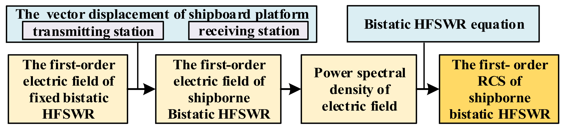
2.1. Derivation of a First-Order RCS of Shipborne Bistatic HFSWR

The general first-order scatter geometry of shipborne bistatic HFSWR is depicted in Figure 1. The electromagnetic wave from the transmitting station T, propagates along a path ${\overrightarrow{\rho }}_1$ and then follows a path, ${\overrightarrow{\rho }}_2$, to the receiving station R. ${\theta }_1$, ${\theta }_2$, ${\phi }_1$, and ${\phi }_2$ are the angles of the transmitting signal path (${\overrightarrow{\rho }}_1$), receiving signal path (${\overrightarrow{\rho }}_2$), transmitting antenna vector displacement ($\delta {\overrightarrow{\rho }}_1$), and receiving antenna vector displacement ($\delta {\overrightarrow{\rho }}_2$), respectively, measured anticlockwise with the baseline, $\overrightarrow{\rho }$, as the reference direction. As illustrated in Figure 1, when the ships that carry T and R, are moving, the new signal path lengths can be approximately estimated by:

$$\left|{\overrightarrow{\rho }}_1^{\prime }\right|=\sqrt{{\left({\overrightarrow{\rho }}_1-\delta {\overrightarrow{\rho }}_1\right)}^2}\cong \left|{\overrightarrow{\rho }}_1\right|\sqrt{1-2\frac{{\widehat{\rho }}_1·\delta {\overrightarrow{\rho }}_1}{{\rho }_1}}\cong {\rho }_1\sqrt{{(1-\frac{{\widehat{\rho }}_1·\delta {\overrightarrow{\rho }}_1}{{\rho }_1})}^2}={\rho }_1-{\widehat{\rho }}_1\delta {\overrightarrow{\rho }}_1$$

(1)

$$\left|{\overrightarrow{\rho }}_2^{\prime }\right|=\sqrt{{\left({\overrightarrow{\rho }}_2+\delta {\overrightarrow{\rho }}_2\right)}^2}\approx {\rho }_2+{\widehat{\rho }}_2\delta {\overrightarrow{\rho }}_2,$$

(2)

where ${\widehat{\rho }}_1$ and ${\widehat{\rho }}_2$ are the unit vectors of ${\overrightarrow{\rho }}_1$ and ${\overrightarrow{\rho }}_2$, respectively.

The derivation process of the first-order RCS equation for shipborne bistatic HFSWR is summarized in Figure 2. The derivation process is modified from that for fixed bistatic HFSWR presented in [9]. The process includes three steps, i.e., deriving the first-order electric field equation, calculating the autocorrelation function and power spectral density, and deducing the first-order RCS equation.

Step 1: The first-order scattering electric field

With reference to [9] and considering (1) and (2), the first-order scattered electric field of shipborne bistatic HFSWR can be modified as follows:

$$\begin{gathered} {\left(E_{0n}^{+}\right)}_1\approx \frac{k{C}_0}{{(2\pi )}^2}{{\displaystyle \sum }}_{\overrightarrow{K}}{P}_{\overrightarrow{K}}K\iint \cos ({\theta }_1-{\theta }_K)\frac{F\left({\rho }_1\right)F\left({\rho }_2\right)}{{\rho }_1{\rho }_2}· \\ {e}^{j{\rho }_{1}K\cos \left({\theta }_1-{\theta }_K\right)}{e}^{-jk\left({\rho }_1+{\rho }_2\right)}{e}^{-jk\left({\rho }_1+{\rho }_2-{\widehat{\rho }}_1\delta {\overrightarrow{\rho }}_1+{\widehat{\rho }}_2\delta {\overrightarrow{\rho }}_2\right)}d{x}_{1}d{y}_1, \end{gathered}$$

(3)

where $C_0$ equals $I{k}^2\Delta l/j\omega {ϵ}_0$, in which $I$ is the current on a dipole with length $\Delta l$, radian frequency $\omega$, and corresponding wavenumber $k=\omega /c$. The variables $c$ and ${ϵ}_0$ denote light speed and permittivity, respectively. $P_{\overrightarrow{K}}$ is the Fourier coefficient associated with a rough surface component with a wave vector of $\overrightarrow{K}$. Here, ${\theta }_K$ is the counterclockwise angle of $\overrightarrow{K}$ with reference to $\overrightarrow{\rho }$.

As shown in [9], for a bistatic HFSWR, it is more convenient to derive the electric field equation by converting the vectors from the $\mathrm{x}-\mathrm{y}$ Cartesian coordinate system into the ${\mu }_0-{\delta }_0$ elliptic coordinate system, where ${\mu }_0\in \left[0,+\infty \right]$, ${\delta }_0\in \left[0,2\pi \right]$. By applying a stationary phase method [9] to (3), a final electric field may be written as:

$${\left(E_{0n}^{+}\right)}_1\approx \frac{k{C}_0}{{(2\pi )}^{\frac{3}{2}}}{{\displaystyle \sum }}_{\overrightarrow{K}}{P}_{\overrightarrow{K}}\sqrt{Kcos\phi }{{\displaystyle \int }}_{\frac{\rho }{2}}^{\infty }\frac{F\left({\rho }_1\right)F\left({\rho }_2\right)}{\sqrt{{\rho }_s{}^2-{\left(\frac{\rho }{2}\right)}^2}}{e}^{j\overrightarrow{K}\frac{\overrightarrow{\rho }}{2}-j\frac{\pi }{4}+j{\rho }_{s}Kcos\phi -j2k{\rho }_s}{e}^{jk\left({\widehat{\rho }}_1\delta {\overrightarrow{\rho }}_1-{\widehat{\rho }}_2\delta {\overrightarrow{\rho }}_2\right)}d{\rho }_s,$$

(4)

where $\phi$ refers to the bistatic angle. The first-order electric field expression in the time domain can be expressed as:

$$\begin{gathered} {\left(E_{0n}^{+}\right)}_1\left(t\right)\approx \frac{-j{\eta }_0\Delta l{I}_0{k}_0{}^2}{{(2\pi )}^{\frac{3}{2}}}\frac{F\left({\rho }_1\right)F\left({\rho }_2\right)\Delta {\rho }_s}{\sqrt{{\rho }_s[{\rho }_s{}^2-{\left(\frac{\rho }{2}\right)}^2}]}{\displaystyle \sum }_{\overrightarrow{K}}{P}_{\overrightarrow{K}}\sqrt{Kcos\phi }Sa\left[\frac{\Delta {\rho }_s}{2}\left(\frac{K}{cos\phi }-2k_0\right)\right] \\ ·e^{j[\overrightarrow{K}\frac{\overrightarrow{\rho }}{2}-\frac{\pi }{4}+K{\rho }_{s}cos\phi +k_0\Delta {\rho }_s+\frac{K({\widehat{\rho }}_1\delta {\overrightarrow{\rho }}_1-{\widehat{\rho }}_2\delta {\overrightarrow{\rho }}_2)}{2cos\phi }+\omega t]}, \end{gathered}$$

(5)

where $t$ represents the time parameter; $I_0$ is the peak value of current $I$, which corresponds to wavenumber $k_0={\omega }_0/c$; and $\Delta {\rho }_s=c{\tau }_0/2$ is the scattering patch width that depends on the current pulse width, ${\tau }_0$. In addition, $Sa\left(x\right)=\frac{sinx}{x}$ represents the sampling function.

Step 2: Calculation of power spectral density of electric field

The autocorrelation function of electric field (5) in time domain is calculated by:

$$R\left(\tau \right)=\frac{A_r}{2{\eta }_0}{⟨\left(E_{0n}^{+}\right)}_1\left(t+\tau \right){\left(E_{0n}^{+}\right)}_1^{*}\left(t\right)⟩,$$

(6)

where $A_r=\left({\lambda }_0{}^2/4\pi \right)G_r$ is referred to as the effective free-space aperture of the receiving antenna; ${\lambda }_0$ is the free space wavelength of the transmitted signal; $G_r$ is the free-space gain of the receiving antenna; $\tau$ is the time gap between two consecutive measurements; and ${(·)}^{*}$ and $⟨·⟩$ are operations of complex conjugation and ensemble average, respectively.

By inserting (5) to (6), the autocorrelation of the time-domain electric field becomes

$$\begin{gathered} R\left(\tau \right)=\frac{{\lambda }_0{}^2{G}_r{\eta }_0\Delta l^2{I}_0{}^2{k}_0{}^4}{2^6{\pi }^4}·\frac{{\left|F\left({\rho }_1\right)F\left({\rho }_2\right)\right|}^2\Delta {\rho }_s{}^{2}cos\phi }{{\rho }_s[{\rho }_s{}^2-{\left(\rho /2\right)}^2]}\iiint K^{2}S\left(\overrightarrow{K},\omega \right) \\ ·S{a}^2\left[\frac{\Delta {\rho }_s}{2}\left(\frac{K}{cos\phi }-2k_0\right)\right]e^{j\omega \tau }⟨M\left(K,{\theta }_K,t,\tau \right)⟩d\tau d\omega dK d{\theta }_K, \end{gathered}$$

(7)

where the ocean wave spectrum, $S\left(\overrightarrow{K},\omega \right)$, is obtained from: $⟨{{\displaystyle \sum }}_{\overrightarrow{K_1}}{P}_{\overrightarrow{K_1}}·{{\displaystyle \sum }}_{\overrightarrow{K_2}}{P}_{\overrightarrow{K_2}}⟩=\left\{\begin{array}{c}{N}^2·W·S\left(\overrightarrow{K},\omega \right),\overrightarrow{K_1}=\overrightarrow{K_2}\\ 0,else\end{array}\right.$ [9].

$N^2$ is equivalent to $K·dK·d{\theta }_K$, and $W$ is equivalent to $d\omega$. $⟨M\left(K,{\theta }_K,t,\tau \right)⟩$ is a function of the displacement vector, and is expressed as:

$$M\left(K,{\theta }_K,t,\tau \right)=e^{\frac{jK}{2cos\phi }\left({\widehat{\rho }}_1\delta {\overrightarrow{\rho }}_1\left(t+\tau \right)-{\widehat{\rho }}_1\delta {\overrightarrow{\rho }}_1\left(t\right)\right)}·e^{\frac{jK}{2cos\phi }\left({\widehat{\rho }}_2\delta {\overrightarrow{\rho }}_2\left(t\right)-{\widehat{\rho }}_2\delta {\overrightarrow{\rho }}_2\left(t+\tau \right)\right)}$$

(8)

Applying Fourier transform to (7), i.e., $P\left({\omega }_d\right)=\mathcal{F}\left\{R\left(\tau \right)\right\}$, results in:

$$\begin{gathered} P\left({\omega }_d\right)=\frac{{\lambda }_0{}^2{G}_r{\eta }_0\Delta l^2{I}_0{}^2{k}_0{}^4}{2^6{\pi }^4}·\frac{{\left|F\left({\rho }_1\right)F\left({\rho }_2\right)\right|}^2\Delta {\rho }_s{}^{2}cos\phi }{{\rho }_s[{\rho }_s{}^2-{\left(\rho /2\right)}^2]}\iiint K^{2}S\left(\overrightarrow{K},\omega \right) \\ ·S{a}^2\left[\frac{\Delta {\rho }_s}{2}\left(\frac{K}{cos\phi }-2k_0\right)\right]\int e^{j\left(\omega -{\omega }_d\right)\tau }⟨M\left(K,{\theta }_K,t,\tau \right)⟩\mathrm{d}\tau d\omega dK d{\theta }_K \end{gathered}$$

(9)

Step 3: Calculation of the first-Order shipborne bistatic RCS

The power spectral density per unit area can be obtained by approximating scattering unit area as $dA\approx \frac{\Delta {\rho }_s{\left({\rho }_1{\rho }_2\right)}^2}{{\rho }_s[{\rho }_s{}^2-{\left(\rho /2\right)}^2]}d{\theta }_K$ [9], i.e.,

$$\begin{gathered} \frac{dP\left({\omega }_d\right)}{dA}=\frac{{\lambda }_0{}^2{G}_r{\eta }_0\Delta l^2{I}_0{}^2{k}_0{}^4}{2^6{\pi }^4}·\frac{{\left|F\left({\rho }_1\right)F\left({\rho }_2\right)\right|}^2\Delta {\rho }_{s}cos\phi }{{\left({\rho }_1{\rho }_2\right)}^2}\iint K^{2}S\left(\overrightarrow{K},\omega \right) \\ ·S{a}^2\left[\frac{\Delta {\rho }_s}{2}\left(\frac{K}{cos\phi }-2k_0\right)\right]\int e^{j\left(\omega -{\omega }_d\right)\tau }⟨M\left(K,{\theta }_K,t,\tau \right)⟩\mathrm{d}\tau d\omega dK \end{gathered}$$

(10)

By inserting (12) into (10) and comparing it with the bistatic radar range Equation (11), the first-order RCS Equation (13) can be derived. It should be noted that $g$ is gravity acceleration.

$$\frac{dP\left({\omega }_d\right)}{dA}=\frac{{\lambda }_0{}^2{G}_r{P}_t{G}_t{\left|F\left({\rho }_1\right)F\left({\rho }_2\right)\right|}^2}{{\left(4\pi \right)}^3{\left({\rho }_1{\rho }_2\right)}^2}\sigma \left({\omega }_d\right)$$

(11)

$$S\left(\overrightarrow{K},\omega \right)=\frac{1}{2}{\displaystyle \sum }_{m=\pm 1}S(m\overrightarrow{K})\delta ({\omega }_d+m\sqrt{gK})$$

(12)

$$\begin{gathered} \sigma \left({\omega }_d\right)=2^2{k}_0{}^2\Delta {\rho }_{s}cos\phi {\displaystyle \sum }_{m=\pm 1}\int K^{2}S(m\overrightarrow{K})S{a}^2\left[\frac{\Delta {\rho }_s}{2}\left(\frac{K}{cos\phi }-2k_0\right)\right] \\ ·{\displaystyle \int }{e}^{-j\left(m\sqrt{gK}+{\omega }_d\right)\tau }⟨M\left(K,{\theta }_K,t,\tau \right)⟩d\tau dK \end{gathered}$$

(13)

When $M\left(K,{\theta }_K,t,\tau \right)=0$, (13) is reduced to the first-order RCS for a stationary bistatic HFSWR. When $\delta {\overrightarrow{\rho }}_1$ and $\delta {\overrightarrow{\rho }}_2$ in $M\left(K,{\theta }_K,t,\tau \right)$ take 0 in turn, the first-order RCS can become the case where only the transmitter and receiver are moving.

2.2. First-Order RCS with Different Motion Types

The first-order RCS formulae for different types of motion are obtained. In this study, uniform linear, periodic oscillation, and hybrid motions are considered. It should be noted that both the transmitting and receiving platforms are assumed to undertake the same motion type.

2.2.1. First-Order RCS with Uniform Linear Motion

The displacement vectors in Equation (8) can be substituted by the uniform linear motion displacement vectors as given below:

$$\left\{\begin{array}{c}\delta {\overrightarrow{\rho }}_{1\mathrm{v}}\left(t\right)={\overrightarrow{v}}_{1}t\\ \delta {\overrightarrow{\rho }}_{2\mathrm{v}}\left(t\right)={\overrightarrow{v}}_{2}t\end{array}\right. ,$$

(14)

where ${\overrightarrow{v}}_1$ and ${\overrightarrow{v}}_2$ represent the uniform motion vectors of the transmitter and receiver, respectively, and ${\phi }_{1\mathrm{v}}$ and ${\phi }_{2\mathrm{v}}$ are substitutions of ${\phi }_1$ and ${\phi }_2$. Then, Equation (8) can be written as:

$$M_1=e^{\frac{jK\tau }{2cos\phi }\left[v_{1}cos\left({\phi }_{1\mathrm{v}}-{\theta }_1\right)-v_{2}cos\left({\phi }_{2\mathrm{v}}-{\theta }_2\right)\right]}$$

(15)

Because $M_1$ is independent of $t$, $⟨M_1⟩=M_1$. By substituting (15) into (13) and solving the integral about $\tau$, the first-order RCS for the case of uniform linear motion can be obtained as:

$$\begin{gathered} \sigma \left({\omega }_d\right)=2^3\pi k_0{}^2\Delta {\rho }_{s}cos\phi {\displaystyle \sum }_{m=\pm 1}\int K^{2}S(m\overrightarrow{K})S{a}^2\left[\frac{\Delta {\rho }_s}{2}\left(\frac{K}{cos\phi }-2k_0\right)\right] \\ ·\delta ({\omega }_d+m\sqrt{gK}-\frac{K}{2cos\phi }[v_{1}cos({\phi }_{1\mathrm{v}}-{\theta }_1)-v_{2}cos({\phi }_{2\mathrm{v}}-{\theta }_2)])dK \end{gathered}$$

(16)

${\theta }_1$ and ${\theta }_2$ are measured counterclockwise from the baseline reference direction, and they are both related to ${\theta }_K$.

$$\left\{\begin{array}{c}{\theta }_2={\theta }_K+\phi +\pi \\ {\theta }_1={\theta }_K-\phi \\ \phi =arcsin\left(esin{\theta }_K\right)\end{array}\right.,$$

(17)

where $e$ is the ellipse eccentricity of the detection area. Thus, (16) can be written in terms ${\theta }_K$ as:

$$\begin{gathered} \sigma \left({\omega }_d\right)=2^3\pi k_0{}^2\Delta {\rho }_{s}cos\phi {\displaystyle \sum }_{m=\pm 1}\int K^{2}S(m\overrightarrow{K})S{a}^2\left[\frac{\Delta {\rho }_s}{2}\left(\frac{K}{cos\phi }-2k_0\right)\right] \\ ·\delta \{{\omega }_d+m\sqrt{gK}-\frac{K{v}_1}{2}\left[cos\left({\phi }_{1\mathrm{v}}-{\theta }_K\right)-tan\phi sin\left({\phi }_{1\mathrm{v}}-{\theta }_K\right)\right] \\ -\frac{K{v}_2}{2}\left[cos\left({\phi }_{2\mathrm{v}}-{\theta }_K\right)+tan\phi sin\left({\phi }_{2\mathrm{v}}-{\theta }_K\right)\right]\}dK \end{gathered}$$

(18)

When $\Delta {\rho }_s\to \infty$, $\Delta {\rho }_{s}S{a}^2\left[\frac{\Delta {\rho }_s}{2}\left(\frac{K}{cos\phi }-2k_0\right)\right]=2\pi cos\phi \delta \left(K-2k_{0}cos\phi \right)$, the integral about $K$ in (18) can be solved. As a result, (18) is simplified as:

$$\begin{gathered} \sigma \left({\omega }_d\right)=2^6{\pi }^2{k}_0{}^{4}co{s}^4\phi {\displaystyle \sum }_{m=\pm 1}S(m\overrightarrow{K}) \\ ·\delta \{{\omega }_d+m\sqrt{2g{k}_0}-k_0{v}_1\left[cos\left({\phi }_{1\mathrm{v}}-{\theta }_K\right)-tan\phi sin\left({\phi }_{1\mathrm{v}}-{\theta }_K\right)\right] \\ -k_0{v}_2\left[cos\left({\phi }_{2\mathrm{v}}-{\theta }_K\right)+tan\phi sin\left({\phi }_{2\mathrm{v}}-{\theta }_K\right)\right]\} \end{gathered}$$

(19)

Next, the following two special cases are considered:

When the transmitter and receiver are sailing with the same speed and direction (i.e., $v_1=v_2=v$; ${\phi }_{1\mathrm{v}}={\phi }_{2\mathrm{v}}={\phi }_{\mathrm{v}}$), (19) becomes:

$$\sigma \left({\omega }_d\right)=2^6{\pi }^2{k}_0{}^{4}co{s}^4\phi {\displaystyle \sum }_{m=\pm 1}S(m\overrightarrow{K})\delta \left[{\omega }_d+m\sqrt{2g{k}_0}-2k_{0}vcos\left({\phi }_{\mathrm{v}}-{\theta }_K\right)\right]$$

(20)

For a relatively far detection range or other specific conditions that make the bistatic angle, $\phi$, approach 0, (20) is further simplified as:

$$\sigma \left({\omega }_d\right)=2^6{\pi }^2{k}_0{}^4{{\displaystyle \sum }}_{m=\pm 1}S(m\overrightarrow{K})\delta \left[{\omega }_d+m\sqrt{2g{k}_0}-2k_{0}vcos\left({\phi }_{\mathrm{v}}-{\theta }_K\right)\right]$$

(21)

Equation (21) is consistent with the formula given by Xie in [12]. Therefore, the shipborne bistatic first-order RCS in this case is equivalent to the shipborne monostatic result.

When the transmitter and receiver are sailing at same speed but in opposite directions (i.e., $v_1=v_2=v$; ${\phi }_{1\mathrm{v}}={\phi }_{2\mathrm{v}}+\pi ={\phi }_{\mathrm{v}}$), (19) becomes:

$$\sigma \left({\omega }_d\right)=2^6{\pi }^2{k}_0{}^{4}co{s}^4\phi {\displaystyle \sum }_{m=\pm 1}S(m\overrightarrow{K})\delta \left[{\omega }_d+m\sqrt{2g{k}_0}+2k_{0}vtan\phi sin\left({\phi }_{\mathrm{v}}-{\theta }_K\right)\right]$$

(22)

Similarly, if the bistatic angle, $\phi$, approaches 0, (22) can be simplified as:

$$\sigma \left({\omega }_d\right)=2^6{\pi }^2{k}_0{}^4{\displaystyle \sum }_{m=\pm 1}S(m\overrightarrow{K})\delta \left({\omega }_d+m\sqrt{2g{k}_0}\right)$$

(23)

Interestingly, it can be seen that in the case of a long detection range and a small bistatic angle, the first-order RCS is independent of the platform’s speed, so its characteristics are similar to those of the shore-based case.

2.2.2. First-Order RCS with Periodic Oscillation Motion

The transmitter and receiver of bistatic shipborne radar are also subject to the effect of ocean waves, which cause periodic oscillation motion. The displacement vectors in (8) can be expressed as vectors for periodic motion displacement as:

$$\left\{\begin{array}{c}\delta {\overrightarrow{\rho }}_{1\mathrm{s}}\left(t\right)={\widehat{\rho }}_{1s}{\mathsf{\alpha }}_{1s}sin\left({\omega }_{1s}t\right)\\ \delta {\overrightarrow{\rho }}_{2\mathrm{s}}\left(t\right)={\widehat{\rho }}_{2s}{\mathsf{\alpha }}_{2s}sin\left({\omega }_{2s}t\right)\end{array}\right.$$

(24)

where ${\widehat{\rho }}_{1s}$ and ${\widehat{\rho }}_{2s}$ represent the unit vectors in the direction of oscillation motion for the transmitter and receiver, respectively; ${\mathsf{\alpha }}_{1s}$, ${\mathsf{\alpha }}_{2s}$, and ${\omega }_{1s}$, ${\omega }_{2s}$ are the amplitudes and ocean-wave frequencies of their oscillation motions, respectively. According to the description of a ship’s motion due to waves [23], when ${\widehat{\rho }}_{1s}$ is perpendicular to the hull of the transmitting platform, the periodic motion can be regarded as sway. If ${\widehat{\rho }}_{1s}$ is parallel to the hull of the transmitting station, the periodic oscillation motion can be treated as surge. The same applies to ${\widehat{\rho }}_{2s}$. For better denotation, angles ${\phi }_1$ and ${\phi }_2$ are replaced by ${\phi }_{1\mathrm{s}}$ and ${\phi }_{2\mathrm{s}}$.

In this case, $M_2$ in (8) can be simplified as:

$$\begin{gathered} M_2=e^{\frac{jK}{2cos\phi }\left\{2{\mathsf{\alpha }}_{1s}cos\left({\phi }_{1\mathrm{s}}-{\theta }_1\right)\left[sin\left(\frac{1}{2}{\omega }_{1s}\tau \right)cos\left({\omega }_{1s}t+\frac{1}{2}{\omega }_{1s}\tau \right)\right]\right\}} \\ \hspace{1em}\hspace{1em} ·e^{\frac{-jK}{2cos\phi }\left\{2{\mathsf{\alpha }}_{2s}cos\left({\phi }_{2\mathrm{s}}-{\theta }_2\right)\left[sin\left(\frac{1}{2}{\omega }_{2s}\tau \right)cos\left({\omega }_{2s}t+\frac{1}{2}{\omega }_{2s}\tau \right)\right]\right\}} \end{gathered}$$

(25)

It can be written as a Bessel function as:

$$⟨M_2⟩={\mathrm{J}}_0(2{\mathrm{x}}_{1}sin(\frac{{\Phi }_1}{2})){\mathrm{J}}_0(2{\mathrm{x}}_{2}sin(\frac{{\Phi }_2}{2})),$$

(26)

where ${\mathrm{J}}_0$ is a zero-order Bessel function, and ${\mathrm{x}}_1$ and ${\mathrm{x}}_2$ are:

$$\left\{\begin{array}{c}{\mathrm{x}}_1=\frac{{\mathsf{\alpha }}_{1s}K}{2cos\phi }cos\left({\phi }_{1\mathrm{s}}-{\theta }_1\right); {\Phi }_1={\omega }_{1s}\tau \\ {\mathrm{x}}_2=\frac{{\mathsf{\alpha }}_{2s}K}{2cos\phi }cos\left({\phi }_{2\mathrm{s}}-{\theta }_2\right); {\Phi }_2={\omega }_{2s}\tau \end{array}\right.$$

(27)

According to the properties of the Bessel function [11]:

$${\mathrm{J}}_0(2xsin\frac{\Phi }{2})={\mathrm{J}}_0{}^2(x)+2{\displaystyle \sum }_{n=1}^{+\infty }{\mathrm{J}}_n{}^2(x)cos(n\Phi )$$

(28)

Equation (26) can be found to be:

$$\begin{gathered} ⟨M_2⟩={\mathrm{J}}_0{}^2\left(x_1\right){\mathrm{J}}_0{}^2\left(x_2\right)+{\displaystyle \sum }_{m_1=1}^{+\infty }{\mathrm{J}}_0{}^2\left(x_1\right){\mathrm{J}}_{m_1}{}^2\left(x_2\right)\left(e^{j{m}_1{\omega }_{2s}\tau }+e^{-j{m}_1{\omega }_{2s}\tau }\right) \\ +{\displaystyle \sum }_{m_2=1}^{+\infty }{\mathrm{J}}_0{}^2\left(x_2\right){\mathrm{J}}_{m_2}{}^2\left(x_1\right)\left(e^{j{m}_2{\omega }_{1s}\tau }+e^{-j{m}_2{\omega }_{1s}\tau }\right)+{\displaystyle \sum }_{n_1=1}^{+\infty }{\displaystyle \sum }_{n_2=1}^{+\infty }{\mathrm{J}}_{n_1}{}^2\left(x_2\right){\mathrm{J}}_{n_2}{}^2\left(x_1\right) \\ ·[e^{j(n_1{\omega }_{1s}+n_2{\omega }_{2s})\tau }+e^{-j(n_1{\omega }_{1s}+n_2{\omega }_{2s})\tau }+e^{j(n_1{\omega }_{1s}-n_2{\omega }_{2s})\tau }+e^{j(-n_1{\omega }_{1s}+n_2{\omega }_{2s})\tau }] \end{gathered}$$

(29)

By substituting (29) into (13), then solving the integral of $\tau$, the first-order RCS of bistatic shipborne HFSWR with periodic oscillation motion can be obtained as:

$$\begin{gathered} \sigma \left({\omega }_d\right)=2^3\pi k_0{}^2\Delta {\rho }_{s}cos\phi {\displaystyle \sum }_{m=\pm 1}\int K^{2}S(m\overrightarrow{K})S{a}^2\left[\frac{\Delta {\rho }_s}{2}\left(\frac{K}{cos\phi }-2k_0\right)\right]\hspace{1em}\hspace{1em}\hspace{1em}\hspace{1em}\hspace{1em}\hspace{1em}\hspace{1em}\hspace{1em} \\ ·\{{\displaystyle \sum }_{n_1=0}^{+\infty }{\displaystyle \sum }_{n_2=0}^{+\infty }{\displaystyle \sum }_{m_1=\pm 1}{\displaystyle \sum }_{m_2=\pm 1}{\mathrm{J}}_{n_1}{}^2\left[\frac{{\mathsf{\alpha }}_{1s}K}{2cos\phi }cos\left({\phi }_{1\mathrm{s}}-{\theta }_1\right)\right] \\ ·{\mathrm{J}}_{n_2}{}^2\left[\frac{{\mathsf{\alpha }}_{2s}K}{2cos\phi }cos\left({\phi }_{2\mathrm{s}}-{\theta }_2\right)\right]\delta \left({\omega }_d+m\sqrt{gK}+m_1{n}_1{\omega }_{1s}+m_2{n}_2{\omega }_{2s}\right)\}dK \end{gathered}$$

(30)

Equation (30) contains an infinite number of Bessel functions. However, the effects of the third-order and higher-order Bessel functions can be ignored. It can be observed that the periodic oscillation motion of the platforms results in additional peaks in the first-order RCS. Next, the formula for each peak is analyzed.

In the case of $n_1=0, 1, 2$, $n_2=0, 1, 2$ they correspond to eight peaks:

$$\begin{gathered} {\sigma }_{n_1{n}_{2}1}\left({\omega }_d\right)=2^4\pi k_0{}^2\Delta {\rho }_{s}cos\phi \frac{\sqrt{K}{K}^2}{\sqrt{g}}S{a}^2\left[\frac{\Delta {\rho }_s}{2}\left(\frac{K}{cos\phi }-2k_0\right)\right] \\ ·J_{n_1}{}^2\left[\frac{{\alpha }_{1s}K}{2cos\phi }cos\left({\phi }_{1s}-{\theta }_1\right)\right]J_{n_2}{}^2\left[\frac{{\alpha }_{2s}K}{2cos\phi }cos\left({\phi }_{2s}-{\theta }_2\right)\right] \\ ·\mathrm{S}(\mathrm{sgn}\left(-{\mathsf{\omega }}_{\mathrm{d}}\pm {\mathrm{n}}_1{\mathsf{\omega }}_{1\mathrm{s}}\pm {\mathrm{n}}_2{\mathsf{\omega }}_{2\mathrm{s}}\right)\overrightarrow{\mathrm{K}}), \end{gathered}$$

(31)

where $K={\left({\omega }_d\mp n_1{\omega }_{1s}\mp n_2{\omega }_{2s}\right)}^2/g$. (31) is derived by applying $dK=\frac{2\sqrt{K}}{\sqrt{g}}d{\omega }_d$ to the integral of $K$. When $K=2k_{0}cos\phi$, ${\sigma }_{00}$ reaches its maximum.

When ${\omega }_{1s}={\omega }_{2s}={\omega }_s$, (31) can be written as:

$$\begin{gathered} {\sigma }_{n_1{n}_{2}1}\left({\omega }_d\right)=2^4\pi k_0{}^2\Delta {\rho }_{s}cos\phi \frac{\sqrt{K}{K}^2}{\sqrt{g}}S{a}^2\left[\frac{\Delta {\rho }_s}{2}\left(\frac{K}{cos\phi }-2k_0\right)\right] \\ ·J_{n_1}{}^2\left[\frac{{\alpha }_{1s}K}{2cos\phi }cos\left({\phi }_{1s}-{\theta }_1\right)\right]J_{n_2}{}^2\left[\frac{{\alpha }_{2s}K}{2cos\phi }cos\left({\phi }_{2s}-{\theta }_2\right)\right] \\ ·\mathrm{S}(\mathrm{sgn}\left(-{\mathsf{\omega }}_{\mathrm{d}}+\left(\pm {\mathrm{n}}_1\pm {\mathrm{n}}_2\right){\mathsf{\omega }}_{\mathrm{s}}\right)\overrightarrow{\mathrm{K}}) \end{gathered}$$

(32)

In the case of (32), the number of additional peaks decreases.

2.2.3. First-Order RCS with Hybrid Motion

In this case, the transmitter and receiver undertake both uniform linear motion and periodic oscillation motion. (8) can be replaced by combining (15) and (26). Finally, the first-order RCS of bistatic shipborne HFSWR with uniform linear and periodic oscillation motion can be obtained as:

$$\begin{array}{l}\sigma \left({\omega }_d\right)=2^3\pi k_0{}^2\Delta {\rho }_{s}cos\phi {\displaystyle \sum }_{m=\pm 1}\int K^{2}S\left(m\overrightarrow{K}\right)S{a}^2\left[\frac{\Delta {\rho }_s}{2}\left(\frac{K}{cos\phi }-2k_0\right)\right]\\ ·\{{\displaystyle \sum }_{n_1=0}^{+\infty }{\displaystyle \sum }_{n_2=0}^{+\infty }{\displaystyle \sum }_{m_1=\pm 1}{\displaystyle \sum }_{m_2=\pm 1}{\mathrm{J}}_{n_1}{}^2\left[\frac{{\mathsf{\alpha }}_{1s}K}{2cos\phi }cos\left({\phi }_{1\mathrm{s}}-{\theta }_1\right)\right]{\mathrm{J}}_{n_2}{}^2\left[\frac{{\mathsf{\alpha }}_{2s}K}{2cos\phi }cos\left({\phi }_{2\mathrm{s}}-{\theta }_2\right)\right]\\ ·\delta ({\omega }_d+m\sqrt{gK}-\frac{K}{2cos\phi }\left[v_{1}cos\left({\phi }_{1\mathrm{v}}-{\theta }_1\right)-v_{2}cos\left({\phi }_{2\mathrm{v}}-{\theta }_2\right)\right]\\ +m_1{n}_1{\omega }_{1s}+m_2{n}_2{\omega }_{2s})\}dK\end{array}$$

(33)

When the angle difference between ${\phi }_{1\mathrm{s}}$ and ${\phi }_{1\mathrm{v}}$ is $90°$, the oscillation motion of the transmitter is the sway. When ${\phi }_{1\mathrm{s}}$ and ${\phi }_{1\mathrm{v}}$ are equal, the oscillation motion of the transmitting platform is the surge. Similarly, the relationship between ${\phi }_{2\mathrm{s}}$ and ${\phi }_{2\mathrm{v}}$ determines the type of oscillation of the receiving platform.

3. Simulation Results and Discussion

Based on the derived RCS models, the first-order Doppler spectra from the ocean surface under the aforementioned three types of motion states are simulated to investigate corresponding characteristics. The parameters for the simulation are as follows: the radar frequency is 4.7 MHz, the length of the baseline (distance between the receiving platform to transmitting platform) is 10 km, the baseline direction (from the transmitting platform to the receiving platform) is 0°, and the counterclockwise direction is positive. As in most previous research, the Pierson–Moskowitz spectrum [24] is used in the simulation, and the wind speed is selected as 12 m/s. The wind direction is 60° for the simulations in Figure 3 and Figure 4, and the others are 0°. Additionally, the ocean current effect is ignored.

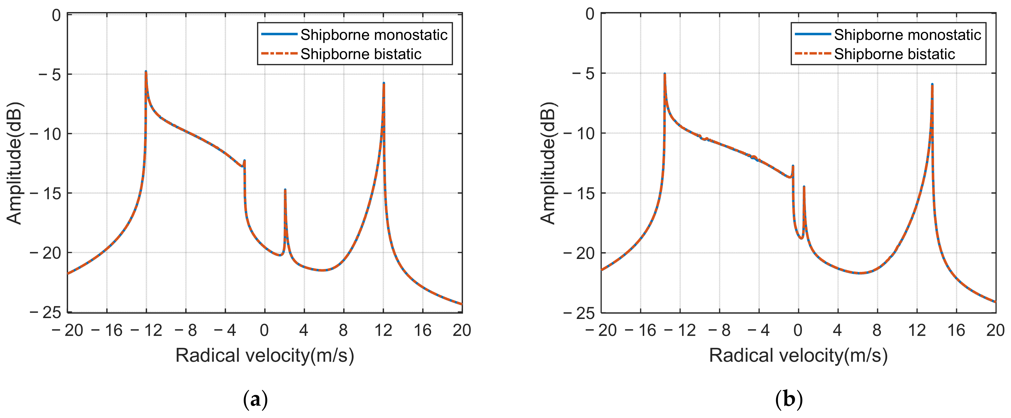
3.1. Both Platforms Move in Uniform Linear Motion

Figure 3 shows the first-order Doppler spectra for the case when the transmitting and receiving platforms are moving in same direction and at the same speed with a total signal propagation range of 150 km. In Figure 3a,b, the platforms’ moving velocities are 5 m/s and 6.5 m/s, respectively, and the moving direction is 180°. For comparison, the RCS simulation results (blue solid line) for shipborne monostatic radar under the same motion direction and speed are also given in Figure 3. According to (21) and Figure 3, when the detection range of shipborne bistatic HFSWR is far, the shipborne bistatic HFSWR first-order RCS is similar to that of a shipborne monostatic HFSWR.

In Figure 4a,b, the first-order peaks are spread when the transmitter and receiver platforms move at the same speed and in the same direction along the baseline. Its spread width is consistent with the results of shipborne monostatic HFSWR. According to the comparison of Figure 3a,b, increased platform speed causes a larger spread width in the first-order spectrum, and this property is the same as that of shipborne monostatic radar.

Similarly, Figure 4 shows the first-order Doppler spectrum for the case in which all the settings are the same as those in Figure 3, except the range sum is 50 km. In Figure 4a,b, the first-order Doppler spectra amplitude of shipborne bistatic HFSWR is slightly different from that of shipborne monostatic HFSWR. This difference is due to the change in bistatic angle, and it is almost negligible.

According to Figure 3 and Figure 4, it can be concluded that the shipborne bistatic first-order Doppler spectrum can be approximately equivalent to that of the shipborne monostatic system when the transmitting and receiving platforms of the former are moving in same direction and at same speed along the baseline.

Figure 5 shows the shipborne bistatic first-order Doppler spectrum when the transmitting and receiving platforms move in opposite directions (0° and 180°) but at the same speed. The detection range sum is 150 km. The shore-based bistatic first-order Doppler spectra are also displayed with a blue solid line. In Figure 5a,b, the motion velocities are 5 m/s and 10 m/s, respectively.

It can be seen from Figure 5a that the shipborne bistatic first-order Doppler spectra are similar to those of shore-based bistatic radar. Few spreads are seen because the spread width is much smaller than that in the case with platforms moving in the same direction, as shown in Figure 3a. From comparison between Figure 5a,b, increasing the platform speed from 5 m/s to 10 m/s only slightly increases the spread width of the shipborne bistatic first-order peaks by about 0.34 m/s. However, if the platform speed of the shipborne monostatic HFSWR is increased from 5 m/s to 10 m/s under the same conditions, its first-order peak spread width is increased by 10 m/s. Furthermore, in the case of long-range detection, when the transmitting and receiving platforms move in opposite directions at same speed along the baseline, the shipborne bistatic first-order Doppler spectrum is similar to that of shore-based bistatic HFSWR.

In Figure 5, both platforms are moving along the baseline. Next, the detection range sum is maintained as 150 km, and the receiving platform moving speed and direction are 10 m/s and 185°, respectively. Figure 6 shows another configuration where the two shipborne platforms do not move along the baseline. In Figure 6a, the direction of the transmitting platform is −2.4°. The motion speeds of the transmitting platform are 10 m/s and 8 m/s, respectively, and the corresponding first-order RCSs are represented by the red dotted line and blue solid line, respectively. In Figure 6b, the speed of the transmitting platform is 10 m/s. The motion directions of the transmitting platform are −2.4° and 12.6°, respectively, and the corresponding first-order RCSs are represented by the red dotted line and blue solid line, respectively.

It can be seen from Figure 6a,b that the first-order Doppler spectrum for a motion speed of 10 m/s and direction of −2.4° has a much smaller spread width. This result implies that when the motion configuration of the receiving platform is fixed, it is feasible to adjust the transmitting platform motion to reduce the spread of the first-order peaks. With optimal configuration, the first-order spectrum becomes similar to that of shore-based bistatic HFSWR (see Figure 5b). It also indicates that the transmitting and receiving platforms moving in opposite directions but at the same speed along the baseline is a non-optimal configuration and should be avoided. On the premise of fixing the receiving platform’s moving direction and speed, it is necessary to adjust the transmitting platform moving direction and speed to achieve an optimal configuration. In the case of the optimal configuration, the first-order peaks are much less spread; thus, the target signals may not be covered by the first-order spectrum so that the target detection performance of HFSWR can be improved.

Figure 7 shows the shipborne bistatic first-order Doppler spectrum results under two different motion configurations. Both configurations are for a detection distance of 50 km and a platform speed of 10 m/s. One configuration is for platforms moving in the opposite direction along the baseline, and the other is for non-baseline motion. In the former, the moving directions of the transmitting and receiving platforms are 0° and 180°, respectively, but they are 12° and 192°, respectively, in the latter. In addition, the variation of the first-order spectrum spread width with detection distance for the two cases is illustrated in Figure 7b, in which red and blue colors represent non-baseline and baseline cases, respectively.

It can be seen from Figure 7a, that the baseline motion case has a larger spread width, whereas the non-baseline motion shows a smaller spread width. At the short detection range, the spread width of the first-order peaks for the baseline motion with opposite directions is large. In addition, according to the spread range shown in Figure 7b, the spread width of the non-baseline motion is not wider than that of the baseline motion for farther detection distance, although a smaller widening occurs in closer range cells. The results indicate that the first-order peak spread width is not only dependent on the motion configuration of the transmitting and receiving platforms but is also affected by the detection distance.

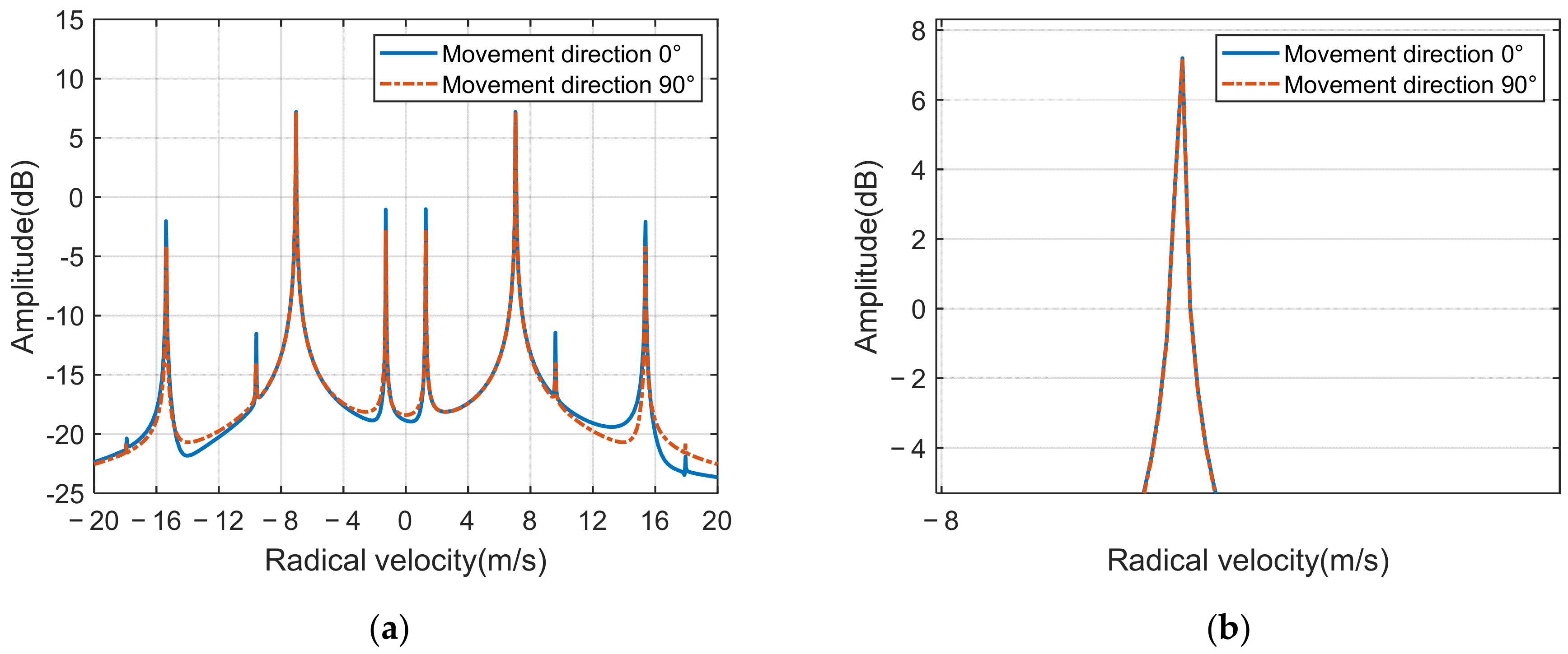
3.2. Both Platforms Move in Periodic Oscillation Motion

Figure 8 displays the simulated first-order Doppler spectra of the shipborne bistatic HFSWR with the transmitting and receiving platforms undertaking periodic oscillation motion at the same time. It is assumed that the transmitting and receiving platforms are located in two sea areas with different periodic oscillation motions. The oscillation amplitude and frequency of the transmitting platform are 0.177 and 0.261, respectively, and those of the receiving platform are 0.581 and 0.174, respectively. The direction of oscillation motion is 0°, and the detection range sum is 100 km. The first-order Doppler spectrum of shore-based bistatic HFSWR without oscillation motion (red dotted lines) is also shown for comparison.

It can be seen from Figure 8a that when the transmitting and receiving platforms have different oscillations, many motion-induced peaks appear in the shipborne bistatic first-order Doppler spectrum. These motion-induced peaks are not uniformly distributed on the Doppler frequency axis, and their locations depend on the oscillating motion frequencies. This phenomenon is caused by the oscillation property of the Bessel function. In Figure 8b, eight motion-induced peaks appear on one side of the positive Bragg peak in the first-order Doppler spectrum, and they significantly affect the target detection performance of shipborne bistatic HFSWR.

When the distance between the transmitting platform and the receiving platform is not large, the frequency and amplitude of the oscillation motion of the platform caused by the ocean waves are similar. Figure 9 displays shipborne bistatic first-order Doppler spectra when the transmitting and receiving platforms undertake the same oscillation motions (the oscillation amplitude is 0.177 and the frequency is 0.261). In Figure 9, the blue solid line is the first-order Doppler spectrum with a platform oscillation direction of 0°, and the red dotted line is for an oscillation direction of 90°.

It can be seen from Figure 9a that the first-order Doppler spectrum has fewer motion-induced peaks because motion-induced peaks caused by the transmitter and receiver motions overlap due to the same oscillation frequency values. Through comparison of the first-order RCS obtained under the two oscillation conditions, it can be observed that the amplitudes of the additional peaks depend on the oscillation direction. However, it can be seen from Figure 9b that the change in the direction of the oscillation motion does not affect the Bragg peak.

3.3. Both Platforms Undertake Periodic Motion and Uniform Linear Motion

Figure 10 shows the first-order Doppler spectra when the transmitting and receiving platforms undertake uniform linear motion and periodic oscillation motion at the same time. The transmitting and receiving platforms move at same speed (10 m/s) and in opposite directions (0°, 180°), but their oscillating motion directions, amplitudes (0.177), and frequencies (0.261) are equal. In Figure 10, the blue solid line represents the first-order Doppler spectrum with a platform oscillation direction of 0°, and the red dotted line is 90°.

It can be seen from Figure 10 that in the case of hybrid motion, motion-induced peaks are spread, and their widths are comparable to the spread width of the Bragg peak. A comparison of the results with two different oscillation directions shows that the spread widths of these additional peaks change little, although the amplitudes change considerably. In addition, the Bragg peak is not affected by the change of oscillation direction.

4. Conclusions

In this paper, first-order shipborne bistatic HFSWR RCS models for the cases of uniform linear, periodic oscillation, and hybrid platform motions are derived and simulated. The simulation results show that the difference in the moving directions of the transmitting and receiving platforms in a uniform linear motion lead to a considerable difference in the first-order spectrum. When the transmitting and receiving platforms move in the same direction and at the same speed along the baseline, the shipborne bistatic first-order spectrum of spreads. The spread width increases with the speed of the platforms, and the first-order RCS result is similar to that of shipborne monostatic HFSWR. When the shipborne bistatic platforms move in opposite directions along the baseline, the spread width of the first-order spectrum is small and is less sensitive to the platforms’ speed at a long detection range; thus, this case is equivalent to a shore-based bistatic HFSWR. In addition, when the transmitting and receiving platforms are both in periodic oscillation motions, fewer motion-induced peaks appear in the first-order spectrum if the oscillation motion parameters of the two platforms are same. For the shipborne bistatic configuration with platforms moving in opposite directions but at the same speed along the baseline, the broadening and amplitude of the Bragg peaks are not affected if the two platforms do not change and undertake the same oscillation motions. The direction of oscillation motion only affects the amplitudes of the motion-induced peaks. These conclusions are useful for selecting optimal motion configuration of shipborne platforms for shipborne bistatic HFSWR to be employed in marine target monitoring.

It should be noted that the above analysis assumes the simulation results of the two shipborne platforms under the same motion types and focuses on the first-order spectrum-broadening characteristics of shipborne bistatic HFSWR. The motion states of two shipborne platforms could be very complex and can be combined in many ways. How to optimize the motion parameters of the two platforms to minimize the broadening of the first-order echo spectrum will continue to be studied in the future. It is also necessary to validate the results using experimental data once they are available.

References

1. Barrick, D.E. Remote sensing of sea state by radar. In Proceedings of the Ocean 72nd IEEE International Conference on Engineering in the Ocean Environment, Newport, RI, USA, 13–15 September 1972; pp. 186–192. [Google Scholar]
2. Lipa, B.J.; Barrick, D.E. Extraction of sea state from HF radar sea echo: Mathematical theory and modeling. Radio Sci. 1986, 21, 81–100. [Google Scholar] [CrossRef]
3. Grosdidier, S.; Baussard, A.; Khenchaf, A. HFSW Radar Model: Simulation and Measurement. IEEE Trans. Geosci. Remote Sens. 2010, 48, 3539–3549. [Google Scholar] [CrossRef]
4. Xie, J.; Yao, G.; Sun, M.; Ji, Z. Measuring Ocean Surface Wind Field Using Shipborne High-Frequency Surface Wave Radar. IEEE Trans. Geosci. Remote Sens. 2018, 56, 3383–3397. [Google Scholar] [CrossRef]
5. Yao, G.; Xie, J.; Huang, W.; Ji, Z.; Zhou, W. Theoretical analysis of the first-order sea clutter in shipborne high-frequency surface wave radar. In Proceedings of the 2018 IEEE Radar Conference, Oklahoma City, OK, USA, 23–27 April 2018; pp. 1255–1259. [Google Scholar]
6. Sun, M.; Xie, J.; Ji, Z.; Cai, W. Remote sensing of ocean surface wind direction with shipborne high frequency surface wave radar. In Proceedings of the 2015 IEEE Radar Conference, Johannesburg, South Africa, 27–30 October 2015; pp. 39–44. [Google Scholar]
7. Liu, C.; Chen, B.; Chen, D.; Zhang, S. Analysis of First-order Sea Clutter in a Shipborne Bistatic High Frequency Surface Wave Radar. In Proceedings of the 2006 CIE International Conference on Radar, Shanghai, China, 16–19 October 2006; pp. 1–4. [Google Scholar]
8. Barrick, D.E. First-order theory and analysis of MF/HF/VHF scatter from the sea. IEEE Trans. Antennas Propag. 1972, 20, 2–10. [Google Scholar] [CrossRef] [Green Version]
9. Gill, E.W.; Walsh, J. High-frequency bistatic cross sections of the ocean surface. Radio Sci. 2001, 36, 1459–1475. [Google Scholar] [CrossRef]
10. Gill, E.W.; Huang, W.; Walsh, J. The Effect of the Bistatic Scattering Angle on the High-Frequency Radar Cross Sections of the Ocean Surface. IEEE Geosci. Remote Sens. Lett. 2008, 5, 143–146. [Google Scholar] [CrossRef]
11. Walsh, J.; Huang, W.; Gill, E.W. The First-Order High Frequency Radar Ocean Surface Cross Section for an Antenna on a Floating Platform. IEEE Trans. Antennas Propag. 2010, 58, 2994–3003. [Google Scholar] [CrossRef]
12. Xie, J.; Sun, M.; Ji, Z. First-order Ocean surface cross-section for shipborne HFSWR. Electron. Lett. 2013, 49, 1025–1026. [Google Scholar] [CrossRef]
13. Yao, G.; Xie, J.; Ji, Z.; Sun, M. The first-order ocean surface cross section for shipborne HFSWR with rotation motion. In Proceedings of the 2017 IEEE Radar Conference, Seattle, WA, USA, 8–12 May 2017; pp. 0447–0450. [Google Scholar]
14. Ma, Y.; Gill, E.W.; Huang, W. First-order high frequency radar ocean surface cross section incorporating a dual-frequency platform motion model. In Proceedings of the OCEANS 2016 MTS/IEEE Monterey, Shanghai, China, 10–13 April 2016; pp. 1–4. [Google Scholar]
15. Sun, M.; Xie, J.; Ji, Z.; Yao, G. Ocean surface cross sections for shipborne HFSWR with sway motion. Radio Sci. 2016, 51, 1745–1757. [Google Scholar] [CrossRef] [Green Version]
16. Ma, Y.; Gill, E.W.; Huang, W. Bistatic High-Frequency Radar Ocean Surface Cross Section Incorporating a Dual-Frequency Platform Motion Model. IEEE J. Ocean. Eng. 2018, 43, 205–210. [Google Scholar] [CrossRef]
17. Ma, Y.; Huang, W.; Gill, E.W. High-Frequency Radar Ocean Surface Cross Section Incorporating a Dual-Frequency Platform Motion Model. IEEE J. Ocean. Eng. 2018, 43, 195–204. [Google Scholar] [CrossRef]
18. Yao, G.; Xie, J.; Huang, W. Ocean Surface Cross Section for Bistatic HF Radar Incorporating a Six DOF Oscillation Motion Model. Remote Sens. 2019, 10, 2738. [Google Scholar] [CrossRef] [Green Version]
19. Zhu, Y.; Wei, Y.; Tong, P. First order sea clutter cross section for bistatic shipborne HFSWR. J. Syst. Eng. Electron. 2017, 28, 681–689. [Google Scholar]
20. Ji, Y.; Zhang, J.; Wang, Y. Coast–Ship Bistatic HF Surface Wave Radar: Simulation Analysis and Experimental Verification. Remote Sens. 2020, 12, 470. [Google Scholar] [CrossRef] [Green Version]
21. Ji, Z.; Jiang, X.; Xie, J.; Wang, Y.; Ding, J. Influence of bistatic shipborne HFSWOTHR platform oscillation on the sea clutter. In Proceedings of the International Conference on Signal Processing, Gold Coast, Australia, 15–17 December 2014; pp. 2007–2012. [Google Scholar]
22. Liu, J.; Ji, Y.; Liu, Y.; Meng, J.; Wang, Y.; Zhang, H. Simulation analysis of first order sea clutter spectrum for shipborne bistatic HFSWR. In Proceedings of the IET International Radar Conference, Chongqing, China, 4–6 November 2020; pp. 1656–1660. [Google Scholar]
23. Das, S.N.; Shiraishi, S.; Das, S.K. Mathematical modeling of sway, roll and yaw motions: Order-wise analysis to determine coupled characteristics and numerical simulation for restoring moment’s sensitivity analysis. Acta Mech. 2010, 213, 305–322. [Google Scholar] [CrossRef]
24. Pierson, W.J.; Moskowiz, L. A proposed spectral form for fully developed seas based upon the similarity theory of S. A. Kitaigorodskii. J. Geophys. Res. 1964, 69, 5181–5190. [Google Scholar] [CrossRef]
Figure 1. First-order bistatic shipborne HFSWR scatter geometry.
Jmse 10 00649 g001
Figure 2. Derivation process of the first order RCS.
Jmse 10 00649 g002
Figure 3. Simulated shipborne bistatic (red dotted line) and shipborne monostatic (blue solid line) first-order Doppler spectra for a detection range sum of 150 km. (a) The platforms’ speed is 5 m/s. (b) The platforms’ speed is 6.5 m/s.
Jmse 10 00649 g003
Figure 4. Simulated shipborne bistatic (red dotted line) and shipborne monostatic (blue solid line) first-order Doppler spectra for a detection range sum of 50 km. (a) The platforms’ speed is 5 m/s. (b) The platforms’ speed is 6.5 m/s.
Jmse 10 00649 g004
Figure 5. Simulated shipborne bistatic (red dotted line) and shore-based bistatic (blue solid line) first-order Doppler spectra for different motion velocities. (a) The motion speed of the shipborne bistatic radar is 5 m/s. (b) The motion speed of the shipborne bistatic radar is 10 m/s.
Jmse 10 00649 g005
Figure 6. Simulated first-order Doppler spectra for which the transmitting and receiving platforms do not move along the baseline. (a) Different transmitting platform moving speeds. (b) Different transmitting platform moving directions.
Jmse 10 00649 g006
Figure 7. Simulated first-order Doppler spectra for non-baseline motion (blue) and baseline motion (red). (a) First-order Doppler spectra at a detection distance of 50 km. (b) Variation of the first-order spectrum spread width over detection distance.
Jmse 10 00649 g007
Figure 8. Simulated first-order Doppler spectra for oscillation motion (blue solid line) and motion-free (red dotted line). (a) First-order Doppler spectra of two systems. (b) Zoomed-in view of the positive Doppler spectra in (a).
Jmse 10 00649 g008
Figure 9. Simulated first-order Doppler spectra when the transmitting and receiving platforms undertake the same oscillation motions. (a) First-order Doppler spectra of two oscillation directions. (b) Zoomed-in view of the negative Bragg peak in (a).
Jmse 10 00649 g009
Figure 10. Simulated first-order RCS with periodic oscillation motion and uniform linear motion. (a) First-order Doppler spectra of two oscillation directions. (b) Zoomed-in view of the first-order Doppler spectra in (a).
Jmse 10 00649 g010
Publisher’s Note: MDPI stays neutral with regard to jurisdictional claims in published maps and institutional affiliations.