Black-Box Modelling and Prediction of Deep-Sea Landing Vehicles Based on Optimised Support Vector Regression

Abstract

Due to the nonlinearity of the deep-seafloor and complexity of the hydrodynamic force of novel structure platforms, realising an accurate motion mechanism modelling of a deep-sea landing vehicle (DSLV) is difficult. The support vector regression (SVR) model optimised through particle swarm optimisation (PSO) was used to complete the black-box motion modelling and vehicle prediction. In this study, first, the prototype and system composition of the DSLV were proposed, and subsequently, the high-dimensional nonlinear mapping relationship between the motion state and the driving forces was constructed using the SVR of radial basis function. The high-precision model parameter combination was obtained using PSO, and, subsequently, the black-box modelling and prediction of the vehicle were realised. Finally, the effectiveness of the method was verified through multi-body dynamics simulation and scaled test prototype data. The experimental results confirmed that the proposed PSO–SVR model could establish an accurate motion model of the vehicle, and provided a high-precision motion state prediction. Furthermore, with less calculation, the proposed method can reliably apply the model prediction results to the intelligent behaviour control and planning of the vehicle, accelerate the development progress of the prototype, and minimise the economic cost of the research and development process.

1. Introduction

The resources and energy contained in the ocean can play a decisive role in human development. The microbes found in deep-sea hydrothermal and cold-spring phenomena, such as pressure phagocytosis, heat phagocytosis, and chemical energy synthesis, are highly important for investigating the geological evolution and origin of life [1]. Based on the requirement of scientific research on the large-scale distribution of benthic organisms and long-term, fixed-point precise surveys, and to ensure stable and reliable deep-sea research, countries around the world are focused on developing miniaturised deep-seafloor crawling robots, such as: ‘ABISMO’ (Japan, in 2007 [2]), ‘Wally’ (Germany, in 2013 [3]), ‘Benthic Rover’ (America, in 2007 [4]) and ‘Luling’ (China, in 2020 [5]). In this study, a deep-sea landing vehicle (DSLV) system, in which crawler chassis and conventional underwater robots are combined, was proposed [6]. The system can complete the sites-series movement detection over a large area and the time-series precise investigation in a local area with high reliability and strong expansibility to adapt to a complex seafloor.

The DSLV exhibits the advantages of sites-series movement and precise positioning. However, quantifying the actual mechanical properties of the bottom material is difficult because of the extremely complex sediment composition. Furthermore, precise in situ shearing and subsidence experiments are restricted because of their inoperability on the seafloor [7]. In existing studies, the existing empirical model, combined with the simulated sediment material in the laboratory, is typically used for motion analysis of the crawling robots. Xu et al. [8] prepared an optimum sediment simulant based on the main physical and mechanical properties of sediments in the Pacific Ocean, and combined their theory with endochronic theory to analyse the effects of the turning velocity, crawler spacing, and contact length with sediment on movement characteristics. However, the unavoidable effects of hydrodynamic and current interference were neglected in the process of establishing the motion model. Zhang et al. [9] performed experiments to investigate the mechanical properties of simulated tracks and sediment based on Bekker’s theory and realised the secondary development of seafloor sediments. Although hydrodynamics and nonlinear sediments are included, the multi-condition motion state of the tracked vehicle is analysed in the simulated seabed, and an applicable motion model has not been established. Inoue et al. [10] established a motion model suitable for crawling vehicles by replacing the complex track mathematical model with a model developed using multiple massless linear springs and a limited number of mass blocks, and simplified the track ground to a viscoelastic Kelvin model to analyse the crawler motion dynamics with the consideration of added mass, buoyancy, and hydrodynamic resistance. However, modelling based on the mechanical mechanisms and equivalent models in a complex system is difficult because the hydrodynamic resistance, current interference, and seafloor sediment cannot be completely simulated, and these processes considerably affect each other. Therefore, the data-driven black box modelling method based provides a promising approach to resolve the problem of seafloor nonlinear motion models.

Adopting the method of computational artificial intelligence as an effective black box modelling tool is an alternative method, which can be used to overcome the modelling difficulties in nonlinear mechanical systems. With the rapid development of computer computing, artificial intelligence [11] has been widely used in bioinformatics, pattern recognition, linear regression analysis, and nonlinear system prediction, and its effectiveness in realising practical tasks has been proven. Shafiei et al. [12] completed the nonlinear modelling of the time-varying mass underwater vehicle by using an artificial neural network (ANN). Hamzaoui et al. [13] estimated the optimal unknown parameters of a nonlinear system using the proposed inverse artificial neural network (iANN) in the state of known input parameters. Due to its adaptability and self-organisation in nonlinear systems, ANN is superior to other intelligent methods of system modelling. However, its learning efficiency exhibits unique limitations, such as the necessity of numerous training samples, and the requirement of highly experienced personnel to set internal structure parameters. As an efficient machine learning (ML) algorithm, the support vector machine (SVM) can achieve an excellent generalisation with few learning modes based on structural risk minimisation (SRM). Zhang et al. [14] proposed a black box of tractor’s nonlinear subsurface motion and established an inverse model of its motion process combined with the proposed granular support vector regression (GSVR) when the hyperparameters of support vector regression (SVR) were not optimally discussed. The optimisation algorithms used to solve hyperparameters are promising approaches in some research fields. Wang et al. [15] established a black box prediction model for ship manoeuvring motions in four degrees of freedom based on a support vector machine optimised through least square (LS-SVM). Zhu et al. [16] estimated ship-manoeuvring parameters using SVM, which was optimised through recursive least square (RLS-SVM), and the consistency between the identified and simulated ship was confirmed.

The motion analysis of the seafloor crawling vehicle still depends on the mechanism model or equivalent model according to the aforementioned discussion. Although the crawler inverse model has been analysed, the high-precision hyperparameter model combination must be further studied. The novel framework of SVR optimised through particle swarm optimisation (PSO-SVR) was proposed to investigate the motion characteristics used in this study. This study enabled DSLV black-box motion modelling and prediction on the nonlinear seafloor with the data samples obtained from virtual prototype simulations. This framework model comprises SVR and PSO. Unlike the excellent recognition and diagnosis ability of SVM towards feature samples, SVR can completely describe the time series motion state under various driving forces. PSO was used for the hyperparameter optimisation of the SVR module due to its advantages of the absence of coding and requirement of fewer parameters. Hyperparameter global optimisation results were acquired with fewer iterations than were required for other algorithms. In addition, the virtual prototype, which comprehensively considers the hydrodynamic resistance, current interference, and nonlinear seafloor sediments, was established to completely restore the seafloor environment to obtain high-accuracy training and testing samples. The experimental evaluation verified the effectiveness of the proposed black-box model framework in motion state prediction by predicting the time series motion states of the 2:1 scaled test prototype in multi-drive states.

The rest of this paper is organised as follows: Section 2 introduces the design of the conceptual prototype and describes the motion modelling of the black box of our DSLV. Section 3 introduces the basic principles of SVR and PSO, and presents the black-box motion modelling framework based on PSO–SVR. In Section 4, the modelling and prediction capabilities of the proposed framework are presented under constant driving and variable driving condition tests. Section 5 summarises this paper’s contributions and discusses further research directions regarding the DSLV.

2. Prototype Design and Motion Model

Among the typical mobile detection equipment commonly used in deep-sea scientific investigation and exploration, conventional gliders, autonomous underwater vehicles (AUVs) and human occupied vehicles (HOVs) are mainly used for floating detection or ‘leapfrog’ operations after contacting the seafloor. The operation time of this equipment is limited because of its continuous demand for energy supply. Remotely operated vehicles (ROVs) can achieve continuous energy transmission from the vessel; however, its investigation cannot be realised over a wide area because of the constraints of its own photo-electric cable. Furthermore, the lander exhibits a long-term fixed-point scientific detection on the seafloor; however, its application expansion is considerably restricted because of its immovability [17]. As displayed in Figure 1, DSLV can complete fixed-point observations and measurements for up to 6 months within a local range, such as mode 1 with the low-power sleeping cycles and multi-site movement, and explorations and investigations over a large area of approximately 10 km, such as model 2 can be realised. The measurement data with time-series characteristics and sites-series characteristics were recorded, and subsequently combined within its multi-parameter sensor systems and self-floating instruments. The combination of a mobile platform and sensor systems enabled a novel ocean observation from seafloor to the sea surface, covering various spatial and temporal scales.

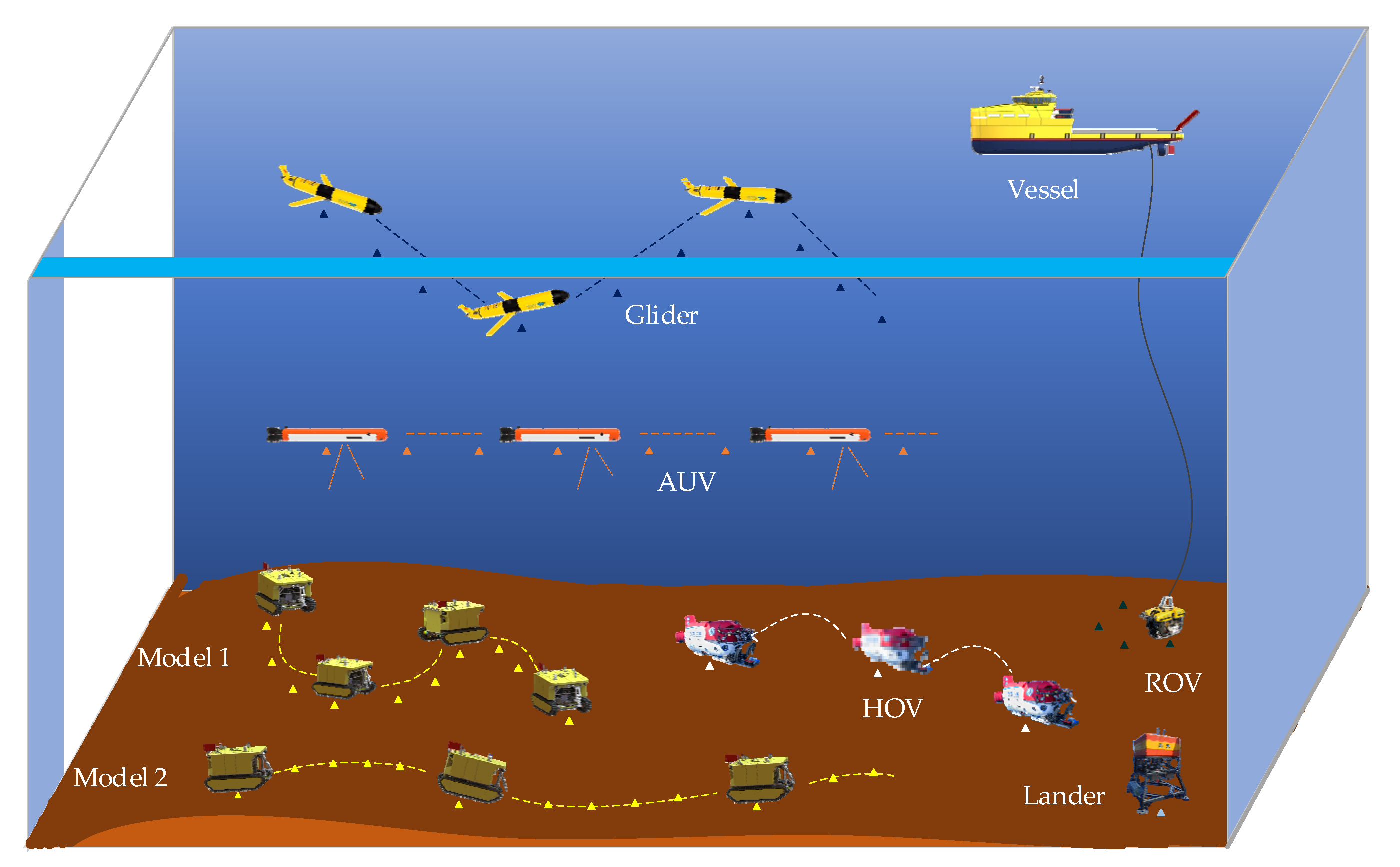
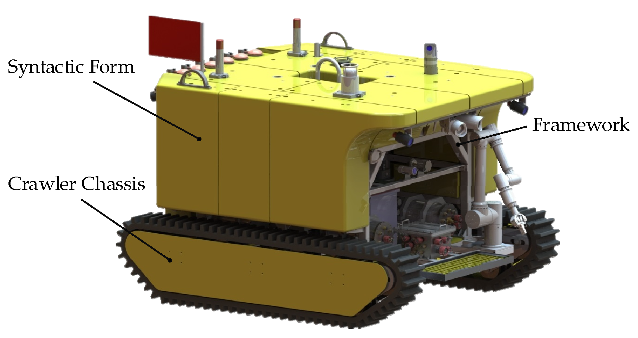
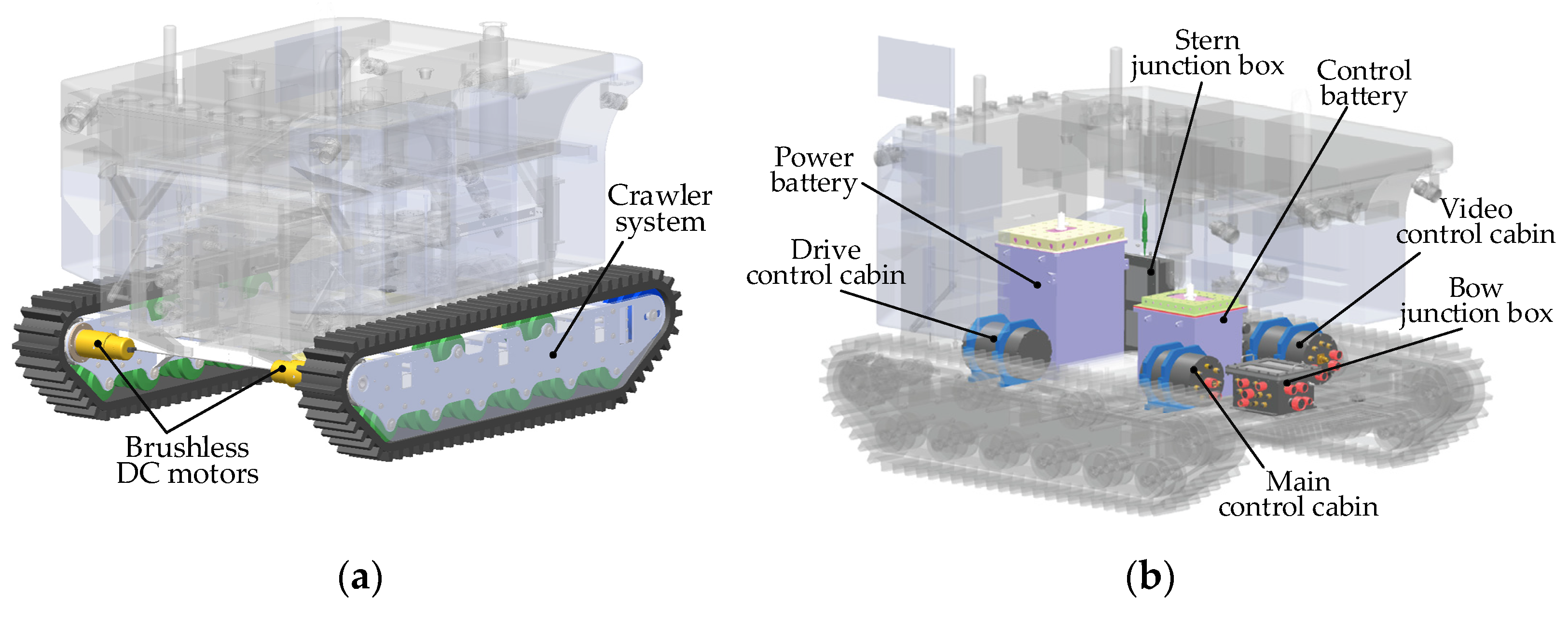
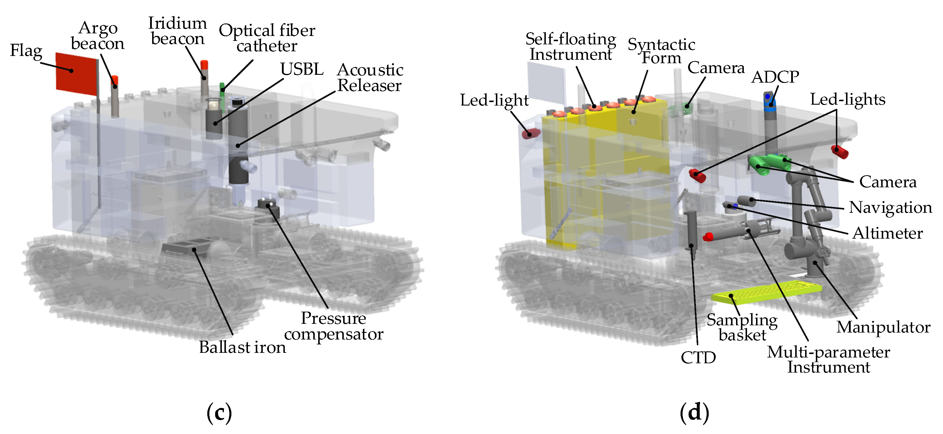
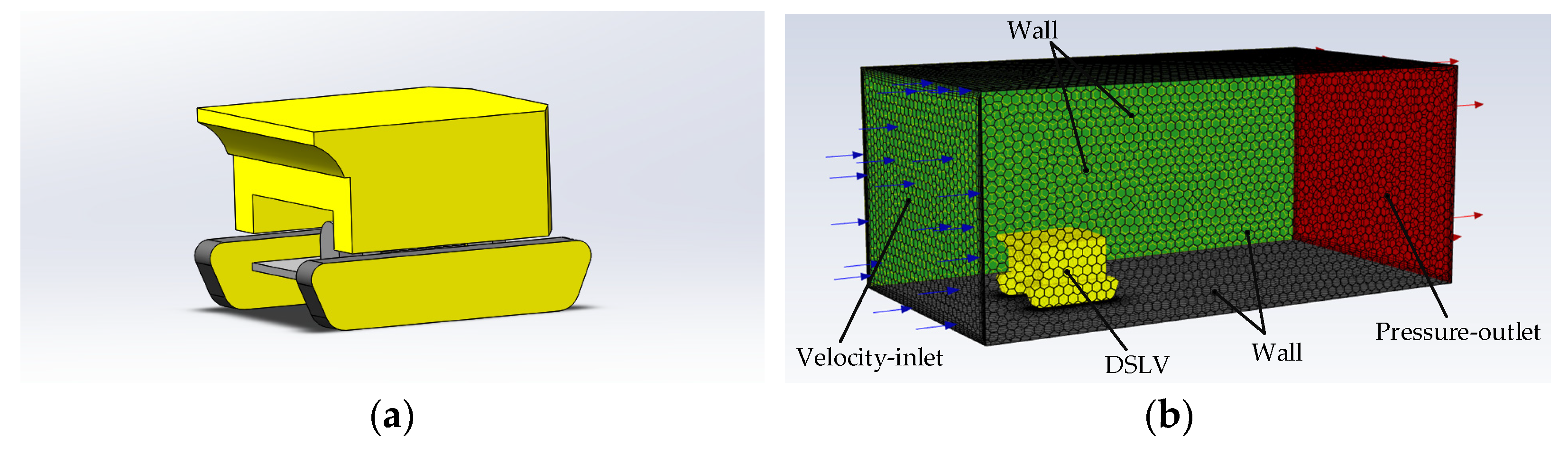
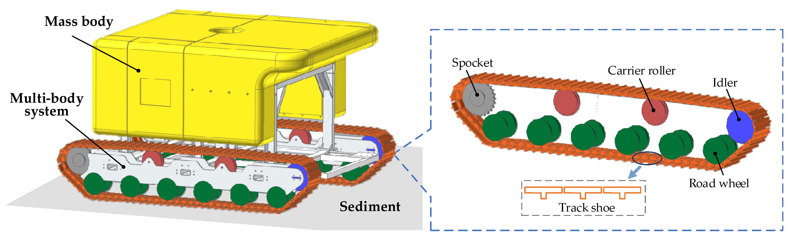
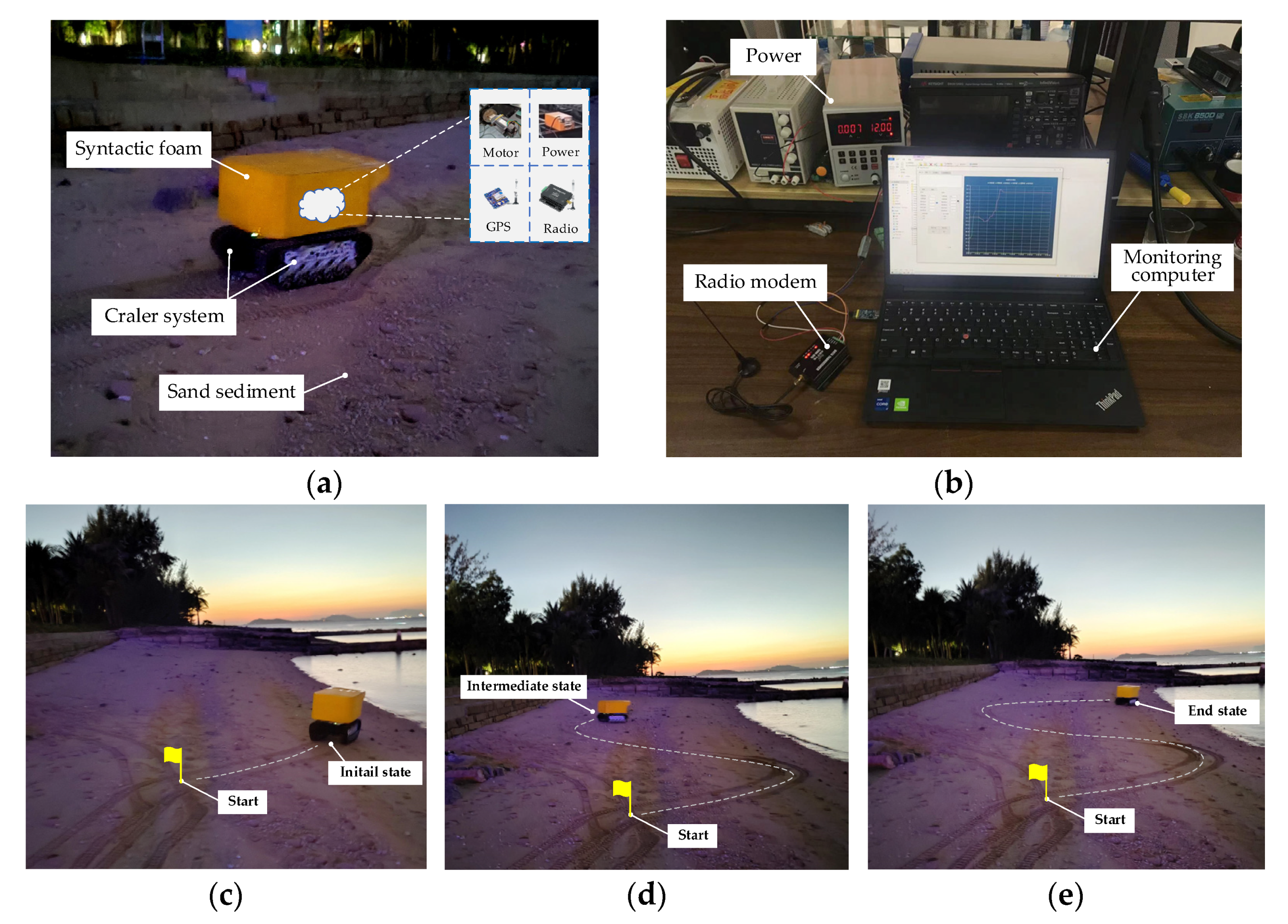
2.1. Conceptual Prototype Design of DSLV

The DSLV, in which crawler chassis and function components are integrated, is designed as a universal transporting platform to ensure stable operation, instrument delivery, and intelligent expansion, as displayed in Figure 2. The conceptual prototype has dimensions of 2.2 m × 1.6 m × 1.3 m, and the maximum design depth of the vehicle is 4500 m. The prototype has a plurality of syntactic foam, which can provide buoyancy wrapped around the titanium component framework. The vehicle weighs 1600 kg in air and has approximately 50 kg of negative buoyancy in seawater; specifically, the actual value of negative buoyancy can be designed according to the various requirements of special scientific research tasks. The modular design of functional components facilitates the autonomy and expansibility of each electrical subsystem, so the modular subsystems for docking and scientific payload can be added depending on various scientific requirements. However, considering the minimum hydrodynamic resistance, the lightest structural weight, maximum scientific load expansion, and outstanding trafficability are basic requirements that should be achieved during prototype development.

As a powerful carrier platform for autonomous mobile scientific research on the seafloor, DSLV consists of four major subsystems, namely, chassis drive and crawling systems; energy and electronic systems; location and recovery systems; scientific payload and communication systems. As displayed in Figure 3a, the crawler assemblies are used as the chassis walking structure to ensure the passage of the vehicle on the seafloor. All of its moving parts are made of polyethylene, including crawlers, wheel sets, fenders, and bearings, in which the fenders avoid the crawler track blockage by the rocks. Each crawler system is driven by a DC brushless motor with a 1:160 reduction in spur gear, a voltage of 110 V, and a power of 450 W. As the customised motor and reducer are installed in a sealed cabin filled with hydraulic oil and surrounded by a high-pressure environment, the driving efficiency is only maintained in the range of 50–70%.

As displayed in Figure 3b, the system is supplied by the control and power lithium batteries, the electronic equipment and control system are powered by a 24 V control battery pack (capacity of 6.5 kWh), and the brushless motor and manipulator are powered by a 110 V power battery (capacity of 13.5 kWh). The control system includes a main control core, a drive control core, a video control core and corresponding peripheral circuits. The three aforementioned control cores are used to realise the information exchange based on the CAN bus. The design of the bow and stern junction boxes facilitates the overall system layout and function expansion.

As displayed in Figure 3c, after completing an investigation mission, the 120 kg ballast iron equipped with the vehicle is released according to the combined command of the passive motor and active acoustic releaser. The ballast iron state is measured by the detection sensor in real time, and the main control core performs remedial measures based on the detection information. After releasing the ballast iron, the vehicle float sup to the sea surface with a positive buoyancy of approximately 70 kg in a stern cocking attitude. Researchers have combined the positions provided by the argo beacon, the iridium beacon, and the flag to complete recovery.

As displayed in Figure 3d, the LED lights and cameras installed at the bow and stern were combined with an optical fibre to form an observation and communication system, which can upload the seafloor video to the vessel monitoring terminal in real time. Multiple sensors on the vehicle, including ADCP, CTD, Altimeter, and navigation sensors, can obtain multi-dimensional environmental information for scientific research. As the six self-floating instruments can intermittently transmit the data for multi-parameter sensors, including temperature, salinity, pressure, turbidity, and chlorophyll, to the sea surface, and send them to the laboratory via Beidou satellite, we obtained a 6-month seafloor environment changing in real-time as much as possible. In addition, the manipulator can also collect interested samples, such as soft-bodied organisms, metal mineral nodule, sediments, and store them in the sampling basket and transport them to the vessel. All the aforementioned data can be stored and decided locally to realise the real-time remote control with vessel through the micro-fibres.

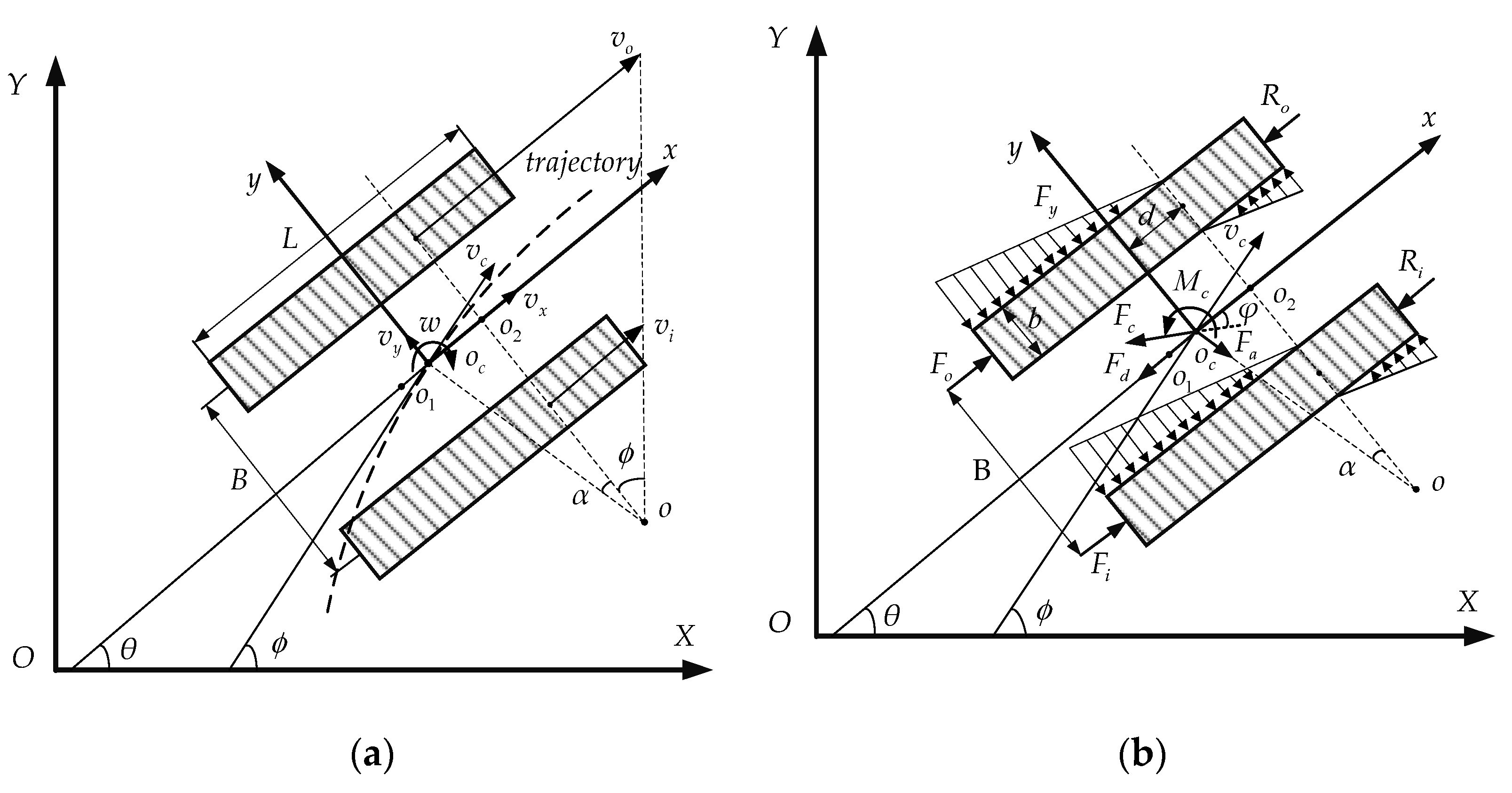
2.2. Motion Model of Black-Box

According to the aforementioned description, the DSLV mainly performs continuous linear motions on the seafloor over a wide area and multi-angle steering motions in a local area. Before analysis of the motion, three basic assumptions were made:

• The carrier of the vehicle exhibits a symmetrical structure with respect to its longitudinal and transverse axes;
• The coordinate position of the vehicle’s mass centre coincides with the geometric centre of the carrier structure;
• The seafloor is flat in the local area, and motion analysis can be based on a two-dimensional plane.

Generally, the vehicle motion on the geographic coordinate system O-XY includes: forward, sideshift, heave, pitch, roll and yaw, but because the seafloor was considered to be flat, only forward, sideshift, and yaw were considered. The design and installation ensure that the origin $o_c$ of the carrier coordinate system $o_c\text{-}\mathrm{xy}$ always coincides with the mass centre of the vehicle, and the motion coordinate system and the carrier coordinate system also completely coincide.

When DSLV changes from a linear motion to a steering motion, its instantaneous steering centre does not coincide with the mass centre of the carrier. As displayed in Figure 4, when the lateral force $F_y$ is zero, $o_1$ is considered the centre point of instantaneous steering. Next, the vehicle has a certain forward speed, and the steering centre moves forward from $o_1$ to $o_2$ to generate sufficient lateral force to balance the centrifugal force caused by carrier steering. Because of the separation of $o_2$ and $o_c$, the instantaneous velocity $v_c$ produces a lateral slip angle α, and the figure clearly shows that when point $o_2$ is behind $o_c$, the lateral velocity of the centre of mass points from the outside to the inside of the track, when the point $o_2$ is in front of $o_c$, the lateral velocity of the centre of mass points from the inside to the outside of the track.

The kinematic analysis of the vehicle motion process as displayed in Figure 4a. The vehicle motion on the O-XY of the geographic coordinate system can be considered as the synthesis of the forward motion with the centroid velocity $v_c$ and the steering motion with the angular velocity $w$, where $v_x$ and $v_y$ represent the decomposition variables of $v_c$ on x axis and y axis, respectively, and the vehicle direction angle and the position relative to O-X axis of the geographic coordinate system are represented by φ and θ, respectively. The kinematic analysis equation is expressed as:

$$\{\begin{array}{l}\dot{x}=v_x\cos \theta +v_y\sin \theta \\ \dot{y}=v_x\sin \theta +v_y\cos \theta \\ \dot{\theta }=w\end{array}$$

(1)

In the dynamic analysis of the vehicle motion process, as shown in Figure 4b, $F_i$ and $F_o$ represent the seafloor sediments’ traction resistance of the inner and outer crawlers, respectively, $R_i$ and $R_o$ represent the seafloor sediments rolling resistance of the inner and outer crawlers, respectively, $F_f$ is the deep-sea current interference force, $F_d$ is the hydrodynamic resistance opposite to the motion direction, and the movement process is also affected by lateral resistance $F_y$ and resistance torque $M_c$. The dynamics analysis equation is expressed as:

$$\{\begin{array}{l}m{\dot{v}}_x=F_o+F_i-R_o-R_i-F_d-F_c\cos \phi +m{w}^{2}R\sin \alpha \\ m{\dot{v}}_y=F_f\sin \phi -m{w}^{2}R\cos \alpha -F_y\\ I_c\dot{w}=B\left(F_o-F_i\right)/2-B\left(R_o-R_i\right)/2-M_c\end{array}$$

(2)

where m and $I_c$ epresent the mass of the vehicle in water and the moment of inertia around the mass center, respectively.

According to motion analysis, the model relationship can be expressed as follows:

$$\{\begin{array}{l}\dot{\mathit{x}}=\mathit{R}(\mathit{x}) \mathit{q}\\ \dot{\mathit{q}}=f(F_o,F_i, \mathit{q})\end{array}$$

(3)

where $\mathit{x}={[x,y,\theta ]}^T$ represent the position and path angle in geographic coordinate system; $\mathit{q}={[v_x,v_y,w]}^T$ represent the velocity and angular velocity in the motion coordinate system; $\mathit{R}(\mathit{x})$ is the conversion matrix between the motion coordinate system and geographic coordinate system.

The motion state can be obtained at any time according to Equation (3); however, because of the discontinuity in the motion measurement, the discrete time model can be used to replace the continuous time model.

$$\{\begin{array}{l}\dot{\mathit{x}}(t)=(\mathit{x}(t+1)-\mathit{x}(t))/\Delta t\\ \dot{\mathit{q}}(t)=(\mathit{q}(t+1)-\mathit{q}(t))/\Delta t\end{array}$$

(4)

where $\Delta t$ is the interval of discrete time, t and t + 1 represent the adjacent sampling movements around the motion state of the vehicle.

Combining Equations (1)–(4), the motion state of the vehicle at time k + 1 can be expressed as follows:

$$\{\begin{array}{l}\mathit{x}(t+1)=\mathit{x}(t)+\mathit{R}(\mathit{x}(t))\mathit{q}(t)\Delta t\\ \mathit{q}(t+1)=\mathit{q}(t)+f(F_o(t), F_i(t), \mathit{q}(t))\Delta t\end{array}$$

(5)

where sediment resistance, hydrodynamic resistance, current interference and resistance torque were determined by the environment in which the vehicle was located, while the mass and the moment of inertia are related to the structural design. Therefore, the position and velocity of DSLV at time t + 1 can be obtained according to the position, velocity, and driving force at time t, which is described as follows:

$$\begin{array}{l}x (t+1)=g_1(x(t),y(t),\mathsf{\theta }(t),v_x(t),v_y(t),w(t),F_o(t),F_i(t))\\ y (t+1)=g_2(x(t),y(t),\mathsf{\theta }(t),v_x(t),v_y(t),w(t),F_o(t),F_i(t))\\ \theta (t+1)=g_3(x(t),y(t),\mathsf{\theta }(t),v_x(t),v_y(t),w(t),F_o(t),F_i(t))\\ v_x(t+1)=g_4(x(t),y(t),\mathsf{\theta }(t),v_x(t),v_y(t),w(t),F_o(t),F_i(t))\\ v_y(t+1)=g_5(x(t),y(t),\mathsf{\theta }(t),v_x(t),v_y(t),w(t),F_o(t),F_i(t))\\ w (t+1)=g_6(x(t),y(t),\mathsf{\theta }(t),v_x(t),v_y(t),w(t),F_o(t),F_i(t))\end{array}$$

(6)

The nonlinear mapping relationship between the motion states and driving force can be established according to Equation (6). In following sections, the black-box modelling method and the data-driven model will be realised, and the time series prediction of the motion state can be achieved under typical driving forces.

3. Black-Box Modelling Method

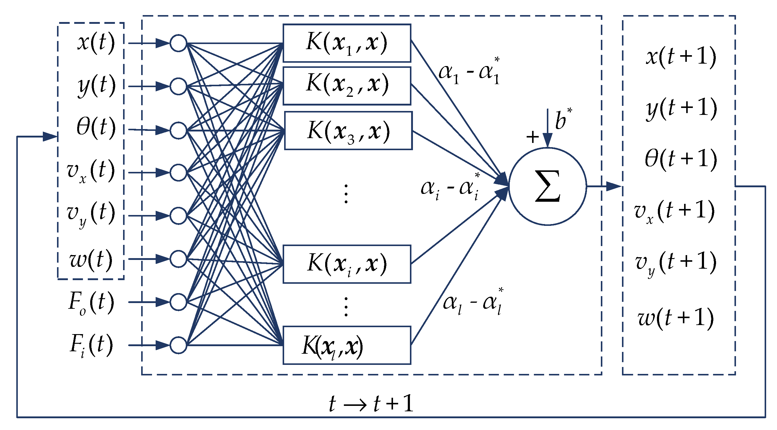
3.1. Support Vector Regression

SVM is a machine learning algorithm based on the statistical learning theory created by Vapnik, which can complete the generalised linear classification of high-dimensional supervised learning with limited samples [18]. SVM is an excellent classifier with sparsity and robustness and has been successfully applied to numerous engineering cases of nonlinear regression estimation. To solve the non-separability of lower-dimensional data, the kernel function was introduced to obtain a higher-dimensional nonlinear mapping of lower-dimensional samples, which allows for nonlinear SVM classification and avoids data dimension disasters.

To investigate universality, supposing separable datasets $\{({\mathit{x}}_i,y_i),i=1,2,\cdots ,l\}$ are given as training samples, the vectors ${\mathit{x}}_i={(x_{i1},x_{i2},\cdots ,x_{iD})}^T$ is the column vector of the i-the training sample, where l is the number of training samples, D is the dimension of the input sample vectors, and $y_i=\pm 1$, which is denoted as the class label of the predicted result. If the samples in the same category can be divided into the same side by the hyperplane $\mathit{w}{\mathit{x}}_i+b=0$, the SVM classification is abstracted as the relationship of Equation (7).

$$\{\begin{array}{l}\mathit{w}{\mathit{x}}_i+b\ge 1,\hspace{1em}\hspace{1em}{y}_i=1\\ \mathit{w}{\mathit{x}}_i+b\le -1,\hspace{1em}{y}_i=-1\end{array}$$

(7)

where w and b are the weight coefficient matrix and linear bias, respectively. Then, the classification problem can be expressed abstractly as solving an optimisation function that maximizes the sample interval $y_i(\mathit{w}{\mathit{x}}_i+b)$, and is a convex optimisation problem, as described in Equation (8).

$$\{\begin{array}{l}\underset{\mathit{w},b}{\min } \frac{1}{2}{\Vert \mathit{w}\Vert }^2\\ \mathrm{s}.\mathrm{t}. y_i(\mathit{w}{\mathit{x}}_i+b)\ge 1\end{array}$$

(8)

According to Equation (8), a hyperplane $\mathit{w}{\mathit{x}}_i+b=0$ with the largest margin can be obtained, while the prediction of motion state needs to introduce an insensitive loss factor $\epsilon$ based on SVM. Considering the datasets’ linear inseparability in higher-dimensional space, the slack factors ${\xi }_i$ and ${\xi }_i^{\ast }$ are introduced to the optimisation problem. Then, SVR is formulated as a convex optimisation problem, which is described in Equation (9).

$$\{\begin{array}{l}\underset{\mathit{w},b}{\min } \frac{1}{2}{\Vert \mathit{w}\Vert }^2+C{\displaystyle \sum _{i=1}^l({\xi }_i+{\xi }_i^{\ast })}\\ \mathrm{s}.\mathrm{t}. \{\begin{array}{l}{y}_i-(\mathit{w}\varphi (x_i)+b)\le \epsilon +{\xi }_i\\ \mathit{w}\varphi ({\mathit{x}}_i)+b-y_i\le \epsilon +{\xi }_i^{*}\\ {\xi }_i\ge 0, {\xi }_i^{*}\ge 0\end{array}\end{array}$$

(9)

where the penalty coefficient C is used to constrain the slack variable factors, aiming to prevent the factors ${\xi }_i$ and ${\xi }_i^{\ast }$ from being too large and reducing the modelling accuracy.

The most commonly used method is to combine the constructed Lagrangian function to transform the constrained function into an unconstrained function based on the convex optimisation problem [19]. In this case, the dual problem can be defined as a maximized quadratic programming problem, as described in Equation (10).

$$\{\begin{array}{l}\underset{\alpha ,{\alpha }^{\ast }}{\max } [-\frac{1}{2}{\displaystyle \sum _{i=1}^l{\displaystyle \sum _{j=1}^l({\alpha }_i-{\alpha }_i^{\ast })({\alpha }_j-{\alpha }_j^{\ast })K({\mathit{x}}_i,{\mathit{x}}_j)-{\displaystyle \sum _{i=1}^l({\alpha }_i+{\alpha }_i^{\ast })\epsilon +{\displaystyle \sum _{i=1}^l({\alpha }_i-{\alpha }_i^{\ast })y_i}}}}]\\ \mathrm{s}.\mathrm{t}. \{\begin{array}{l}{\displaystyle \sum _{i=1}^l({\alpha }_i-{\alpha }_i^{\ast })=0}\\ 0\le {\alpha }_i\le C , 0\le {\alpha }_i^{\ast }\le C\end{array}\end{array}$$

(10)

where $K({\mathit{x}}_i,{\mathit{x}}_j)=\varphi ({\mathit{x}}_i)\cdot \varphi ({\mathit{x}}_j)$ denotes the kernel function, $\varphi (\mathit{x})$ denotes the higher dimensional feature mapping of the sample $\mathit{x}$, $\mathit{\alpha }$ and ${\mathit{\alpha }}^{\ast }$ denote the Lagrangian coefficient vectors, which can be calculated using the sequential minimal optimization (SMO) to solve quadratic programming problems.

According to Karush–Kuhn–Tucker (KKT) conditions [20], the solution to Lagrange function can be expressed as Equations (11) and (12).

$${\mathit{w}}^{\ast }={\displaystyle \sum _{i=1}^l({\alpha }_i-{\alpha }_i^{\ast })\varphi ({\mathit{x}}_i)}$$

(11)

$$b^{\ast }=\frac{1}{N}\left\{{\displaystyle \sum _{{\alpha }_i}\left[y_i-{\displaystyle \sum _{x_i}({\alpha }_i-{\alpha }_i^{\ast })K({\mathit{x}}_i,{\mathit{x}}_j)-\epsilon }\right]+{\displaystyle \sum _{{\alpha }_j}\left[y_i-{\displaystyle \sum _{x_j}({\alpha }_j-{\alpha }_j^{\ast })K({\mathit{x}}_i,{\mathit{x}}_j)+\epsilon }\right]}}\right\}$$

(12)

where N is the number of support vectors, and the regression function established in the higher-dimensional feature space:

$$f(\mathit{x})={\mathit{w}}^{\ast }\varphi (\mathit{x})+b^{\ast }={\displaystyle \sum _{i=1}^l({\alpha }_i-{\alpha }_i^{\ast })K({\mathit{x}}_i,\mathit{x})+b^{\ast }}$$

(13)

where $f(\mathit{x})$ is the motion-predicted value, and the linear combination of intermediate nodes is similar to that of the neural network. The structure of SVR modelling and prediction is displayed in Figure 5.

The selection of a kernel function affects the model generalization because SVR is a kenel-based algorithm [21]. Generally, kernel functions are linear function, d-order polynomial function, sigmoid function with parameters k and θ, and Radial Basis Function (RBF). Among them, RBF, as described in Equation (14) and applied in this paper, is the most commonly used.

$$K({\mathit{x}}_i,\mathit{x})=\exp (-\frac{{\Vert \mathit{x}-{\mathit{x}}_i\Vert }^2}{2{\mathsf{\sigma }}^2})$$

(14)

where σ represents the Gaussian kernel bandwidth, and if its value is excessively large or small, it leads to overfitting or underfitting.

3.2. Particle Swarm Optimisation

The basic idea of PSO is that particles are initialised in the feasible region, and the potential result is represented by the particle position. In each iteration, the position and velocity will be updated with a certain law [22]. The fitness calculated by the fitness function is used to describe the advantages and disadvantages of the solution to determine whether the algorithm has obtained the optimal value.

Suppose initial particles are described as matrix $\mathit{x}=({\mathit{x}}_1,{\mathit{x}}_2,\cdots ,{\mathit{x}}_n)$ in D-dimensional feasible region, the abstract position of the i-th particle in space is expressed as a vector ${\mathit{x}}_i={(x_{i1},x_{i2},\cdots ,x_{\mathrm{iD}})}^T$, in which ${\mathit{x}}_i$ can be considered as a potential solution. Next, fitness is also solved by the fitness function according to the vector ${\mathit{x}}_i$. Furthermore, the velocity of the i-th particle is represented by a vector ${\mathit{v}}_i={(v_{i1},v_{i2},\cdots ,v_{iD})}^T$, and the vector ${\mathit{p}}_i={(p_{i1},p_{i2},\cdots ,p_{iD})}^T$ and vector ${\mathit{p}}_g={(p_{g1},p_{g2},\cdots ,p_{gD})}^T$ are represented as the individual and group optimal values, respectively.

The velocity and position of the particles are iterated as follows:

$$v_{\mathrm{id}}^{k+1}=w{v}_{id}^k+c_1{r}_1(p_{id}^k-x_{id}^k)+c_2{r}_2(p_{gd}^k-x_{id}^k)$$

(15)

$$x_{id}^{k+1}=x_{id}^k+v_{id}^{k+1}$$

(16)

where w is the inertia weight coefficient, $d=1,2,\cdots ,D$,$i=1,2,\cdots ,n$, and k represents the number of iterations of the current algorithm, $c_1$ and $c_2$ are nonnegative acceleration constant factors, and $r_1$ and $r_2$ are random numbers distributed between 0 and 1.

Furthermore, parameter w was named the inertia weight coefficient, which reflects the particles’ ability to inherit the previous speed. A large inertia weight is conducive to the global search of particles, and the local search ability’s excellent performance depends on a smaller weight. Then, a linearly decreasing inertia weight coefficient was adopted in this paper. The specific equation is as follows:

$$w(k)=w_{\mathrm{start}}+\left(w_{\mathrm{start}}-w_{\mathrm{end}}\right)\left[\frac{2k}{T_{\max }}-{\left(\frac{k}{T_{\max }}\right)}^2\right]$$

(17)

where $w_{\mathrm{start}}$ and $w_{\mathrm{end}}$ represent the inertia weight at beginning and maximum iterated number, respectively, $T_{\max }$ is the maximum iterated number, and the comprehensive performance of PSO is the best when inertia weight $w_{\mathrm{start}}$ = 0.9 and $w_{\mathrm{end}}$ = 0.4.

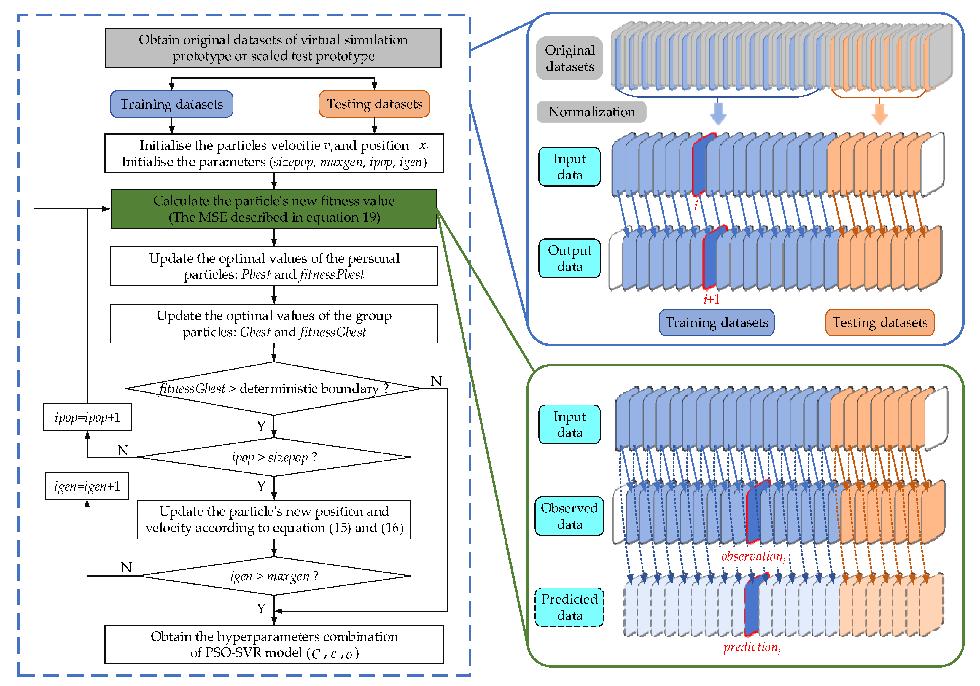
3.3. SVR Optimised by PSO

Machine learning based on kernel function can achieve a nonlinear mapping of high-dimensional feature spaces, while hyperparameter combinations have not been comprehensively theoretically studied. In this section, the PSO with an extremely powerful multiparameter optimisation ability was used to resolve hyperparameter optimisation, and we focused our modelling and prediction on time series with a strong generalisation ability between driving forces and motion states. The flowchart of PSO–SVR modelling and prediction framework is displayed in Figure 6.

An accurate motion model is established based on obtaining hyperparameter combinations, including penalty coefficient C, loss factor $\epsilon$ and Gaussian kernel σ. The main research ideas of this framework are as follows.

• Step 1. Obtain training and testing datasets

The virtual prototype including hydrodynamic resistance $F_d$, current interference $F_f$ and nonlinear seafloor sediments was established, and the 2:1 scaled test prototype was developed in combination with its conceptual prototype (in Section 4); next, we considered the motion states x and q, which were obtained under $F_o$ and $F_i$ as original datasets.

To improve model prediction accuracy and smooth the training procedure, the scattered and large-span datasets should be normalised. The following linear mapping formula was used to map the data in the interval [0, 1]:

$$x^{\prime }=\frac{x_i-x_{\min }}{x_{\max }-x_{\min }},\hspace{1em}i=1,2,3\cdots N$$

(18)

where $x^{\prime }$ is the mapped value, $x_i$ is the i-th input data, $x_{\min }$ and $x_{\max }$ are the minimum and maximum values of the original data, respectively, and N is the total number.

The N datasets were divided into two sample groups after normalization with the K and N-K-1 numbers based on a given ratio. Because the two groups of samples obtained are one-dimensional arrays, and the i-th data and +1-th data of the two sample groups were referred to as input samples and output samples, respectively, as displayed in Figure 6 to form training and testing datasets with time series characteristics. These datasets were used to complete the black-box modelling and time series prediction.

• Step 2. Initialise particle population

Before iterative optimisation, the population size sizepop, the maximum iteration number maxgen, and the deterministic boundary should be initialised, and the random value and limit boundary of the particle velocities ${\mathit{v}}_i$ and positions ${\mathit{x}}_i$ should be given. Among them, the parameters of penalty coefficient C, loss factor $\epsilon$, and gaussian kernel σ in the framework were set as the three-dimensional parameters of position x.

• Step 3. Calculate the fitness value of the particles

The fitness value in the PSO represents the relative distance between the current particle position and the final food position. In this model framework, we set the mean square error (MSE) between the observed and predicted values of l samples of the motion states as the abstract fitness value. The equation for MSE was as follows:

$$\mathrm{MSE}=\frac{1}{l}{\displaystyle \sum _{i=1}^l{({\mathit{observation}}_i-{\mathit{prediction}}_i)}^2}$$

(19)

• Step 4. Update particles position and velocity

The initial group consists of particles with a random position and random velocity; the fitness value of each particle was described in Equation (19). When the particle updated the position each time, the fitness value was calculated once. If the fitness value of the new position of the particle was better than its personal historical optimal value, the personal optimal value Pbest was updated. If the fitness value of the new position of the particle was better than the group optimal value, then the new group optimal Gbest could be recorded.

• Step 5. Assessing the convergence of hyperparameters

According to the update principle in step 4, the particles’ velocities ${\mathit{v}}_i$ and positions ${\mathit{x}}_i$ were updated until the termination condition was satisfied. In this model framework, we set the group optimal fitness value to fitnessGbest less than the deterministic boundary and the number of iterations ipop beyond the maximum given value sizepop as the criterion for the convergence; next, we finally obtained the hyperparameter combination of the PSO–SVM model.

4. Validation of the Algorithm

To verify the predictive ability of the black-box model based on the proposed PSO-SVR, the data obtained from the virtual prototype and the scaled test prototype were combined to confirm the rationality and provide the theoretical method and data support. The virtual prototype is affected by complex factors, including hydrodynamic resistance, current interference, and seafloor sediment. During the simulation, the seafloor environment should be restored as much as possible to obtain accurate motion information with constant and variable driving forces. Finally, the nonlinear mapping relationship between the driving force and motion state was established, and the time-series prediction and robustness of the model were verified by the 2:1 scaled test prototype.

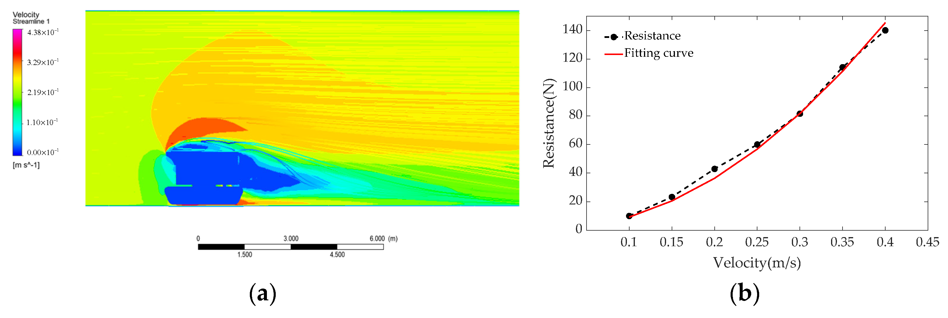
4.1. Hydrodynamic Resistance and Current Interference

Before the simulation motion of the virtual prototype is realised, analysing and calculating the hydrodynamic resistance $F_d$ and the current interference $F_c$ described in Equation (2) are critical factors in simulating a realistic seafloor environment to establish a precise black-box model. When DSLV moves on the seafloor, the incompressible fluid around it produces a hydrodynamic resistance dominated by friction resistance, its numerical results are closely related to its fluid density, wet surface area, and relative velocity, and the direction of hydrodynamic resistance is opposite to its relative motion. The parameter influence relationship can be described as follows:

$$F_d=\frac{1}{2}\rho C_{d}S{v}_c^2$$

(20)

where ρ is the density of 4500 m seawater with 1047 kg/m³, S is the prototype wet surface area with 1.77 m², and $C_d$ is the resistance coefficient of the conceptual prototype.

As displayed in Figure 7a, to satisfy the CFD method requirements, the DSLV 3D model was simplified as follows: (1) on the basis of ensuring the shape characteristics, the functional components carried by the vehicle were removed to reduce the finite-element model complexity; (2) the complex structure was simplified to improve mesh quality for model analysis, including the frame, track wheels, and auxiliary installation structure. Figure 7b displays the 3D model computational domain of the vehicle. To ensure the expansion of the water flow, the design size of the flow field is 2 L in the front and 4 L in the rear (where L represents the body length), and the DSLV was close to the lower wall to simulate the seafloor.

The hydrodynamic resistance $F_d$ versus the velocities of 0.1, 0.15, 0.2, 0.25, 0.3, 0.35, and 0.4 m/s were calculated using the RNG k–ε turbulence model in software Fluent. Figure 8 displays the calculated results of the resistance and the fitted curve of Equation (20). The resistance coefficient $C_d$ was identified by the least square with a value of 0.981.

Ocean observation data in the South China Sea confirm that the current velocity at the surface and subsurface is typically the strongest, and the velocity of the current near the middle layers and seafloor considerably decreases [23]. Then, the analysis process complexity was simplified on the basis of ensuring the most realistic restoration of the current interference on the seafloor. The current interference $F_c$ can be regarded as a constant value in the virtual prototype simulation process [9]. Combined with the current observation in the South China Sea and the hydrodynamic simulation results in Figure 8b, the current interference of the DSLV while crawling on the seafloor was set to 25 N.

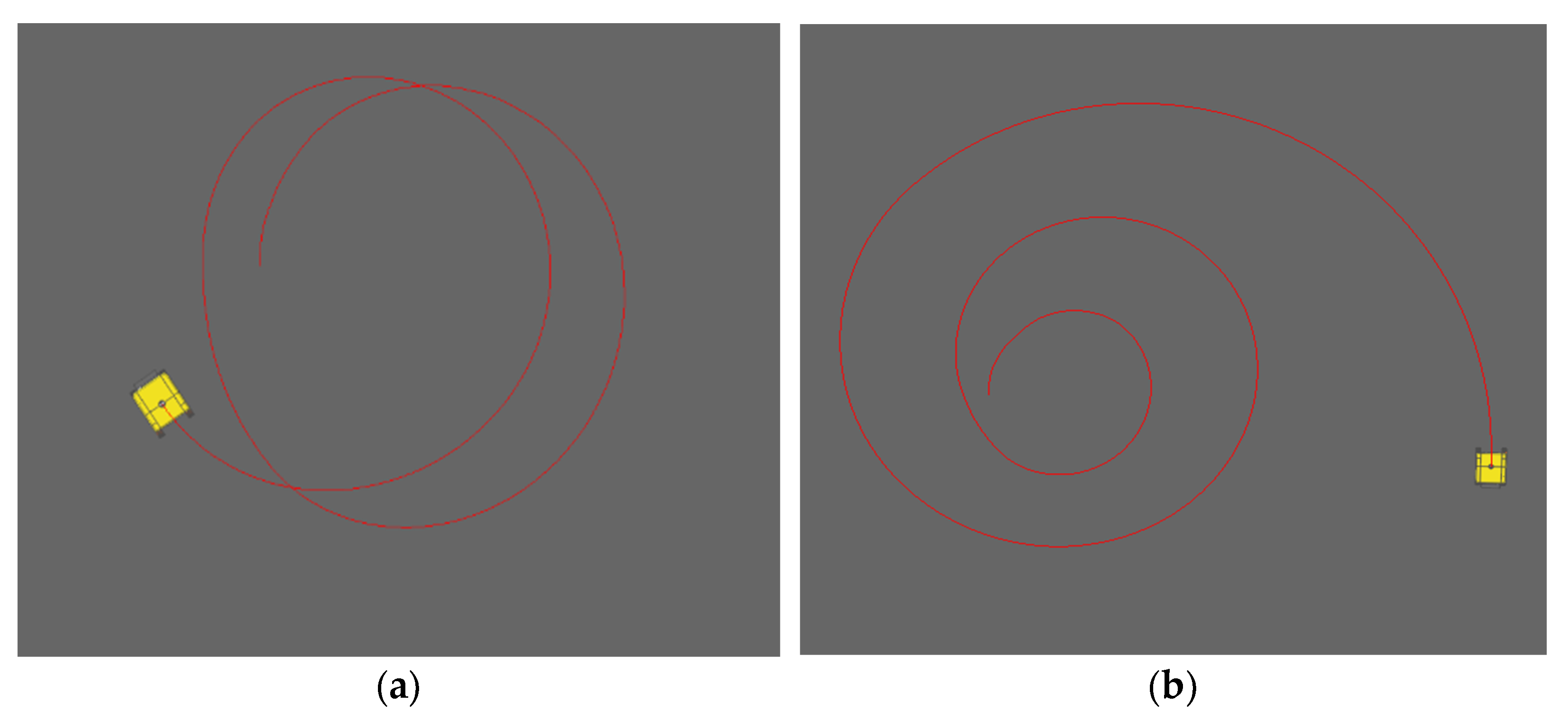
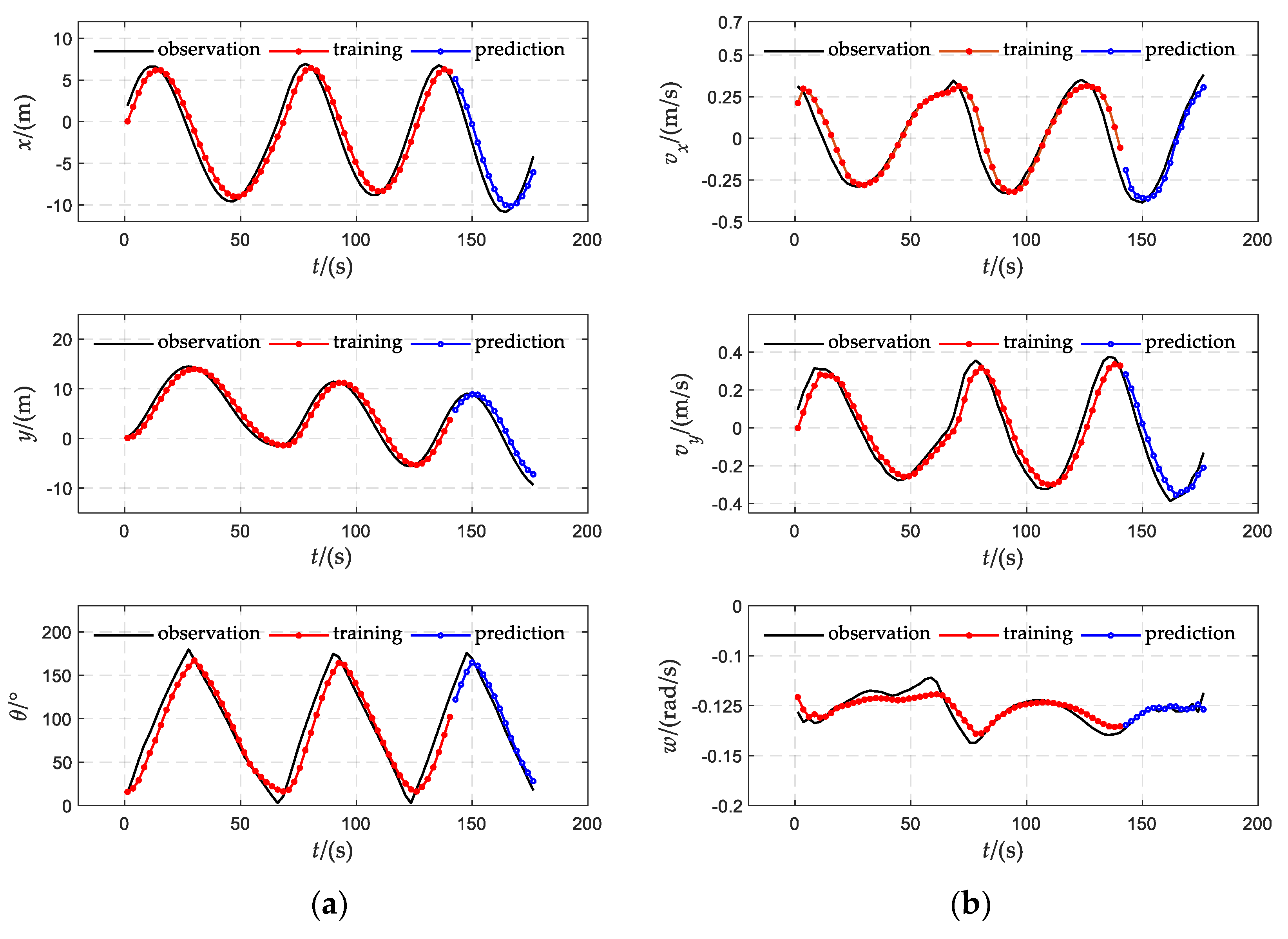
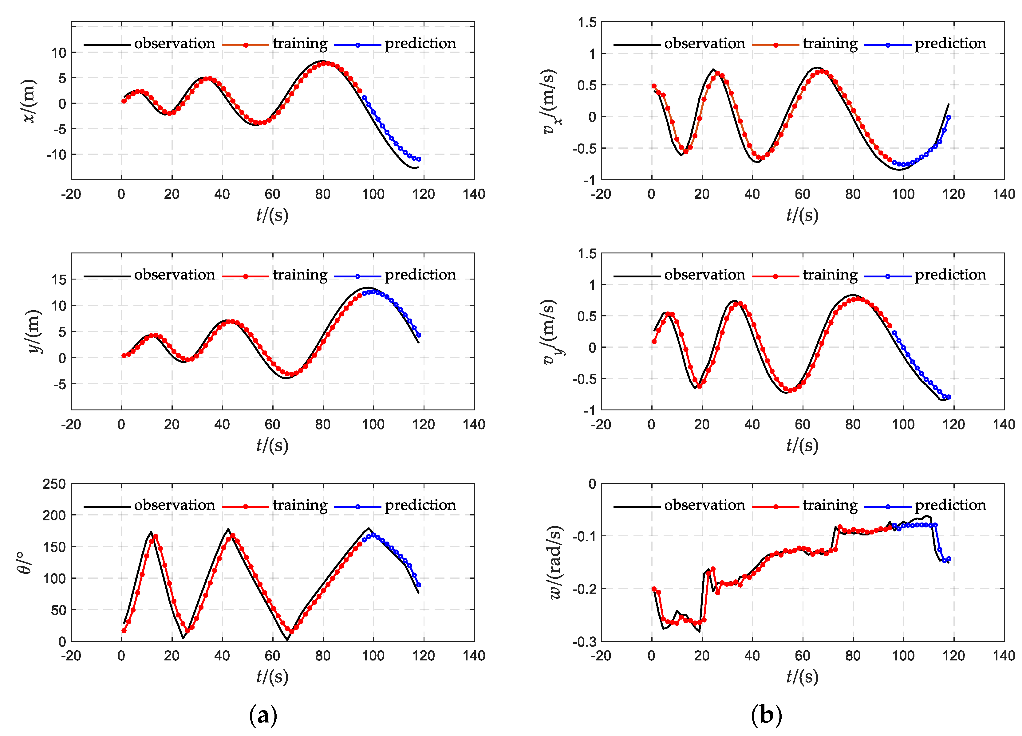
4.2. Simulation of the Virtual Prototype

In addition to hydrodynamic resistance $F_d$ and current interference $F_c$, the vehicle motion state is affected by complex nonlinear mechanical properties, such as the friction loss of the crawler system, the rubber track winding elastic resistance, and the interaction resistance between the crawler and sediments during crawling on the seafloor. The structural model described in Figure 9 was simplified according to the vehicle’s basic structural and design parameters. The crawler systems, including the spocket, road wheel, idler, carrier roller, and track shoe, were established in combination with the actual movement. The buoyancy, hydrodynamic resistance, and current interference generated by the vehicle were considered in the virtual simulation prototype.

When the DSLV travels on the seafloor sediments, it causes a typical elastic–plastic deformation, with the elastic deformation dominating [24]. Various parameters, such as the shoe structural shape, vehicle driving speed, sediment layered structure, and sediment components, influence the mechanical characteristics of seafloor sediments. Therefore, while evaluating the vehicle mechanical model and sediments, the nonlinear mechanical form was provided. The nonlinear sediment was simulated using relevant research [5,25], while the sediment simulation parameters were selected as in

Table 1. Sediment parameters of the simulation model of DSLV.

Parameter	Value
$\mathrm{Terrain} \mathrm{Stiffness} (k_c$)	0.4171
$\mathrm{Terrain} \mathrm{Stiffness} (k_b$)	0.012
Exponential Number (n)	0.7
Cohesion (c)	0.00172
Shearing Resistance Angle	29
Shearing Deformation Modulus (k)	25
Sinkage Radio	0.05

based on the description in commercial software RecurDyn [26], and the vehicle motion state on the seafloor may be restored to the highest possible degree.

The study of the black-box model was based on the motion state under various driving forces. The goal was to validate the generalisation abilities of the algorithm framework proposed in this paper by considering both constant and variable driving forces. Figure 10a displays the motion trajectories when the inner and outer crawler drive functions were set to STEP (Time, 0, 0, 0.01, 50) and STEP (Time, 0, 0, 0.01, 80), respectively. When the driving forces were at a constant value, due to the influence of nonlinear sediments’ mechanical properties and lateral current interference, the DLSV formed a lateral helical motion with a certain radius. Figure 10b displays the motion trajectory when the inner and outer crawler driving forces were set to STEP (Time, 0, 0, 0.01, 50) + STEP (Time, 0.1, 0, 20, 30) and STEP (Time, 0, 0, 0.01, 100) + STEP (Time, 0.1, 0, 20, 30), respectively. When the driving forces were variable value, the DSLV makes a spiral motion with an increasing radius because the variable driving forces’ influence was greater than that of the nonlinear disturbance.

The state quantities $\mathit{x}(t)$, $\mathit{q}(t)$ were obtained when the driving force was constant and variable, respectively, and the six variables described in Equation (6) were modelled and predicted according to the flowchart displays in Figure 6. According to the simulation experiments, the smoothed sample datasets were sampled at intervals, and the i-th data and the i+1-th data were combined to obtain a time series dataset. The first 70% of the motion simulation data were used as the training datasets to establish the black-box model of the variables in the time series, and the last 30% of the motion simulation data were used as the testing datasets to verify the prediction accuracy of the variables in the time series. In the process of optimising the SVR model’s hyperparameters using the PSO algorithm, we set the population size to 500, the maximum number of iterations to 50, and the minimum and maximum range of the search boundary to [0, 0, 0.01] and [10, 10, 0.7], respectively. The training and prediction results of each state quantity in the constant driving force in 180 s are displayed in Figure 11.

According to the same research idea, the DSLV motion state characteristics when the aforementioned variable driving force was within 0–20 s, and the large driving force after 20 s, were analyzed, the training and prediction results of each state quantity in 120 s were as displayed in Figure 12.

According to the training and prediction results of the constant driving force displayed in Figure 11 and variable driving force displayed in Figure 12, due to the nonlinear sliding of the seabed sediment, the measurement noise of angular velocity w leads prediction deviations. The other prediction results of the black-box model established by the PSO-SVR were basically consistent with the simulation results. In

Table 2. Prediction accuracy results for constant driving force modes.

State Quantities	x (m)	y (m)	$\mathsf{\theta }(°)$	${\mathit{v}}_{\mathit{x}} (\mathbf{m}/\mathbf{s})$	${\mathit{v}}_{\mathit{y}} (\mathbf{m}/\mathbf{s})$	w (rad/s)
MSE	0.0394	0.0301	0.0174	0.0269	0.0337	0.0254
$R^2$	0.9305	0.9751	0.9520	0.9703	0.9381	0.5351

and

Table 3. Prediction accuracy results for variable driving force modes.

State Quantities	x (m)	y (m)	$\mathsf{\theta }(°)$	${\mathit{v}}_{\mathit{x}} (\mathbf{m}/\mathbf{s})$	${\mathit{v}}_{\mathit{y}} (\mathbf{m}/\mathbf{s})$	w (rad/s)
MSE	0.0942	0.0104	0.0109	0.0174	0.0204	0.0286
$R^2$	0.9982	0.9935	0.9722	0.9904	0.9946	0.7348

, the evaluation parameters of prediction accuracy, including MSE and determination coefficient $R^2$, clearly indicate that the black-box model can accurately predict the information for various DSLV motion states, which lays the foundation for motion model analysis for further research on intelligent control.

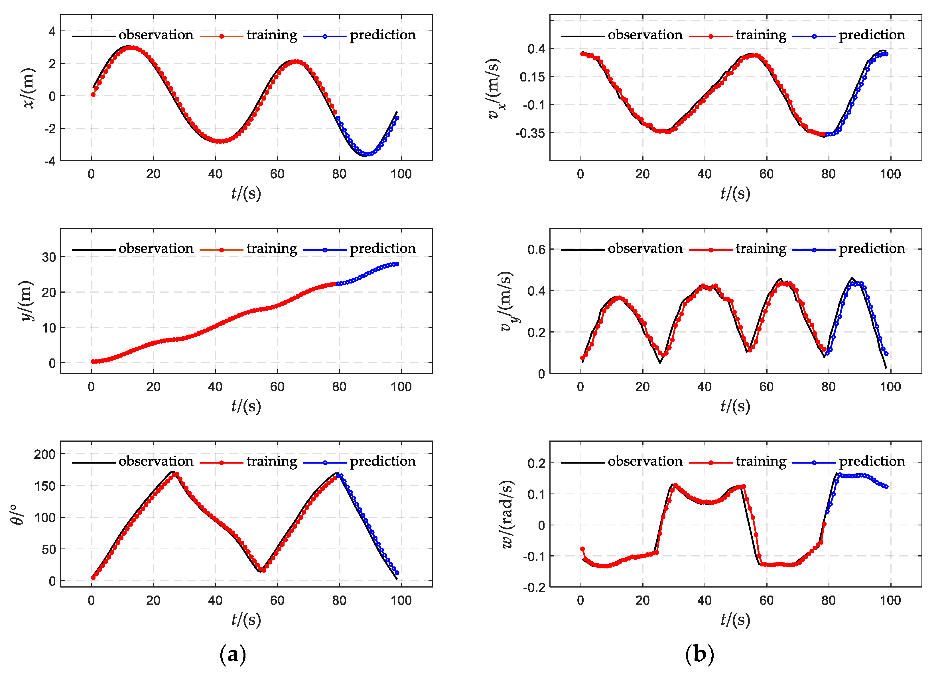
4.3. Experiment of Scaled Test Prototype

To verify the effectiveness of the black-box model, a 2:1 scaled test prototype, as displayed in Figure 13a, was developed in our laboratory, to integrate the chassis drive system, syntactic foam, control and communication systems. The crawler chassis was driven by DC 110-V brushless motors, and its precise speed regulation and position status feedback rely on hall elements and magnetic encoders. In the motor of the test prototype, a gear reducer was used to achieve a high torque instead of speed, and the maximum torque adjusted by the reducer can reach 170 Nm. During the movement process, the main controller utilised CAN bus communication to realise the setting of driving forces and the acquisition of position feedback, and sent the driving of the motors and the position information obtained by GPS and magnetic encoders to the remote monitoring terminal through the radio modem for the training and prediction of the black-box model. Furthermore, the syntactic foam used in the test prototype exhibited excellent pressure-tolerant and low water absorption, and its excellent machinability can be used for further appearance optimisation. Figure 13b displays the remote monitoring terminal used to redcord motion state, which includes a monitoring computer, radio modem, and power, to successfully realise remote control and data analysis.

Using the scaled test prototype developed in our laboratory, the comprehensive motion, on the nonlinear sand sediment near the sea, under the driving force of multi-state periodic switching, was performed to verify the generalisation and predictability of the proposed model framework. Figure 13c–e displays the various testing stages, in which the inner and outer crawler drives are set to STEP (Time, 0, 0, 0.01, 50) + STEP (Time, 25, 0, 26, 30) and STEP (Time, 0, 0, 0.01, 80) + STEP (Time, 25, 0, 26, −30), and two reciprocating cycles were set, respectively. Figure 14 displays the results of the scaled test prototype motion state $\mathit{x}(t)$ and $\mathit{q}(t)$ in 100 s, of which 70% were selected as the training datasets and 30% as the testing datasets. The results revealed the prediction data of the established PSO-SVR model were consistent with the scaled prototype testing, and the MSE and $R^2$ in

Table 4. Results of prediction accuracy of scaled test prototype.

State Quantities	x (m)	y (m)	$\mathsf{\theta }(°)$	${\mathit{v}}_{\mathit{x}} (\mathbf{m}/\mathbf{s})$	${\mathit{v}}_{\mathit{y}} (\mathbf{m}/\mathbf{s})$	w (rad/s)
MSE	0.0091	0.0032	0.0988	0.0285	0.0492	0.0115
$R^2$	0.8850	0.9960	0.9805	0.9909	0.8892	0.8351

illustrates that the model has outstanding prediction and fitting abilities.

5. Conclusions

We designed a DSLV in which tracked chassis and conventional underwater robot were combined for the scientific exploration of benthic organisms regarding the life habits of time series and distribution of sites-series. Based on the relationship between the kinematics and dynamics of the DSLV, the input and output physical quantities of the black-box motion model under the time series were clearly detailed. Next, the high-dimensional nonlinear mapping relationship between the driving force and the corresponding motion state was established using the proposed PSO-SVR model. Eventually, the black-box model framework was verified using the data of a virtual prototype simulation. To verify the effectiveness of the proposed model, we developed a 2:1 scaled test prototype in the laboratory to research the motion state of the DSLV under multi-state driving forces. The results show that the MSE and the correlation coefficient $R^2$ were close to 0 and 1, respectively, which revealed that the nonlinear motion of the DSLV can be represented by the proposed model, and the motion model can satisfy the actual requirements of scientific research. In the future, we hope that the whole system can be deployed in deep sea of 4500 m, and that the DSLV motion characteristics can be verified. Furthermore, we hope to propose a more accurate model to correct the current effect, and to define the comparison metrics to evaluate the model, such as by using Bayesian methods or PSO with local social groups to optimise the SVR. We also hope to extend the results of this research to the design of motion controllers and trajectory-tracking controllers.

References

1. Hiraoka, S.; Hirai, M.; Matsui, Y.; Makabe, A.; Minegishi, H.; Tsuda, M.; Juliarni; Rastelli, E.; Danovaro, R.; Corinaldesi, C.; et al. Microbial community and geochemical analyses of trans-trench sediments for understanding the roles of hadal environments. ISME J. 2019, 14, 740–756. [Google Scholar] [CrossRef] [PubMed] [Green Version]
2. Ishibashi, S.; Yoshida, H.; Osawa, H.; Inoue, T.; Tahara, J.; Ito, K.; Watanabe, Y.; Sawa, T.; Hyakudome, T.; Aoki, T. A ROV ABISMO for the Inspection and Sampling in the Deepest Ocean and Its Operation Support System. In Proceedings of the OCEANS 2008—MTS/IEEE Kobe Techno-Ocean Conference, Kobe, Japan, 8–11 April 2008. [Google Scholar]
3. Purser, A.; Thomsen, L.; Barnes, C.; Best, M.; Chapman, R.; Hofbauer, M.; Menzel, M.; Wagner, H. Temporal and spatial benthic data collection via an internet operated Deep Sea Crawler. Methods Oceanogr. 2013, 5, 1–18. [Google Scholar] [CrossRef]
4. McGill, P.R.; Sherman, A.D.; Hobson, B.W.; Henthorn, R.G.; Chase, A.C.; Smith, K.L. Initial Deployments of the Rover, an Autonomous Bottom-Transecting Instrument Platform for Long-Term Measurements in Deep Benthic Environments. In OCEANS 2007; IEEE: Vancouver, BC, Canada, 2007. [Google Scholar]
5. Zhang, Y.; Zhang, Q.; Yang, B.; Zhang, A. Steering Dynamic Modelling and Analysis of a Benthic Small-Scale Tracked Robot. J. Ocean. Technol. 2020, 39, 10. [Google Scholar]
6. Hongming, S.; Wei, G.; Yue, Z.; Pengfei, S.; Youbo, Z. Mechanism Design and Diving-Floating Motion Performance Analysis on the Full Ocean Depth Landing Vehicle. Robot 2020, 42, 207–214. [Google Scholar]
7. Xu, F.; Rao, Q.H.; Zhang, J.; Ma, W. Compression–shear coupling rheological constitutive model of the deep-sea sediment. Mar. Georesources Geotechnol. 2017, 36, 288–296. [Google Scholar] [CrossRef]
8. Feng, X.U.; Rao, Q.H. Turning traction force of tracked mining vehicle based on rheological property of deep-sea sediment—ScienceDirect. Trans. Nonferrous Met. Soc. China 2018, 28, 1233–1240. [Google Scholar]
9. Zhang, T.; Dai, Y.; Liu, S.J. Multi-body Dynamic Modeling and Mobility Simulation Analysis of Deep Ocean Tracked Miner. J. Mech. Eng. 2015, 51, 173–180. [Google Scholar] [CrossRef] [Green Version]
10. Inoue, T.; Shiosawa, T.; Takagi, K. Dynamic Analysis of Motion of Crawler-Type Remotely Operated Vehicles. IEEE J. Ocean. Eng. 2013, 38, 375–382. [Google Scholar] [CrossRef]
11. Sands, T. Development of Deterministic Artificial Intelligence for Unmanned Underwater Vehicles (UUV). J. Mar. Sci. Eng. 2020, 8, 578. [Google Scholar] [CrossRef]
12. Shafiei, H.M.; Binazadeh, T. Application of neural network and genetic algorithm in identification of a model of a variable mass underwater vehicle. Ocean. Eng. 2015, 96, 173–180. [Google Scholar] [CrossRef]
13. Hamzaoui, Y.E.; Rodríguez, J.; Hernández, J.; Salazar, V. Optimization of operating conditions for steam turbine using an artificial neural network inverse. Appl. Therm. Eng. 2015, 75, 648–657. [Google Scholar] [CrossRef]
14. Zhang, W.; Ding, Y.; Wang, X.; Xing, Z.; Xiang, C.; Qingxi, L. Pure Pursuit Control Method Based on SVR Inverse-model for Tractor Navigation. Trans. Chin. Soc. Agric. Mach. 2016, 47, 8. [Google Scholar]
15. Wang, X.; Zou, Z.; Ren, R. Black-Box Modeling of Ship Maneuvering Motion in 4 Degrees of Freedom Based on Support Vector Machines. Shipbuild. China 2014, 55, 147–155. [Google Scholar]
16. Man, Z.; Hahn, A.; Wen, Y.; Bolles, A. Parameter Identification of Ship Maneuvering Models Using Recursive Least Square Method Based on Support Vector Machines. TransNav Int. J. Mar. Navig. Saf. Sea Transp. 2017, 11, 23–29. [Google Scholar]
17. Koshurina, A.A.; Krasheninnikov, M.S.; Dorofeev, R.A.; Kurilsky, D.M.; Ivanov, S.A. The Analytical Review of the Condition of Unmanned Underwater Vehicles. In Proceedings of the International Conference on Advanced Manufacturing & Industrial Application, Johor Bahru, Malaysia, 20–22 September 2015. [Google Scholar]
18. Vapnik, V.N. The Nature of Statistical Learning Theory; Springer: New York, NY, USA, 1995. [Google Scholar]
19. Hazan, E.; Agarwal, A.; Kale, S. Logarithmic Regret Algorithms for Online Convex Optimization. Mach. Learn. 2007, 69, 169–192. [Google Scholar] [CrossRef]
20. Wang, Y.; Zhang, L. Properties of equation reformulation of the Karush–Kuhn–Tucker condition for nonlinear second order cone optimization problems. Math. Methods Oper. Res. 2009, 70, 195. [Google Scholar] [CrossRef]
21. Lu, Y.; Sundararajan, N. Performance evaluation of a sequential minimal radial basis function (RBF) neural network learning algorithm. IEEE Trans. Neural Netw. 1998, 9, 308–318. [Google Scholar] [PubMed]
22. Kennedy, J.; Eberhart, R. Particle Swarm Optimization. In Proceedings of the Icnn95-International Conference on Neural Networks, Perth, Australia, 27 November–1 December 1995. [Google Scholar]
23. Zhao, Y.; Liu, Z.; Zhang, Y.; Li, J.; Wang, M.; Wang, W.; Xu, J. In situ observation of contour currents in the northern South China Sea: Applications for deepwater sediment transport. Earth Planet. Sci. Lett. 2015, 430, 477–485. [Google Scholar] [CrossRef]
24. Marengo, E.; Bobba, M.; Robotti, E.; Liparota, M.C. Modeling of the Polluting Emissions from a Cement Production Plant by Partial Least-Squares, Principal Component Regression, and Artificial Neural Networks. Environ. Sci. Technol. 2006, 40, 272–280. [Google Scholar] [CrossRef] [PubMed]
25. Wu, H.; Chen, X.; Gao, Q.; He, J.S.; Liu, S.J. In-situ shearing strength and penetration resistance testing of soft seabed sediments in western mining area. J. Cent. South Univ. (Sci. Technol.) 2010, 41, 6. [Google Scholar]
26. Jiao, X.; Zhang, W.; Peng, B. RecurDyn: Optimization of Multi-Body System Simulation Technology; Tsinghua University Press: Beijing, China, 2010. [Google Scholar]
Figure 1. Schematic sketch of the demonstration mission. (Note: Sampling locations are represented by small triangles in the figure).
Jmse 10 00575 g001
Figure 2. Conceptual prototype and configure of the DSLV.
Jmse 10 00575 g002
Figure 3. Four major subsystems: (a) Chassis drive and crawling systems; (b) energy and electronic systems; (c) location and recovery systems; (d) instrument payload and communication systems.
Jmse 10 00575 g003aJmse 10 00575 g003b
Figure 4. Motion analysis of the DSLV. (a) Kinematic analysis; (b) Dynamics analysis.
Jmse 10 00575 g004
Figure 5. Structure of SVR modelling and prediction.
Jmse 10 00575 g005
Figure 6. Flowchart of PSO-SVR modelling and prediction.
Jmse 10 00575 g006
Figure 7. Pretreatment of computational fluid dynamics (CFD): (a) full-scale simplified model; (b) computational domain.
Jmse 10 00575 g007
Figure 8. Hydrodynamic resistance calculation results: (a) Velocity nephogram of DSLV at v c = 0.25 m/s; (b) Curve in hydrodynamic resistances versus velocity.
Jmse 10 00575 g008
Figure 9. Structural model and crawler system of the DSLV virtual prototype.
Jmse 10 00575 g009
Figure 10. Trajectory diagram of simulation model of DSLV. (a) Trajectory under constant driving force; (b) Trajectory under variable driving force.
Jmse 10 00575 g010
Figure 11. Results of training and prediction of constant driving force. (a) Results of training and prediction of position and yall angle; (b) Results of training and prediction of velocity and angular velocity.
Jmse 10 00575 g011
Figure 12. Results of training and prediction of variable driving force. (a) Results of training and prediction of position and yall angle; (b) Results of training and prediction of velocity and angular velocity.
Jmse 10 00575 g012
Figure 13. Scaled test prototype and the testing scenes. (a) 2:1 scaled test prototype and main components; (b) remote monitoring terminal; (c) initial motion state; (d) intermediate motion state; (e) ending motion state.
Jmse 10 00575 g013
Figure 14. Results of training and prediction of the scaled test prototype. (a) Results of traning and prediction of position and path angle; (b) Results of traning and prediction of velocity and angular velocity.
Jmse 10 00575 g014