Prediction of Aerosol Extinction Coefficient in Coastal Areas of South China Based on Attention-BiLSTM

Abstract

The aerosol extinction coefficient (AEC) characterises the attenuation of the light propagating in a turbid medium with suspended particles. Therefore, it is of great significance to carry out AEC prediction research using state-of-art neural network (NN) methods. The attention mechanism (AM) has become an indispensable part of NNs that focuses on input weight assignment. Traditional AM is used in time steps to help generate the outputs. To select important features of meteorological parameters (MP) that are helpful for forecasting, in this study, we apply AM to features instead of time steps. Then we propose a bidirectional long short-term memory (BiLSTM) NN based on AM to predict the AEC. The proposed method can remember information twice (i.e., forward and backward), which can provide more context for AEC forecasting. Finally, an in situ measured MP dataset is applied in the proposed model, which presents Maoming coastal area’s atmospheric conditions in November 2020. The experimental results show that the model proposed in this paper has higher accuracy compared with traditional NN, providing a novel solution to the AEC prediction problem for the current studies of marine aerosol.

1. Introduction

The aerosol extinction coefficient (AEC) is a measure of how strongly aerosol particles absorb and scatter light at a particular wavelength [1,2]. It is an important parameter affecting the earth–atmosphere radiative transfer system and laser light propagation [3]. AEC can also alter atmospheric visibility and thus affect the atmospheric environment [4,5,6,7]. At present, a few studies on marine aerosols are based on observed data in the United States, Europe, India, and other sea areas [8,9,10], and there is a lack of research on marine aerosols in China. It is urgently needed to carry out AEC studies in Chinese seas, especially over coastal areas. This study can provide a reference for future AEC research in China’s coastal areas.

In 2004, Piazzola et al. used MEDEX to predict the AEC in coastal zones [11], and Pen et al. developed a CAM model to predict coastal aerosol microphysical properties over China seas in 2020 [12]. However, those parameterized models may not be suitable for aerosol forecast. With the growth in available data and computing power in recent years, artificial neural networks (ANNs) provide new solutions for the prediction of atmospheric meteorological parameters [13,14,15]. ANNs are actually complex networks with a large number of simple elements connected to each other, which are highly nonlinear and can perform complex logical operations and realize nonlinear relationships [16]. Furthermore, ANNs show better prediction accuracy than statistical methods [17]. ANNs do not require much knowledge in the professional field, have low computational cost, and are widely used [18]. For instance, Pal et al. proposed a model by combining a self-organizing feature map (SOFM) and multilayer perceptron networks (MLPs) to realize a hybrid network named SOFM–MLP with better performance in atmospheric temperature prediction [19]. Zheng et al. proposed a model based on a radical basis function (RBF) NN to predict the concentration of PM2.5, which significantly increased the prediction accuracy of PM2.5 compared with classic back propagation (BP) NN [20].

However, these studies did not consider the sequence characteristics of meteorological data. Compared with traditional models, recurrent neural networks (RNNs) are generally used when input data are sequential [21,22]. However, RNNs cannot solve the gradient explosion and gradient disappearance problems caused by long-term dependencies [23]. To solve this problem, the long short-term memory (LSTM) was developed by Hochreiter and Schmidhuber as an extension of RNNs [24]. Based on LSTM, researchers have proposed many methods in time series forecasting [25]. In 2014, Cho et al. proposed the gate recurrent unit (GRU), which is performed similarly to LSTM but is computationally cheaper [26,27]. The Bidirectional-LSTM (BiLSTM) was proven to outperform undirectional ones by traversing the input data twice (i.e., (1) forward and (2) backward) [28,29]. These studies all have achieved good results in time series forecasting under specific conditions.

Attention mechanisms have become an integral part of compelling sequence modeling and transduction models in machine translation, with numerous applications in other fields as well [30,31,32,33]. In 2019, Shin et al. proposed temporal pattern attention (TPA) to select relevant time series and used it in time series forecasting. The proposed model achieves better performance in almost all of the cases than traditional RNNs and LSTMs [34].

Inspired by the above methods, this paper proposes a new model by combining an attention mechanism and BiLSTM networks to predict coastal AEC. The effectiveness of the Attention-BiLSTM network has been examined in other forecasting problems. For example, the authors in [35] used an Attention-BiLSTM in forecasting tourist arrival and achieved better accuracy than other methods considered in the same study. Liu et al. used Attention-BiLSTM to predict traffic speed, and the method was evaluated over the data of a certain area in Hangzhou [36]. The specific construction of the model proposed in this paper is as follows: (1) establishing a multi-variate temporal prediction model based on BiLSTM and (2) considering influences of different factors, adding an attention layer at the features level into the BiLSTM. The prediction results will be compared with other models.

The rest of this paper is structured as follows. Section 2 introduces the AEC prediction methodology proposed in this paper; the experimental and evaluation framework are presented in Section 3. Section 4 describes the comparison methods and experimental results. Finally, Section 5 concludes the paper.

2. Proposed Methodology of AEC Prediction

2.1. Overall Structure of the Proposed Attention-BiLSTM Method

Compared with traditional numerical weather forecasts, deep learning models are especially suitable for short-term and sudden weather forecasts and have the advantages of low cost and rapid response. AEC in marine areas is affected by various meteorological parameters and has the characteristics of large and rapid changes, and short-term changes are not periodic. The framework of the proposed method of predicting AEC in the marine area is shown in Figure 1. Timesteps is a parameter used as the memory circle in BiLSTM, which means that the input will be related to the previous $timesteps$ of the data. $features$ is the input dimension.

The detailed AEC prediction steps are described as follows:

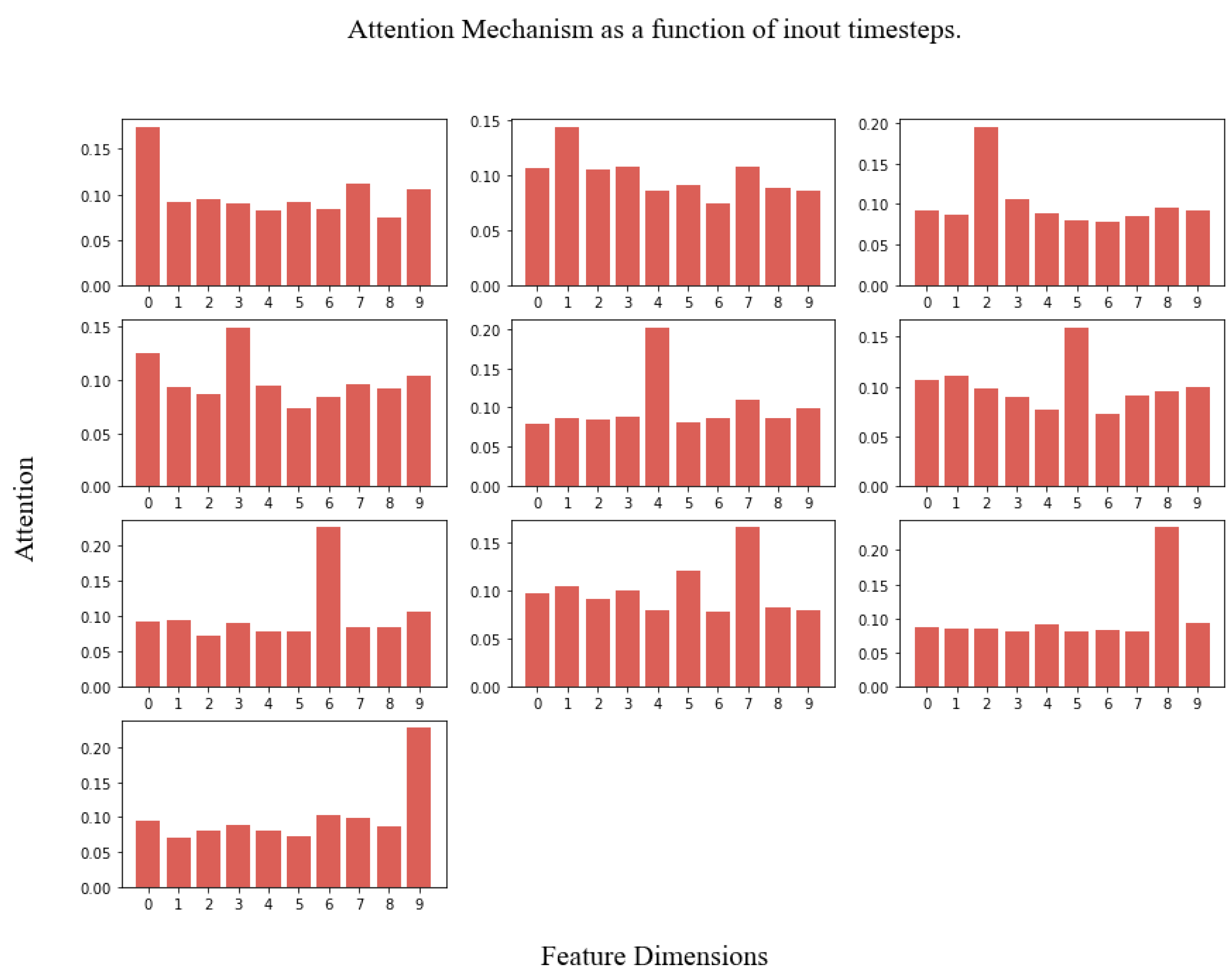
• Attention Mechanism. The traditional attention mechanism reviews the information at each previous time step and selects relevant information to help generate the output. In this paper, however, we select features dimension to find out which feature plays a key role in the prediction result:

  $$Att\_dims=Permute(timesteps,features)$$

  (1)
  After using the $permute$ operation to invert the dimensions, attention weights are multiplied by $input$ and then fed to the BiLSTM unit.
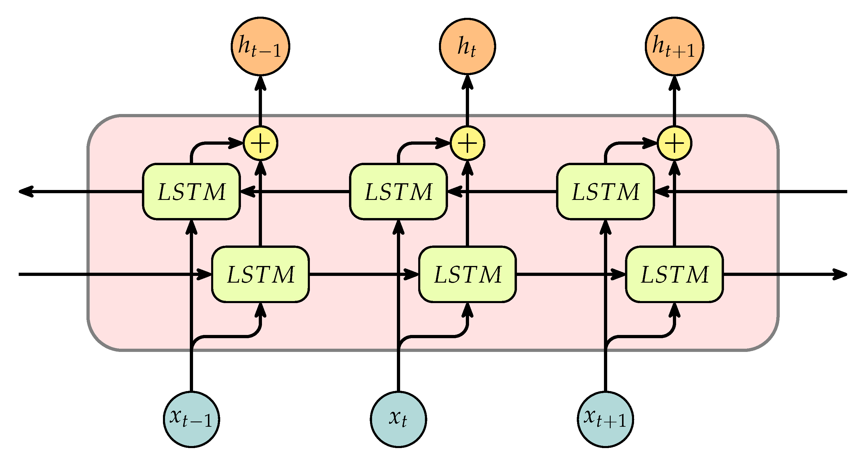
• BiLSTM unit. The BiLSTM model is used as a basic prediction model to predict AEC:

  $$X=Bidirectional\left(LSTM(lstm\_units)\right)\left(inpu{t}^{*}\right)$$

  (2)

  where $inpu{t}^{*}$ is the input multiplied by attention weights, $lstm\_units$ is hte size of the hidden layer in the BiLSTM unit. The $Bidirectional$ function is used to train data twice.
• Dense layer. A dense layer is used to convert the output of BiLSTM into a prediction result:

  $$Prediction=Activation(X·kernel+b)$$

  (3)
  Kernel is the weight matrix created by dense layer, and b is the bias vector. The activation function used in the dense layer is $linear$.

2.2. Attention Mechanism

In natural language processing (NLP), attention-based models focus mainly on changing the network architecture to improve performance on machine translate tasks. The typical attention mechanism selects information relevant to the current time step, each time step in NLP contains a single word. However, in multivariate time series forecasting, it fails to decide the importance of different variables for forecasting.

In this paper, the proposed attention mechanism basically attends to its feature vectors. The attention weights select variables that are helpful for forecasting. The modified formula is as follows:

$$a_i=softmax\left(z_i\right)={\displaystyle \frac{e^{z_i}}{{\sum }_j{e}^{z_j}}}$$

(4)

$$Attention(z,V)=\sum _i{a}_i{V}_i$$

(5)

where $z_i$ is the output of a dense layer, $a_i$ is the weight of the corresponding dimension, and V is the feature dimension. First, use the data generator to generate a 10-dimensional feature sequence, corresponding the scales of abscissa axis (i.e., 0 to 9), then select different dimensions as the objective function in turn. Figure 2 shows the effect of our proposed attention mechanism. It can be seen that the attention mechanism distributes attention weights in the corresponding dimension, indicating it can focus on important features while paying less attention to other features.

2.3. Bidirectional Long Short-Term Memory

The basic neural network only establishes weight connections between layers. To process sequence data, RNN establishes weight connections between neurons.

LSTM is specifically designed to solve the long-term dependencies problem of general RNNs. All RNNs have a chain form of repeating neural network modules. In standard RNN, this repeating module has only one tanh layer. LSTM, which is widely used, has a slightly different recurrent function:

$$h_t,w_t=F(h_{t-1},c_{t-1},x_t)$$

(6)

The repeating module of LSTM contains four interactive layers. Through three carefully designed doors, forget gate $f_t$, input gate $i_t$, and output gate $o_t$, the LSTM cell allows information to pass through selectively to protect and control the transmission of information. The forget gate $f_t$ can be written as:

$$f_t=\sigma (W_f·[h_{t-1},x_t]+b_f)$$

(7)

where $\sigma$ is the sigmoid function. $W_f$ and $b_f$ are the weights and biases, respectively. The input gate $i_t$ is similar to the forget gate $f_t$:

$$i_t=\sigma (W_i·[h_{t-1},x_t]+b_i)$$

(8)

where the weights and biases are different. The candidate memory cell ${\tilde{c}}_t$ can be represented as the combination of $h_{t-1}$ and $x_t$, and the state of cell $c_t$ can be updated by multiplying $f_t$, $c_{t-1}$, $i_t$, and ${\tilde{c}}_t$:

$${\tilde{c}}_t=tanh(W_c·[h_{t-1},x_t]+b_c)$$

(9)

$$c_t=f_t\odot c_{t-1}+i_t\odot {\tilde{c}}_t$$

(10)

After the cell gates have been updated, the output $h_t$ can be calculated by the output gate $o_t$ and cell gate $c_t$:

$$o_t=\sigma (W_o·[h_{t-1},x_t]+b_o)$$

(11)

$$h_t=o_t\odot tanh\left(c_t\right)$$

(12)

The RNN cell and LSTM cell are shown in Figure 3. In LSTM, the memory unit c can capture key information and has the ability to save it for a certain time interval. The storage period of memory unit c is longer than short-term memory h, but it is also shorter than long-term memory, so it is called long short-term memory.

BiLSTM is an extension of the LSTM model in which two LSTM cells are applied in one BiLSTM cell. Its structure is as in Figure 4. Applying LSTM twice leads to improving learning long-term dependencies and thus consequently will improve the accuracy of the model. In this work, we pass the variables related to AEC prediction into BiLSTM after attention weighting.

3. Experimental and Evaluation Framework

3.1. Data Description

The atmosphere parameters of the Maoming (APM) dataset present Maoming atmospheric data for the period of November 2020. Researchers carried out field experiments and set up experimental equipment in Maoming. After nearly a month of observation, the experiment finally collected more than 100,000 pieces of relevant data. The installation location of the instrument is marked in Figure 5. There are three main reasons why we chose this point as the observation platform:

• Marine meteorological science experiment base at Bohe, Maoming, is established and supported by the China Meteorological Administration and the Guangdong Institute of Tropical and Marine Meteorology. The station is a well-known and widely accepted experimental point for marine environment monitoring and marine climate studies.
• The terrain of the station here is flat, and it is easy to set up an observation platform; data measured and collected in this station can represent China’s typical coastal environments well;
• During that time, the weather was very good, and it was suitable for measuring coastal meteorological and atmospheric parameters.

Figure 5. Google map of Bohe observation station with a longitude of 111.32° and a latitude of 21.45°. (https://www.google.com/maps/@21.45,111.317806,8z, accessed on 8 January 2022).

Figure 5. Google map of Bohe observation station with a longitude of 111.32° and a latitude of 21.45°. (https://www.google.com/maps/@21.45,111.317806,8z, accessed on 8 January 2022).

Table 1 presents the features contained in the mentioned dataset. The data are mainly divided into three categories.

• AEC, measured by CAPS-ALB. AEC is the target value predicted in the experiment.
• General meteorological parameters, measured by WXT520. The sensor data we used in the experiment include temperature, relative humidity, and air pressure.
• Visibility, measured by SWS-100. There is no doubt that visibility is an important parameter affecting AEC. For higher accuracy, visibility is measured by SWS-100 as an independent parameter in this experiment.

Table 1. APM Properties Description.

Type	Description
Date	Observation date
AEC	Observed actual value of AEC
VIS	Observed actual value of visibility
T	Observed actual value of temperature
RH	Observed actual value of relative humidity
AP	Observed actual value of air pressure

Table 1. APM Properties Description.

Type	Description
Date	Observation date
AEC	Observed actual value of AEC
VIS	Observed actual value of visibility
T	Observed actual value of temperature
RH	Observed actual value of relative humidity
AP	Observed actual value of air pressure

3.2. Evaluation Metrics for Prediction Capacity

To fully evaluate the performance of the model, Mean Absolute Errors ($MAE$), Root Mean Squared Errors ($RMSE$), and Adjusted R-Squared ($Adj{R}^2$) were used to evaluate the prediction capacity of the proposed method from different scales:

• $MAE$ is the average value of the absolute error between the predicted value ${\tilde{y}}_i^t$ and the actual value $y_i^t$, and N represents the size of the test set. It can better reflect the actual situation of the predicted value error. The specific equation is:

  $$MAE=\frac{1}{N}\sum _{i=1}^N\left|{\tilde{y}}_i^t-y_i^t\right|$$

  (13)
• $RMSE$ is the arithmetic square root of the Mean Squared Errors ($MSE$), and $MSE$ is the expected value of the square of the difference between the estimated value of the parameter and the true value of the parameter. $RMSE$ represents the deviation of the square root between ${\tilde{y}}_i^t$ and $y_i^t$ in the total data size ratio. The smaller the value is, the better the accuracy of the prediction model to describe the experimental data. The $RMSE$ equation can be expressed by the following formula:

  $$RMSE=\sqrt{\frac{1}{N}\sum _{i=1}^N{({\tilde{y}}_t^i-y_t^i)}^2}$$

  (14)
• To analyze the prediction ability improvement of the proposed method, $Adj{R}^2$ is chosen to measures how well the predicted values fit the true values. $R^2$ is the ratio of the regression sum of squares to the total deviation of squares. The larger the ratio, the more accurate the model and the more significant the regression effect:

  $$R^2=1-\frac{\mathrm{residual}\mathrm{sum}\mathrm{of}\mathrm{squares}}{\mathrm{total}\mathrm{sum}\mathrm{of}\mathrm{squares}}=1-\frac{{\sum }_{i=1}^N{({\tilde{y}}_i-y_i)}^2}{{\sum }_{i=1}^N{({\overline{y}}_i-y_i)}^2}$$

  (15)
  $Adj{R}^2$ offsets the impact of the number of samples on R and is suitable for multiple features time series forecasting. $Adj{R}^2$ can be defined as follows:

  $$Adj{R}^2=1-\frac{(1-R^2)(N-1)}{N-P-1}$$

  (16)

  where P is the number of features. Ordinary R is suitable for describing the strength of the model’s fitting ability when describing individual features. However, as the number of samples increases, R will inevitably increase, so this paper chooses $Adj{R}^2$.
• $P_{RMSE}$ and $P_{MAE}$ represent the improvements in $RMSE$ and $MAE$, respectively. These indicators are defined as follows:

  $$P_{RMSE}=\frac{\left|RMS{E}_1-RMS{E}_2\right|}{RMS{E}_1}\times 100\%,$$

  (17)

  $$P_{MAE}=\frac{\left|MA{E}_1-MA{E}_2\right|}{MA{E}_2}\times 100\%,$$

  (18)

4. Experimental Results

4.1. Data Processing

Due to weather and power supply, the machines were not running all the time, so it is important to clean and preprocess the data. First, uninterrupted data were selected, then data were recorded every five seconds. After grouping the data in minutes, it is found that there are outliers in the data. The measured value of the instrument within a short period is NaN. The following formula was used to process the data, which makes the data smooth and more reliable:

$$data.loc\left[i\right]=\left\{\begin{array}{cc}(data.loc[i-1]+data.loc[i-2\left]\right)/2,\hfill & \mathrm{if}data.loc.\left[i\right]<(data.loc[i-1]+data.loc[i+1\left]\right)/3\hfill \\ data.loc\left[i\right],\hfill & \mathrm{if}data.loc.\left[i\right]\ge (data.loc[i-1]+data.loc[i+1\left]\right)/3\hfill \end{array}\right.$$

(19)

Among them, $lo{c}_i$ is the current data, $lo{c}_{i-1}$ and $lo{c}_{i-2}$ are the data one time step and two time steps before, and $lo{c}_{i+1}$ is the data after one time step. The processed data are shown as Figure 6.

Feature scaling is an important content in data preprocessing. There are two reasons why we need feature scaling in this experiment:

• Different features have different scales, in order to eliminate the influence of the unit and scale differences between features and treat each dimension feature equally, it is necessary to normalize the features.
• For the loss function of the model, gradient descent converges faster after feature scaling.

The scaling method used in this paper is the min–max scaler, which is very sensitive to outliers because outliers affect the max or min value, so this method is only suitable for the case where the data are distributed in a range. The Min–max scaler can be written as:

$$x^{*}={\displaystyle \frac{x-min\left(x\right)}{max\left(x\right)-min\left(x\right)}}$$

(20)

where x is the current data, $min\left(x\right)$ is the minimum, $max\left(x\right)$ is the maximum, and $x^{*}$ is the normalized data.

The Figure 7 show that temperature and relative humidity have obvious periodicity. The temperature is highest around noon and lowest around midnight. The relative humidity is lowest around noon and highest at midnight.

4.2. Comparison Methods

To verify the predictive capacity of the proposed prediction method fairly, we compared it with six comparison methods: Multilayer Perceptron (MLP), RNN, LSTM, GRU, BiLSTM, and BiLSTM-Attention. RNN, LSTM, and BiLSTM have been introduced in Section 2. The others are as follows:

• MLP method
  MLP is a class of feed-forward (FF) NNs. MLP utilizes a supervised learning technique called back-propagation for training. Its multiple layers and non-linear activation distinguish MLP from a linear perceptron. It can distinguish data that are not linearly separable.
• GRU method
  GRU is a variant of the LSTM neural network [37]. It combines the forget and output gates in the LSTM into a new gate called the update gate to obtain fewer parameters and faster training speeds. GRU has been shown to exhibit better performance on certain smaller and less frequent datasets.
• BiLSTM-Attention method
  This method is similar to the proposed method in this paper. The difference is that this method puts attention after BiLSTM.

4.3. Results Analysis and Discussion

To improve the reliability of the experimental results, we chose two datasets to verify the ability of the proposed method (dataset A: 19 November 2020 6:53 to 14:57; dataset B: 20 November 2020 0:05 to 18:00). After data preparation and selection of comparison methods, we draw two main conclusions from the experimental results:

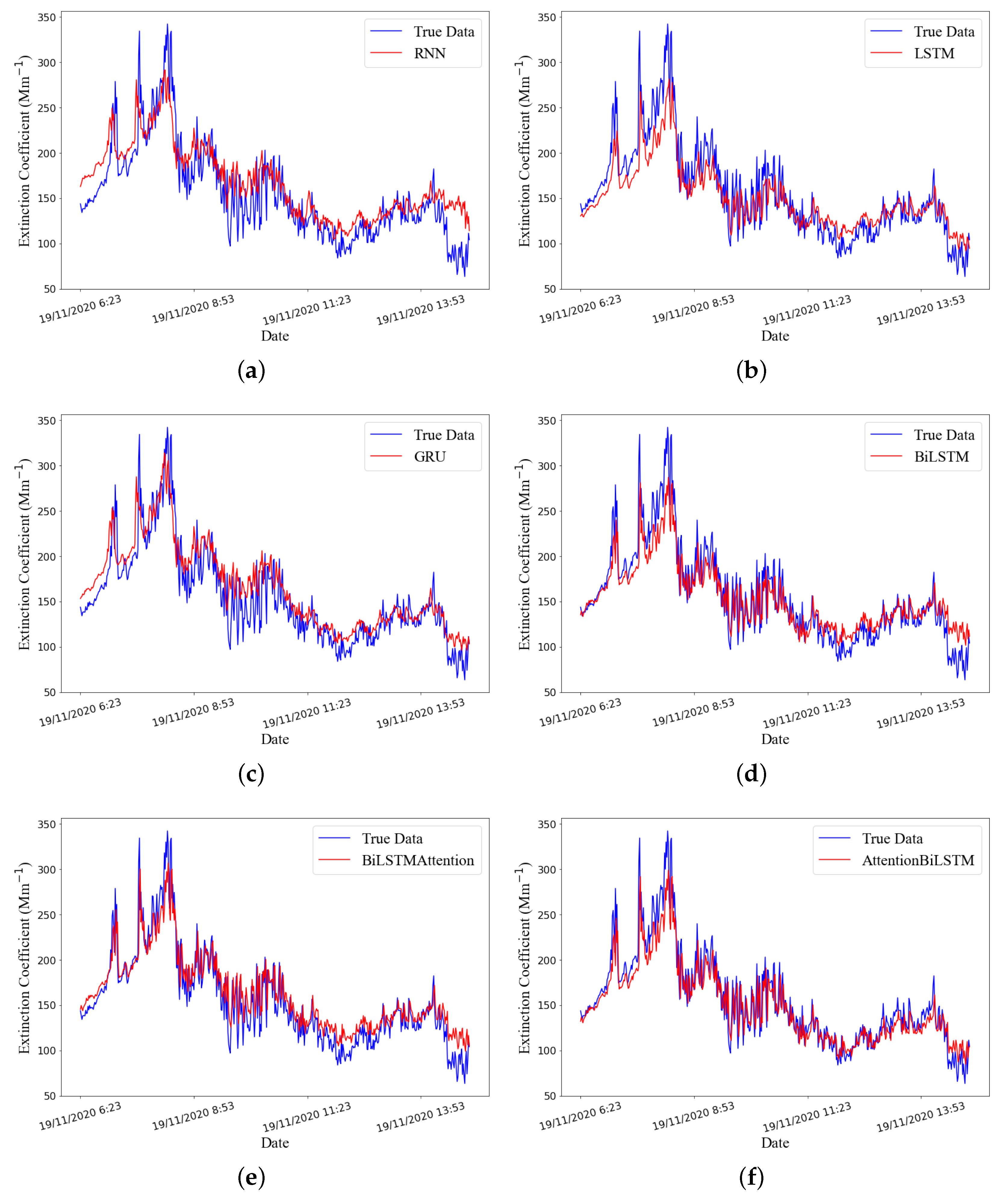
• Models based on LSTM obtain better performance than the traditional RNN model.
  As

  Table 2. Percentage Improvement of Methods in Comparisons with MLP (dataset A).

  Prediction Approaches	${\mathit{P}}_{\mathit{RMSE}}$	${\mathit{P}}_{\mathit{MAE}}$	${\mathit{AdjR}}^2$
  RNN	33.1%	36.8%	0.679
  LSTM	41.8%	45.0%	0.758
  GRU	47.4%	48.8%	0.804
  BiLSTM	50.0%	51.5%	0.821
  BiLSTM-Attention	51.0%	55.0%	0.829
  Proposed Method	52.8%	56.6%	0.84

  and

  Table 3. Percentage Improvement of Methods in Comparisons with MLP (dataset B).

  Prediction Approaches	${\mathit{P}}_{\mathit{RMSE}}$	${\mathit{P}}_{\mathit{MAE}}$	${\mathit{AdjR}}^2$
  RNN	21.1%	16.4%	0.727
  LSTM	30.4%	28.0%	0.788
  GRU	33.0%	31.4%	0.808
  BiLSTM	36.3%	34.6%	0.822
  BiLSTM-Attention	46.2%	44.9%	0.873
  Proposed Method	51.3%	51.4%	0.896

  show that for the AEC prediction in the Maoming area, the LSTM and LSTM variants have higher prediction accuracy than RNN. For instance, compared with the MLP, other methods’ percentage improvements in $RMSE$ were $33.1\%$, $41.8\%$, $47.4\%$, $50.0\%$, $51.0\%$, and $52.8\%$, respectively, in dataset A, while they were $21.1\%$, $30.4\%$, $33.0\%$, $36.3\%$, $46.2\%$, and $51.3\%$, respectively, in dataset B; the percentage improvements in $MAE$ were $36.8\%$, $45.0\%$, $48.8\%$, $51.5\%$, $55.0\%$, and $56.6\%$, respectively, in dataset A, while they were $16.4\%$, $28.0\%$, $31.4\%$, $34.6\%$, $44.9\%$, and $51.4\%$, respectively, in dataset B.
  Figure 8 shows the estimated prediction error results of different AEC prediction methods in APM. According to this figure, some positive findings could be obtained: (1) LSTM methods have higher prediction accuracy than traditional methods in AEC prediction; (2) compared with normal LSTM methods, the forecasting capacities of BiLSTM approaches is superior; and (3) the attention mechanism can slightly improve the accuracy of prediction.
• The BiLSTM model based on the attention mechanism achieves a better prediction effect than other methods.
  Figure 9 shows different methods’ performances in a Taylor diagram, which is often used to evaluate the accuracy of models. The scatter in the Taylor diagram represents the model; the radial distance from the dot represents the ratio of the standard deviation of the model to the observation, indicating the model’s ability to simulate the center amplitude. The closer the standard deviation is to one, the better the simulation ability; $RMSE$ is a measure of the distance between the model and the observation, represented in the figure as a dotted green semicircle with point A as the center; the correlation coefficient is determined by the azimuth position of the model. When the model prediction result is more consistent with the observed value, the closer the model point is to the observation point in the x-axis; thus, the model has a high correlation with the observation. This figure shows that the method proposed in this paper obtains the best performance in AEC prediction than other traditional NN methods.

As shown in Figure 10 and Figure 11, all LSTMs can predict the trend of AEC well. We can also obtain two main points: (1) Despite its high accuracy, GRU is less capable of capturing data changes than LSTM; (2) compared with BiLSTM-Attention, the proposed prediction method can better capture the data changes while obtaining the best prediction effect.

5. Concluding Remarks

In this paper, we reviewed recent published works that involve the use of NN algorithms for time series forecasting. The main NN algorithms, including ANNs, RNNs, LSTMs, Attention-based models, and their applications, were introduced first. After a discussion of the reviewed studies, a model used for AEC prediction was proposed. It can be divided into two main parts: (a) the Attention Mechanism and (b) the BiLSTM. The proposed model, namely, Attention-BiLSTM, combines the attention mechanism’s weight-selection ability with BiLSTM’s ability to predict process sequence features to predict AEC.

The experimental data were collected from Maoming, China, in November 2020. Then we preprocessed the data to make them smooth. This paper reported the results of the experiment, through which the performance and accuracy, as well as the behavioral training of MLP, RNN, LSTM, BiLSTM, BiLSTM-Attention, and Attention-BiLSTM models, were analyzed and compared. The model proposed in this paper has improved accuracy by 23.7% compared with the classic RNN. Compared with other different LSTM variants, the accuracy is improved and the changes in data trends can be captured accurately.

Although many new models have been developed for time series forecasting those years, some limitations still exist and may impose non-negligible effect on the AEC forecasting. Firstly, in the process of collecting experimental data, the missing data phenomenon occurs from time to time. Secondly, current research mostly focuses on short-term forecasts, and long-sequence forecasts are more desirable. Therefore, our next research can be expanded in the following ways:

• Different meteorological parameters need to be added as features in the future. According to attention mechanism theory, our method will automatically adjusts the weights of different features.
• More geographic locations should be selected for prediction, which will make experimental results more convincing.
• Long-sequence time-series forecasting (LSTF) must be considered. In practical application problems, we need to forecast long time series. Our next work, we will focus on improving the forecast time and making the research more practical while ensuring the forecast accuracy.

References

1. Ramanathan, V.; Crutzen, P.J.; Kiehl, J.; Rosenfeld, D. Aerosols, climate, and the hydrological cycle. Science 2001, 294, 2119–2124. [Google Scholar] [CrossRef] [PubMed] [Green Version]
2. Lyamani, H.; Olmo, F.; Alados-Arboledas, L. Light scattering and absorption properties of aerosol particles in the urban environment of Granada, Spain. Atmos. Environ. 2008, 42, 2630–2642. [Google Scholar] [CrossRef]
3. Griggs, M. Measurements of atmospheric aerosol optical thickness over water using ERTS-1 data. J. Air Pollut. Control Assoc. 1975, 25, 622–626. [Google Scholar] [CrossRef] [PubMed] [Green Version]
4. Remer, L.A.; Kaufman, Y.J.; Holben, B.N. Interannual variation of ambient aerosol characteristics on the east coast of the United States. J. Geophys. Res. Atmos. 1999, 104, 2223–2231. [Google Scholar] [CrossRef]
5. Kanakidou, M.; Seinfeld, J.; Pandis, S.; Barnes, I.; Dentener, F.J.; Facchini, M.C.; Dingenen, R.V.; Ervens, B.; Nenes, A.; Nielsen, C.; et al. Organic aerosol and global climate modelling: A review. Atmos. Chem. Phys. 2005, 5, 1053–1123. [Google Scholar] [CrossRef] [Green Version]
6. Kaufman, Y.J.; Tanré, D.; Boucher, O. A satellite view of aerosols in the climate system. Nature 2002, 419, 215–223. [Google Scholar] [CrossRef]
7. Chatterjee, A.; Michalak, A.M.; Kahn, R.A.; Paradise, S.R.; Braverman, A.J.; Miller, C.E. A geostatistical data fusion technique for merging remote sensing and ground-based observations of aerosol optical thickness. J. Geophys. Res. Atmos. 2010, 115. [Google Scholar] [CrossRef] [Green Version]
8. Gathman, S.G. Optical properties of the marine aerosol as predicted by the Navy aerosol model. Opt. Eng. 1983, 22, 220157. [Google Scholar] [CrossRef]
9. Vignati, E.; De Leeuw, G.; Berkowicz, R. Modeling coastal aerosol transport and effects of surf-produced aerosols on processes in the marine atmospheric boundary layer. J. Geophys. Res. Atmos. 2001, 106, 20225–20238. [Google Scholar] [CrossRef] [Green Version]
10. Tedeschi, G.; Piazzola, J. Development of a 2D marine aerosol transport model: Application to the influence of thermal stability in the marine atmospheric boundary layer. Atmos. Res. 2011, 101, 469–479. [Google Scholar] [CrossRef]
11. Piazzola, J.J.; Kaloshin, G.; De Leeuw, G.; van Eijk, A.M. Aerosol extinction in coastal zones. In Proceedings of the Optics in Atmospheric Propagation and Adaptive Systems VII; International Society for Optics and Photonics: Bellingham, WA, USA, 2004; Volume 5572, pp. 94–100. [Google Scholar]
12. Pan, Y.; Cui, S.; Rao, R. A model for predicting coastal aerosol size distributions in Chinese seas. Earth Space Sci. 2020, 7, e2020EA001136. [Google Scholar] [CrossRef]
13. Wang, S.C. Artificial neural network. In Interdisciplinary Computing in Java Programming; Springer: Berlin/Heidelberg, Germany, 2003; pp. 81–100. [Google Scholar]
14. Gupta, N. Artificial neural network. Netw. Complex Syst. 2013, 3, 24–28. [Google Scholar]
15. Abiodun, O.I.; Jantan, A.; Omolara, A.E.; Dada, K.V.; Mohamed, N.A.; Arshad, H. State-of-the-art in artificial neural network applications: A survey. Heliyon 2018, 4, e00938. [Google Scholar] [CrossRef] [Green Version]
16. De Gooijer, J.G.; Hyndman, R.J. 25 years of time series forecasting. Int. J. Forecast. 2006, 22, 443–473. [Google Scholar] [CrossRef] [Green Version]
17. Zhang, G.; Patuwo, B.E.; Hu, M.Y. Forecasting with artificial neural networks: The state of the art. Int. J. Forecast. 1998, 14, 35–62. [Google Scholar] [CrossRef]
18. Yegnanarayana, B. Artificial Neural Networks; PHI Learning Pvt. Ltd.: Delhi, India, 2009. [Google Scholar]
19. Pal, N.R.; Pal, S.; Das, J.; Majumdar, K. SOFM-MLP: A hybrid neural network for atmospheric temperature prediction. IEEE Trans. Geosci. Remote Sens. 2003, 41, 2783–2791. [Google Scholar] [CrossRef]
20. Haiming, Z.; Xiaoxiao, S. Study on prediction of atmospheric PM2.5 based on RBF neural network. In Proceedings of the 2013 Fourth International Conference on Digital Manufacturing & Automation, Qindao, China, 29–30 June 2013; pp. 1287–1289. [Google Scholar]
21. Connor, J.T.; Martin, R.D.; Atlas, L.E. Recurrent neural networks and robust time series prediction. IEEE Trans. Neural Netw. 1994, 5, 240–254. [Google Scholar] [CrossRef] [Green Version]
22. Hüsken, M.; Stagge, P. Recurrent neural networks for time series classification. Neurocomputing 2003, 50, 223–235. [Google Scholar] [CrossRef]
23. Pascanu, R.; Mikolov, T.; Bengio, Y. On the difficulty of training recurrent neural networks. In Proceedings of the International Conference on Machine Learning PMLR, Atlanta, GA, USA, 17–19 June 2013; pp. 1310–1318. [Google Scholar]
24. Hochreiter, S.; Schmidhuber, J. Long short-term memory. Neural Comput. 1997, 9, 1735–1780. [Google Scholar] [CrossRef]
25. Greff, K.; Srivastava, R.K.; Koutník, J.; Steunebrink, B.R.; Schmidhuber, J. LSTM: A search space odyssey. IEEE Trans. Neural Netw. Learn. Syst. 2016, 28, 2222–2232. [Google Scholar] [CrossRef] [Green Version]
26. Cho, K.; Van Merriënboer, B.; Bahdanau, D.; Bengio, Y. On the properties of neural machine translation: Encoder-decoder approaches. arXiv 2014, arXiv:1409.1259. [Google Scholar]
27. Chung, J.; Gulcehre, C.; Cho, K.; Bengio, Y. Empirical evaluation of gated recurrent neural networks on sequence modeling. arXiv 2014, arXiv:1412.3555. [Google Scholar]
28. Graves, A.; Schmidhuber, J. Framewise phoneme classification with bidirectional LSTM and other neural network architectures. Neural Netw. 2005, 18, 602–610. [Google Scholar] [CrossRef] [PubMed]
29. Siami-Namini, S.; Tavakoli, N.; Namin, A.S. The performance of LSTM and BiLSTM in forecasting time series. In Proceedings of the 2019 IEEE International Conference on Big Data (Big Data), Los Angeles, CA, USA, 9–12 December 2019; pp. 3285–3292. [Google Scholar]
30. Bahdanau, D.; Cho, K.; Bengio, Y. Neural machine translation by jointly learning to align and translate. arXiv 2014, arXiv:1409.0473. [Google Scholar]
31. Luong, M.T.; Pham, H.; Manning, C.D. Effective approaches to attention-based neural machine translation. arXiv 2015, arXiv:1508.04025. [Google Scholar]
32. Kim, Y.; Denton, C.; Hoang, L.; Rush, A.M. Structured attention networks. arXiv 2017, arXiv:1702.00887. [Google Scholar]
33. Vaswani, A.; Shazeer, N.; Parmar, N.; Uszkoreit, J.; Jones, L.; Gomez, A.N.; Kaiser, Ł.; Polosukhin, I. Attention is all you need. In Proceedings of the Advances in Neural Information Processing Systems, Long Beach, CA, USA, 4–9 December 2017; pp. 5998–6008. [Google Scholar]
34. Shih, S.Y.; Sun, F.K.; Lee, H.Y. Temporal pattern attention for multivariate time series forecasting. Mach. Learn. 2019, 108, 1421–1441. [Google Scholar] [CrossRef] [Green Version]
35. Adil, M.; Wu, J.Z.; Chakrabortty, R.K.; Alahmadi, A.; Ansari, M.F.; Ryan, M.J. Attention-Based STL-BiLSTM Network to Forecast Tourist Arrival. Processes 2021, 9, 1759. [Google Scholar] [CrossRef]
36. Liu, D.; Tang, L.; Shen, G.; Han, X. Traffic speed prediction: An attention-based method. Sensors 2019, 19, 3836. [Google Scholar] [CrossRef] [Green Version]
37. Chen, J.; Jing, H.; Chang, Y.; Liu, Q. Gated recurrent unit based recurrent neural network for remaining useful life prediction of nonlinear deterioration process. Reliab. Eng. Syst. Saf. 2019, 185, 372–382. [Google Scholar] [CrossRef]
Figure 1. The framework of the method proposed in this paper.
Jmse 10 00545 g001
Figure 2. Distribution of attention weights after introducing the attention mechanism.
Jmse 10 00545 g002
Figure 3. Diagram of structures of (a) RNN and (b) LSTM cells.
Jmse 10 00545 g003
Figure 4. Workflow for simple BiLSTM model.
Jmse 10 00545 g004
Figure 6. Coastal meteorological parameters of the Maoming area in November 2020.
Jmse 10 00545 g006
Figure 7. Boxplot of different features: (a) Hourly Air Pressure Statistics, (b) Hourly Temperature Statistics, (c) Hourly Relative Humidity Statistics, and (d) Hourly Visibility Statistics.
Jmse 10 00545 g007
Figure 8. Error estimation result of AEC prediction methods in (a) dataset A and (b) dataset B.
Jmse 10 00545 g008
Figure 9. Taylor diagram of different models in (a) dataset A and (b) dataset B.
Jmse 10 00545 g009
Figure 10. The performance of prediction in dataset A by using (a) RNN, (b) LSTM, (c) GRU, (d) BiLSTM, (e) BiLSTMAttention, and (f) Proposed Method.
Jmse 10 00545 g010
Figure 11. The performance of prediction in dataset B by using (a) RNN, (b) LSTM, (c) GRU, (d) BiLSTM, (e) BiLSTMAttention, and (f) Proposed Method.
Jmse 10 00545 g011