
Real-Time Ship Tracking under Challenges of Scale Variation and Different Visibility Weather Conditions


Abstract
:1. Introduction
2. Methodology
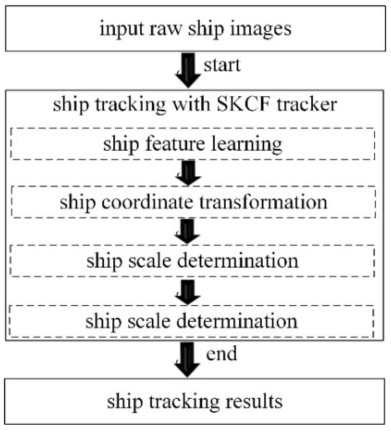
2.1. Framework Overview
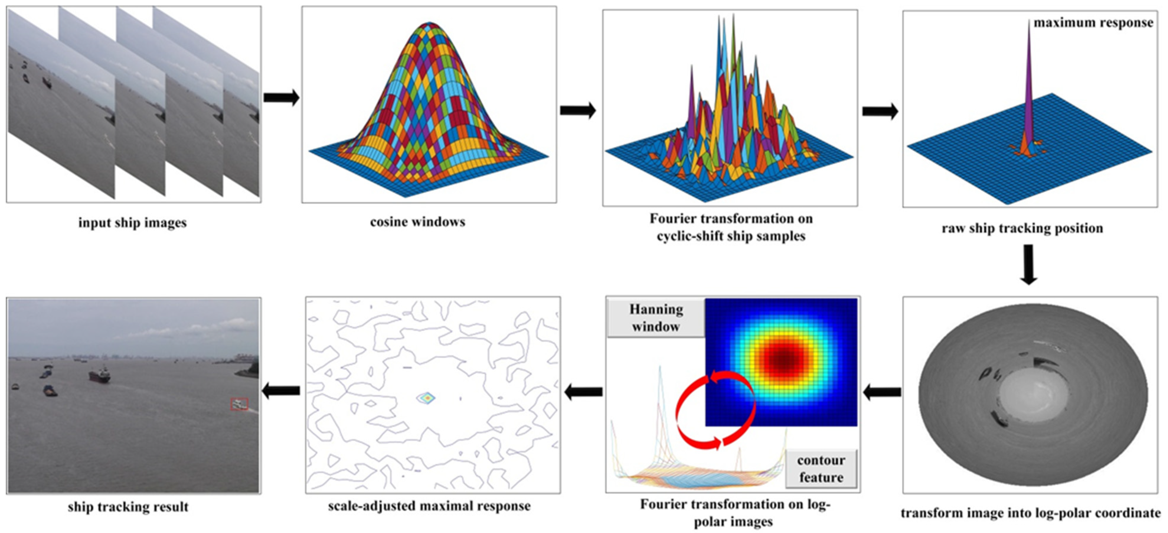
2.2. Ship Tracking with KCF
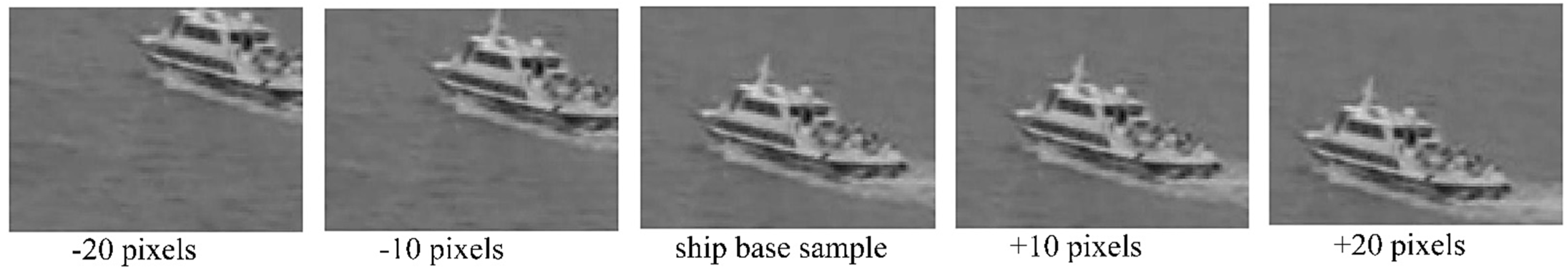
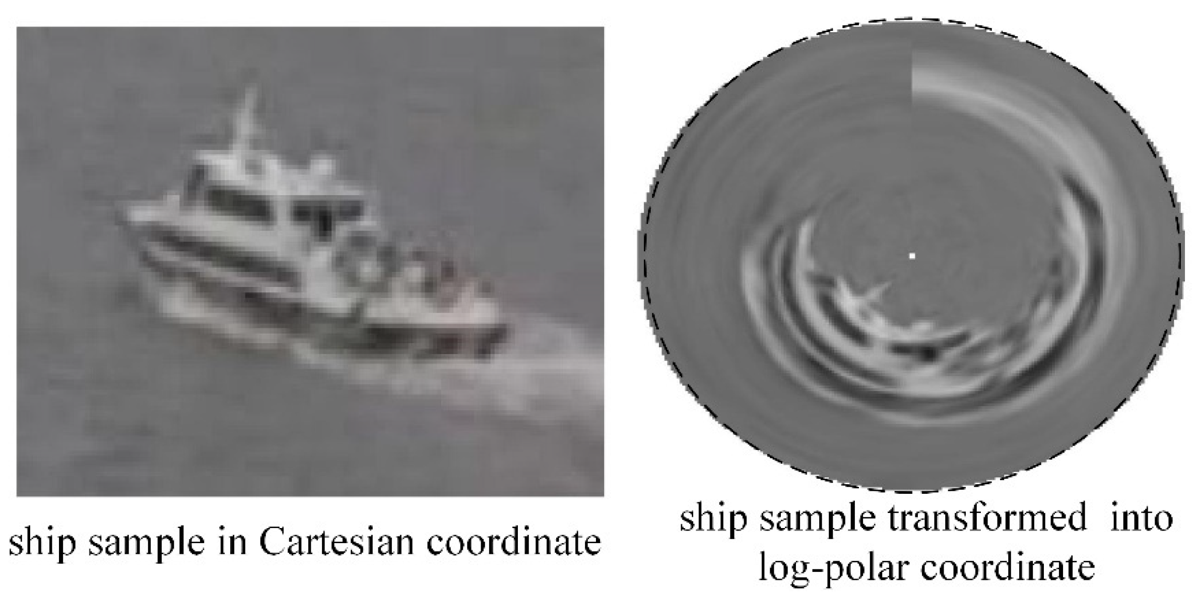
2.3. Ship Scale Refinement
| Algorithm 1 The proposed SKCF ship tracker |
| Input: Ship images and ship position in the first frame. |
| Output: Estimated ship tracking position in current frame; ifthe initial ship framethen 1. Performs parameter initialization; 2. Extracts pre-trained ship patterns and labels; 3. Trains the ship tracker in Fourier domain; else 4. Extracts ship features from the previous image; 5. Transforms the ship image into Fourier domain; 6. Obtains maximal response and obtains raw ship position; 7. Transforms the ship (i.e., raw tracking result) and sample into the log-polar coordinate system; 8. Obtains maximal response in Fourier domain; 9. Determines ship scale factor; end |
3. Experiments
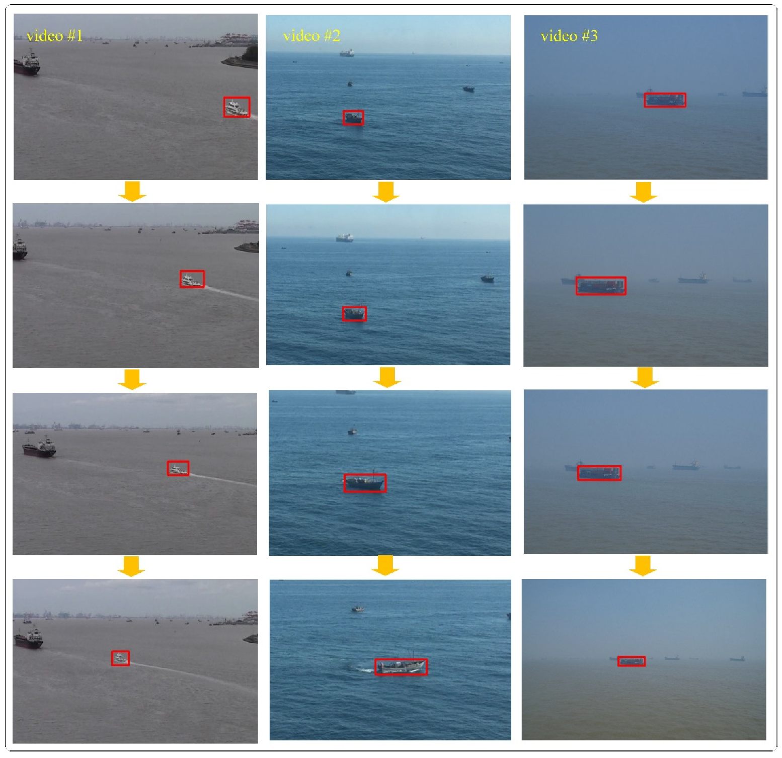
3.1. Data
3.2. Tracking Performance Measurements
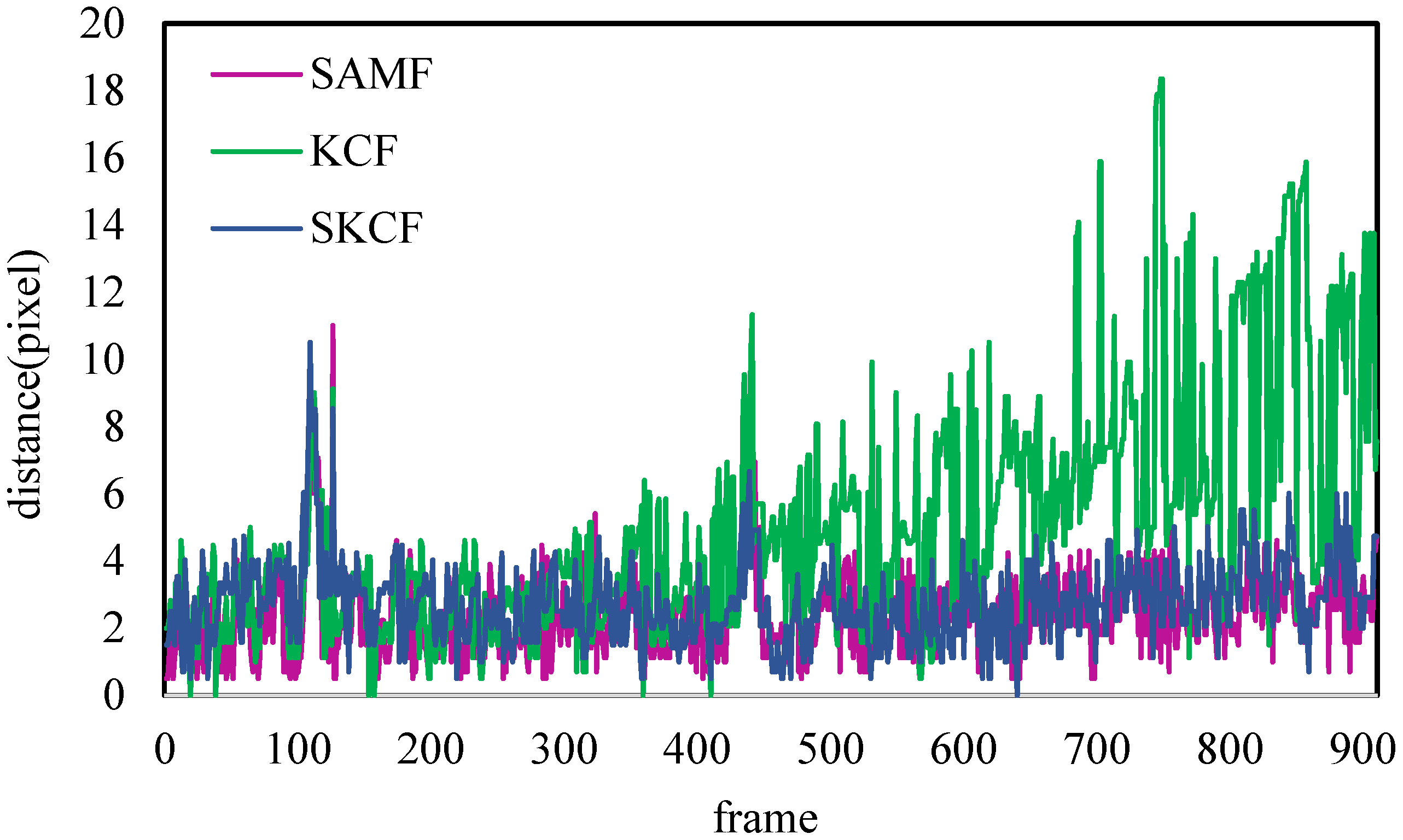
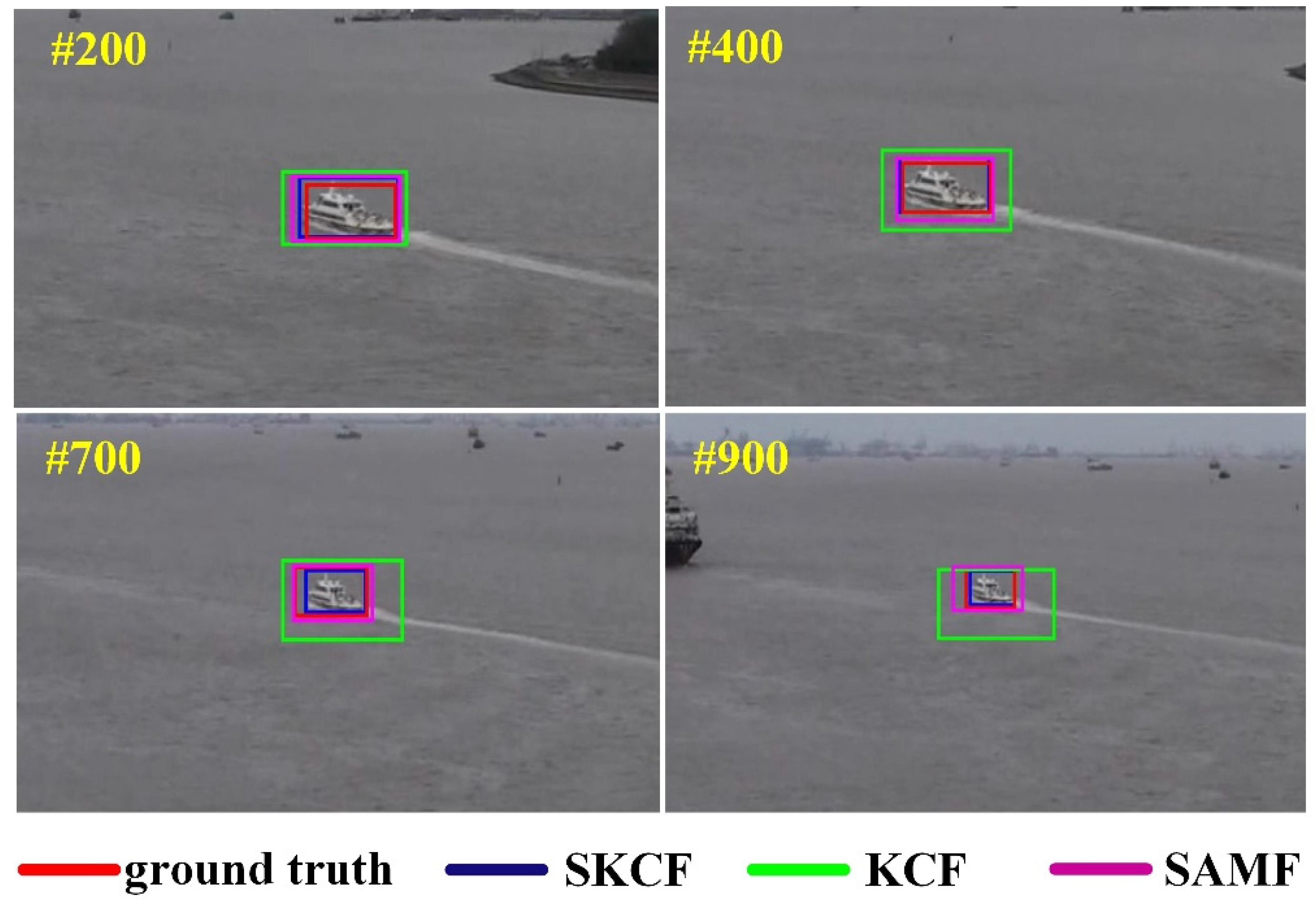
3.3. Ship Tracking Results on Video #1
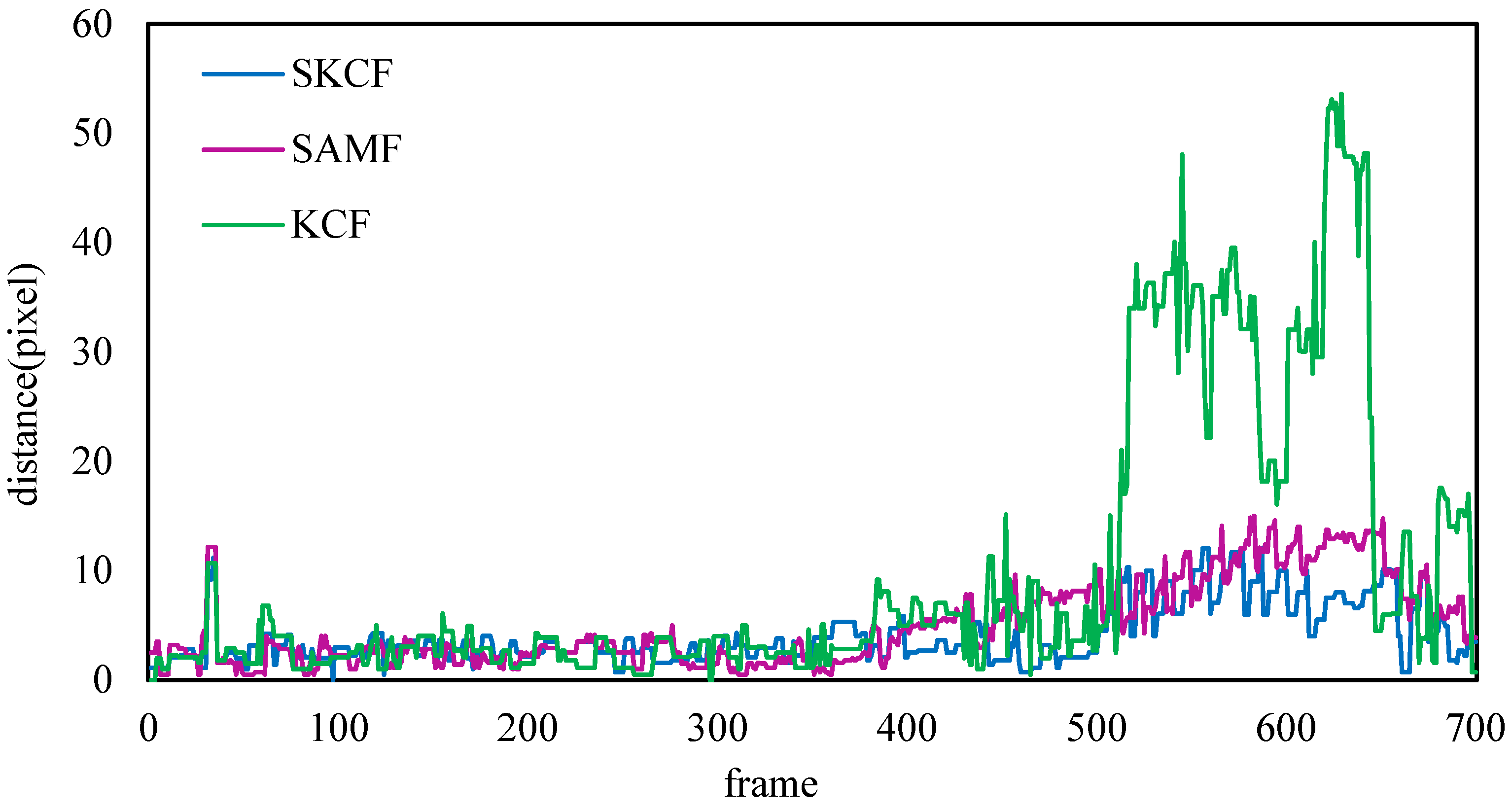
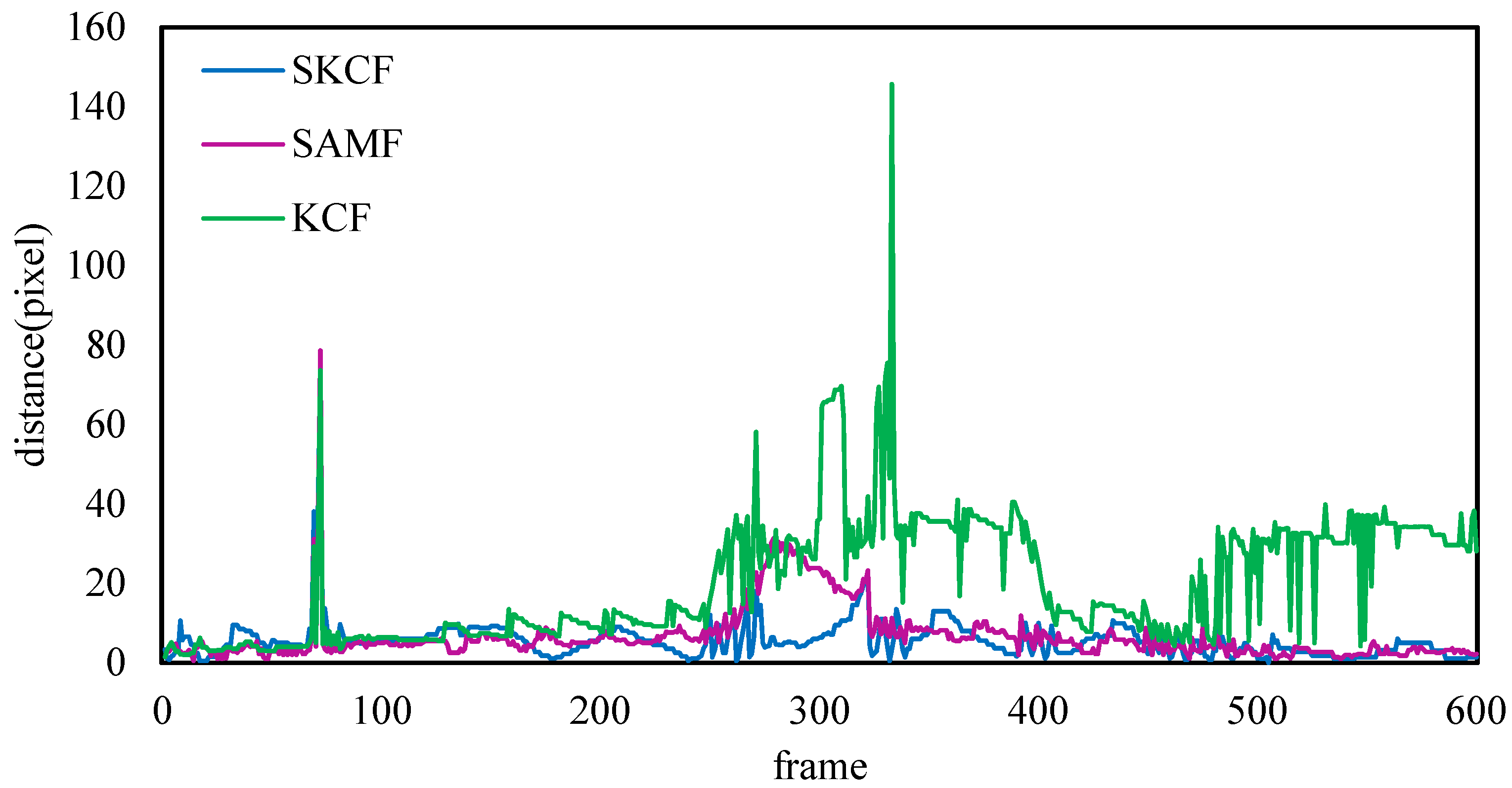
3.4. Ship Tracking Results on Videos #2 and #3
4. Conclusions
Author Contributions
Funding
Institutional Review Board Statement
Informed Consent Statement
Data Availability Statement
Conflicts of Interest
References
- Yan, X.; Wang, K.; Yuan, Y.; Jiang, X.; Negenborn, R.R. Energy-efficient shipping: An application of big data analysis for optimizing engine speed of inland ships considering multiple environmental factors. Ocean Eng. 2018, 169, 457–468. [Google Scholar] [CrossRef]
- Zhu, M.; Sun, W.; Hahn, A.; Wen, Y.; Xiao, C.; Tao, W. Adaptive modeling of maritime autonomous surface ships with uncertainty using a weighted LS-SVR robust to outliers. Ocean Eng. 2020, 200, 107053. [Google Scholar] [CrossRef]
- Wu, B.; Cheng, T.; Yip, T.L.; Wang, Y. Fuzzy logic based dynamic decision-making system for intelligent navigation strategy within inland traffic separation schemes. Ocean Eng. 2020, 197, 106909. [Google Scholar] [CrossRef]
- Zhou, F.; Pan, S.; Jiang, J. Verification of AIS Data by using Video Images taken by a UAV. J. Navig. 2019, 72, 1345–1358. [Google Scholar] [CrossRef]
- Jiang, M.; Shen, J.; Kong, J.; Huo, H. Regularization Learning of Correlation Filter for Robust Visual Tracking. IET Image Process. 2018, 12, 1586–1594. [Google Scholar] [CrossRef]
- Ma, W.; Hao, S.; Ma, D.; Wang, D.; Jin, S.; Qu, F. Scheduling decision model of liner shipping considering emission control areas regulations. Appl. Ocean Res. 2021, 106, 102416. [Google Scholar] [CrossRef]
- Zhang, W.; Zou, Z.; Goerlandt, F.; Qi, Y.; Kujala, P. A multi-ship following model for icebreaker convoy operations in ice-covered waters. Ocean Eng. 2019, 180, 238–253. [Google Scholar] [CrossRef]
- Ma, D.; Ma, W.; Jin, S.; Ma, X. Method for simultaneously optimizing ship route and speed with emission control areas. Ocean Eng. 2020, 202, 107170. [Google Scholar] [CrossRef]
- Liu, R.W.; Liang, M.; Nie, J.; Lim, W.Y.B.; Zhang, Y.; Guizani, M. Deep Learning-Powered Vessel Trajectory Prediction for Improving Smart Traffic Services in Maritime Internet of Things. IEEE Trans. Netw. Sci. Eng. 2022. Early access. [Google Scholar] [CrossRef]
- Ma, D.; Ma, W.; Hao, S.; Jin, S.; Qu, F. Ship’s response to low-sulfur regulations: From the perspective of route, speed and refueling strategy. Comput. Ind. Eng. 2021, 155, 107140. [Google Scholar] [CrossRef]
- Fang, Z.; Yu, H.; Ke, R.; Shaw, S.-L.; Peng, G. Automatic Identification System-Based Approach for Assessing the Near-Miss Collision Risk Dynamics of Ships in Ports. IEEE Trans. Intell. Transp. Syst. 2019, 20, 534–543. [Google Scholar] [CrossRef]
- Chen, Z.; Xue, J.; Wu, C.; Qin, L.; Liu, L.; Cheng, X. Classification of vessel motion pattern in inland waterways based on Automatic Identification System. Ocean Eng. 2018, 161, 69–76. [Google Scholar] [CrossRef]
- Yang, D.; Wu, L.; Wang, S.; Jia, H.; Li, K.X. How big data enriches maritime research–a critical review of Automatic Identification System (AIS) data applications. Transp. Rev. 2019, 39, 755–773. [Google Scholar] [CrossRef]
- Hörteborn, A.; Ringsberg, J.W.; Svanberg, M.; Holm, H. A Revisit of the Definition of the Ship Domain based on AIS Analysis. J. Navig. 2019, 72, 777–794. [Google Scholar] [CrossRef]
- Ma, W.; Lu, T.; Ma, D.; Wang, D.; Qu, F. Ship route and speed multi-objective optimization considering weather conditions and emission control area regulations. Marit. Policy Manag. 2020, 48, 1053–1068. [Google Scholar] [CrossRef]
- Zhao, L.; Shi, G. Maritime Anomaly Detection using Density-based Clustering and Recurrent Neural Network. J. Navig. 2019, 72, 894–916. [Google Scholar] [CrossRef]
- Wu, B.; Yip, T.L.; Yan, X.; Soares, C.G. Review of techniques and challenges of human and organizational factors analysis in maritime transportation. Reliab. Eng. Syst. Saf. 2021, 219, 108249. [Google Scholar] [CrossRef]
- Prasad, D.K.; Dong, H.; Rajan, D.; Quek, C. Are Object Detection Assessment Criteria Ready for Maritime Computer Vision? IEEE Trans. Intell. Transp. Syst. 2020, 21, 5295–5304. [Google Scholar] [CrossRef] [Green Version]
- Prasad, D.K.; Prasath, C.K.; Rajan, D.; Rachmawati, L.; Rajabally, E.; Quek, C. Object Detection in a Maritime Environment: Performance Evaluation of Background Subtraction Methods. IEEE Trans. Intell. Transp. Syst. 2018, 20, 1787–1802. [Google Scholar] [CrossRef]
- Kong, J.; Wang, B.; Jiang, M. Robust part-based visual tracking via adaptive collaborative modelling. IET Image Process. 2019, 13, 1648–1657. [Google Scholar] [CrossRef]
- Chen, X.; Qi, L.; Yang, Y.; Luo, Q.; Postolache, O.; Tang, J.; Wu, H. Video-Based Detection Infrastructure Enhancement for Automated Ship Recognition and Behavior Analysis. J. Adv. Transp. 2020, 2020, 7194342. [Google Scholar] [CrossRef] [Green Version]
- Zhang, Y.; Li, Q.-Z.; Zang, F.-N. Ship detection for visual maritime surveillance from non-stationary platforms. Ocean Eng. 2017, 141, 53–63. [Google Scholar] [CrossRef]
- Jung, C.-Y.; Yoo, S.-L. Optimal Rescue Ship Locations Using Image Processing and Clustering. Symmetry 2019, 11, 32. [Google Scholar] [CrossRef] [Green Version]
- Chen, Z.; Chen, D.; Zhang, Y.; Cheng, X.; Zhang, M.; Wu, C. Deep learning for autonomous ship-oriented small ship detection. Saf. Sci. 2020, 130, 104812. [Google Scholar] [CrossRef]
- Zhang, Z.; Guo, W.; Zhu, S.; Yu, W. Toward Arbitrary-Oriented Ship Detection With Rotated Region Proposal and Discrimination Networks. IEEE Geosci. Remote Sens. Lett. 2018, 15, 1745–1749. [Google Scholar] [CrossRef]
- Zhao, Y.; Zhao, L.; Xiong, B.; Kuang, G. Attention Receptive Pyramid Network for Ship Detection in SAR Images. IEEE J. Sel. Top. Appl. Earth Obs. Remote Sens. 2020, 13, 2738–2756. [Google Scholar] [CrossRef]
- Wang, Y.; Wang, C.; Zhang, H.; Dong, Y.; Wei, S. A SAR Dataset of Ship Detection for Deep Learning under Complex Backgrounds. Remote Sens. 2019, 11, 765. [Google Scholar] [CrossRef] [Green Version]
- Biondi, F. Low-Rank Plus Sparse Decomposition and Localized Radon Transform for Ship-Wake Detection in Synthetic Aperture Radar Images. IEEE Geosci. Remote Sens. Lett. 2017, 15, 117–121. [Google Scholar] [CrossRef]
- Liu, T.; Zhang, J.; Gao, G.; Yang, J.; Marino, A. CFAR Ship Detection in Polarimetric Synthetic Aperture Radar Images Based on Whitening Filter. IEEE Trans. Geosci. Remote Sens. 2020, 58, 58–81. [Google Scholar] [CrossRef]
- Yuan, D.; Kang, W.; He, Z. Robust visual tracking with correlation filters and metric learning. Knowl. Based Syst. 2020, 195, 105697. [Google Scholar] [CrossRef]
- Filippo, B. COSMO-SkyMed staring spotlight SAR data for micro-motion and inclination angle estimation of ships by pixel tracking and convex optimization. Remote Sens. 2019, 11, 766. [Google Scholar] [CrossRef] [Green Version]
- Gao, G.; Huang, K.; Gao, S.; He, J.; Zhang, X. Ship Detection Based on Oceanic Displaced Phase Center Antenna Technique in Along-Track Interferometric SAR. IEEE J. Sel. Top. Appl. Earth Obs. Remote Sens. 2019, 12, 788–802. [Google Scholar] [CrossRef]
- Yuan, D.; Fan, N.; He, Z. Learning target-focusing convolutional regression model for visual object tracking. Knowl. Based Syst. 2020, 194, 105526. [Google Scholar] [CrossRef]
- Yuan, D.; Li, X.; He, Z.; Liu, Q.; Lu, S. Visual object tracking with adaptive structural convolutional network. Knowl. Based Syst. 2020, 194, 105554. [Google Scholar] [CrossRef]
- Liu, R.W.; Yuan, W.; Chen, X.; Lu, Y. An enhanced CNN-enabled learning method for promoting ship detection in maritime surveillance system. Ocean Eng. 2021, 235, 109435. [Google Scholar] [CrossRef]
- Benetazzo, A.; Barbariol, F.; Bergamasco, F.; Torsello, A.; Carniel, S.; Sclavo, M. Stereo wave imaging from moving vessels: Practical use and applications. Coast. Eng. 2016, 109, 114–127. [Google Scholar] [CrossRef]
- Henriques, J.F.; Caseiro, R.; Martins, P.; Batista, J. High-Speed Tracking with Kernelized Correlation Filters. IEEE Trans. Pattern Anal. Mach. Intell. 2014, 37, 583–596. [Google Scholar] [CrossRef] [Green Version]
- Liu, Q.; Li, X.; He, Z.; Fan, N.; Yuan, D.; Wang, H. Learning Deep Multi-Level Similarity for Thermal Infrared Object Tracking. IEEE Trans. Multimed. 2020, 23, 2114–2126. [Google Scholar] [CrossRef]
- Max, X.; Liu, X.; Li, Y. Fast Scale-Adaptive Correlation Tracking. J. Comput. Aided Des. Comput. Graph. 2017, 29, 450–458. [Google Scholar]
- Zokai, S.; Wolberg, G. Image registration using log-polar mappings for recovery of large-scale similarity and projective transformations. IEEE Trans. Image Process. 2005, 14, 1422–1434. [Google Scholar] [CrossRef]
- Sarvaiya, J.; Patnaik, S.; Kothari, K. Image Registration Using Log Polar Transform and Phase Correlation to Recover Higher Scale. J. Pattern Recognit. Res. 2012, 7, 90–105. [Google Scholar] [CrossRef]
- Li, Y.; Zhu, J. A scale adaptive kernel correlation filter tracker with feature integration. In European Conference on Computer Vision; Springer: Berlin/Heidelberg, Germany, 2014. [Google Scholar]
- Chen, X.; Ling, J.; Wang, S.; Yang, Y.; Luo, L.; Yan, Y. Ship detection from coastal surveillance videos via an ensemble Canny-Gaussian-morphology framework. J. Navig. 2021, 74, 1252–1266. [Google Scholar] [CrossRef]


| Data Type | Data Source | Target | Result |
|---|---|---|---|
| AIS | Ship position | Ship collision avoidance | Ship trajectory adjustment |
| Radar | Ship echoes | Inshore ship accident avoidance | Ship maneuvering operation |
| Maritime video | Maritime images | Visual traffic surveillance | Early-warning maritime traffic situation |
| Video No. | FRAME RATE | Resolution | Total Frame Number | Tracking Challenge |
|---|---|---|---|---|
| Video #1 | 30 fps | 1280 × 720 | 910 frames | Ship size decreases in the video |
| Video #2 | 30 fps | 1280 × 720 | 700 frames | Ship size increases in the video along with rotation challenge |
| Video #3 | 30 fps | 1280 × 720 | 600 frames | Ship size decreases in the video taken in mid-foggy conditions |
| Model | RMSE | MAD | MAPE | IOU | fps |
|---|---|---|---|---|---|
| KCF | 3.47 | 2.64 | 0.89 | 0.46 | 101.9 |
| SAMF | 1.22 | 0.92 | 0.11 | 0.73 | 5.4 |
| SKCF | 1.19 | 0.91 | 0.08 | 0.81 | 95 |
| Model | RMSE | MAD | MAPE | IOU | fps |
|---|---|---|---|---|---|
| KCF | 12.85 | 9.71 | 2.73 | 0.61 | 258.6 |
| SAMF | 3.81 | 3.19 | 1.38 | 0.63 | 6.2 |
| SKCF | 2.66 | 2.08 | 0.73 | 0.63 | 103.3 |
| Model | RMSE | MAD | MAPE | IOU | fps |
|---|---|---|---|---|---|
| KCF | 15.69 | 13.15 | 1.33 | 0.61 | 163.6 |
| SAMF | 6.75 | 4.06 | 0.87 | 0.81 | 13.9 |
| SKCF | 4.76 | 2.79 | 1.01 | 0.84 | 92.1 |
Publisher’s Note: MDPI stays neutral with regard to jurisdictional claims in published maps and institutional affiliations. |
© 2022 by the authors. Licensee MDPI, Basel, Switzerland. This article is an open access article distributed under the terms and conditions of the Creative Commons Attribution (CC BY) license (https://creativecommons.org/licenses/by/4.0/).
Share and Cite
Liu, H.; Xu, X.; Chen, X.; Li, C.; Wang, M. Real-Time Ship Tracking under Challenges of Scale Variation and Different Visibility Weather Conditions. J. Mar. Sci. Eng. 2022, 10, 444. https://doi.org/10.3390/jmse10030444
Liu H, Xu X, Chen X, Li C, Wang M. Real-Time Ship Tracking under Challenges of Scale Variation and Different Visibility Weather Conditions. Journal of Marine Science and Engineering. 2022; 10(3):444. https://doi.org/10.3390/jmse10030444
Chicago/Turabian StyleLiu, Hu, Xueqian Xu, Xinqiang Chen, Chaofeng Li, and Meilin Wang. 2022. "Real-Time Ship Tracking under Challenges of Scale Variation and Different Visibility Weather Conditions" Journal of Marine Science and Engineering 10, no. 3: 444. https://doi.org/10.3390/jmse10030444