
Zooplankton Abundance Reflects Oxygen Concentration and Dissolved Organic Matter in a Seasonally Hypoxic Estuary


Abstract
:1. Introduction
2. Methods
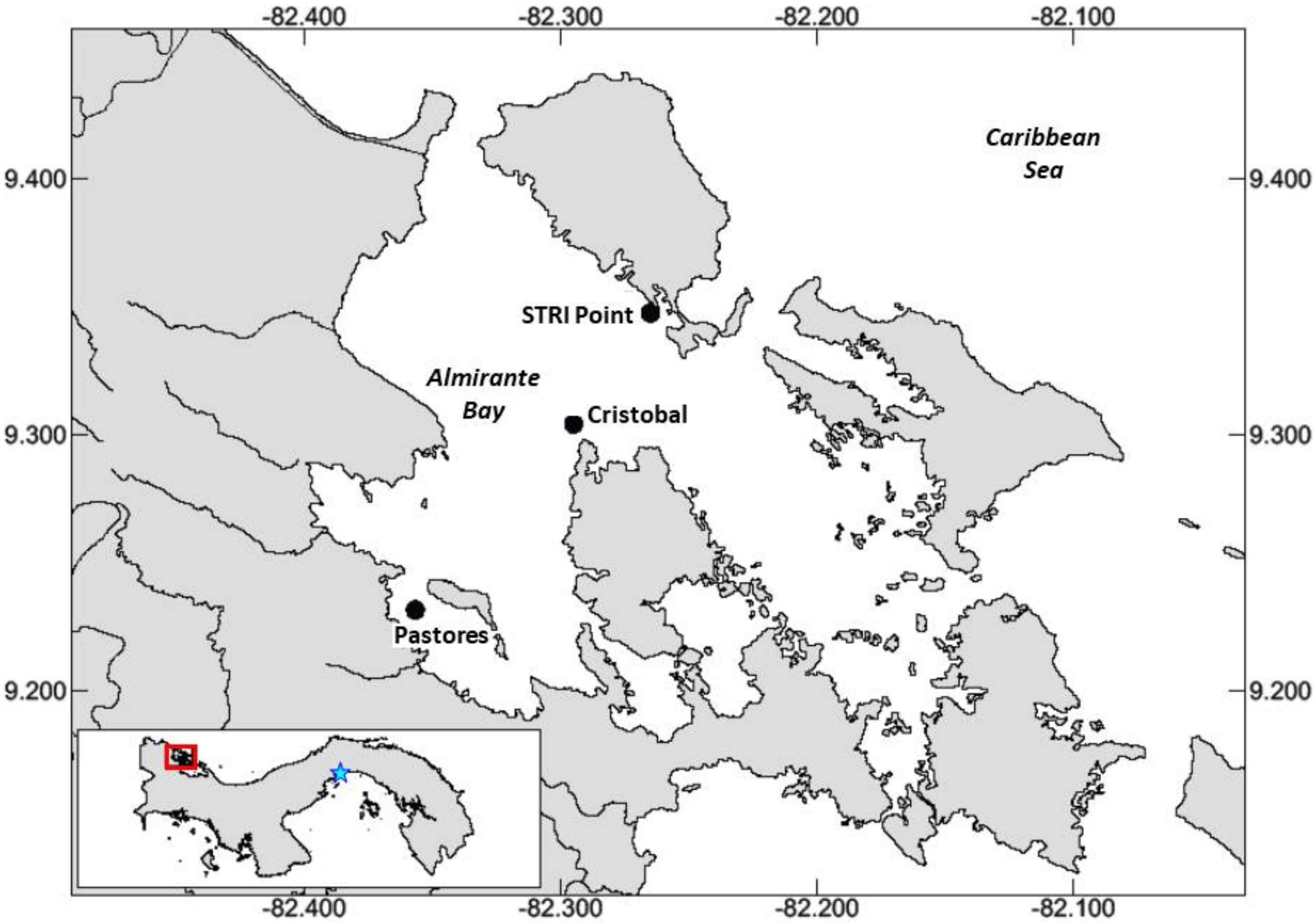
2.1. Study Site
2.2. Sampling
2.3. Analysis
3. Results
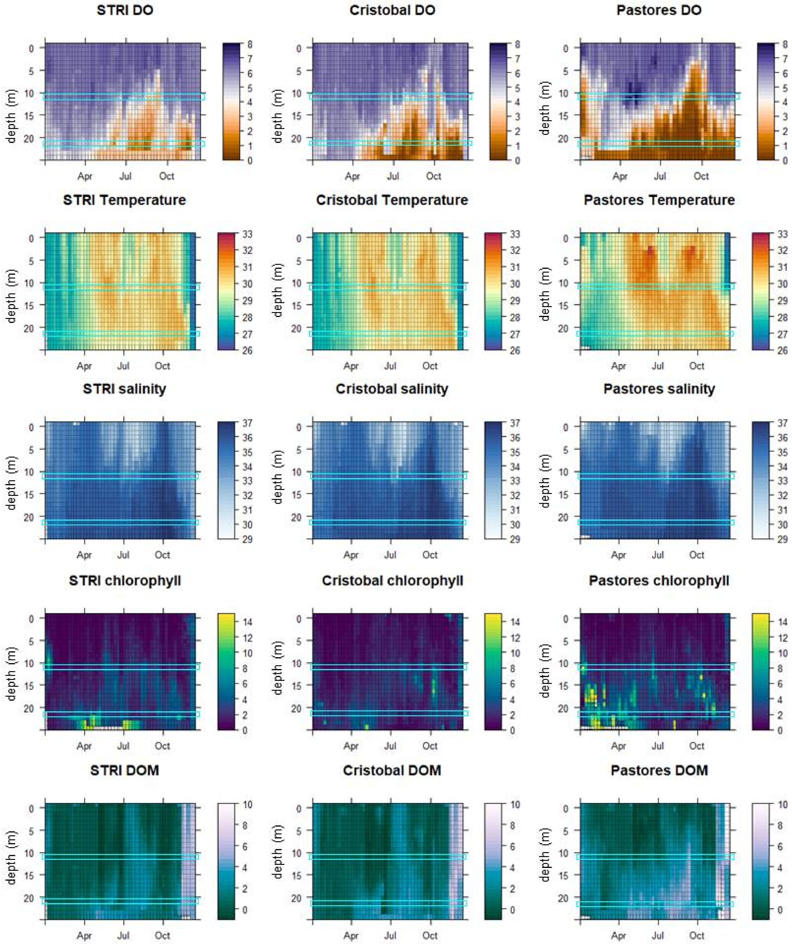
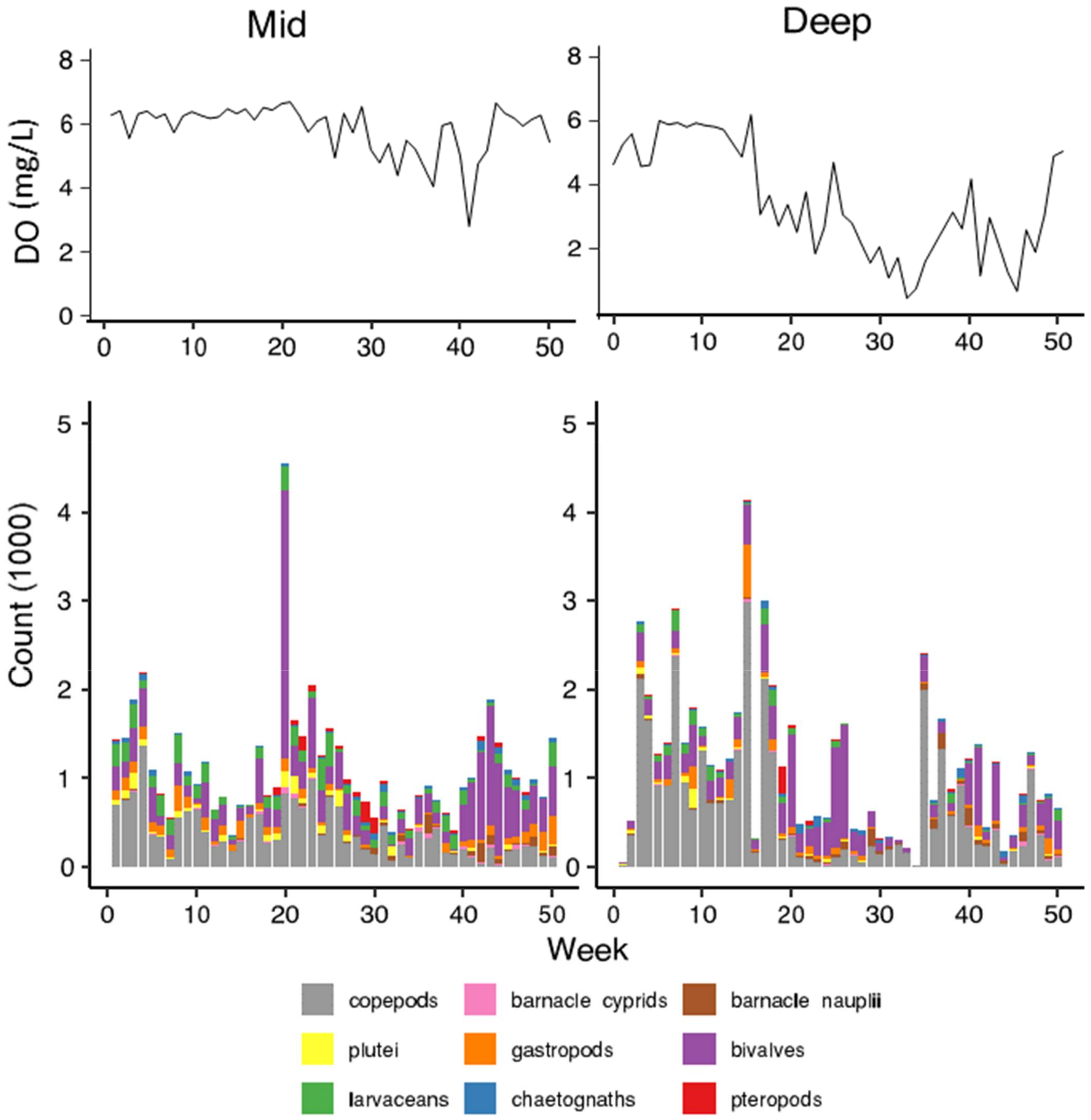
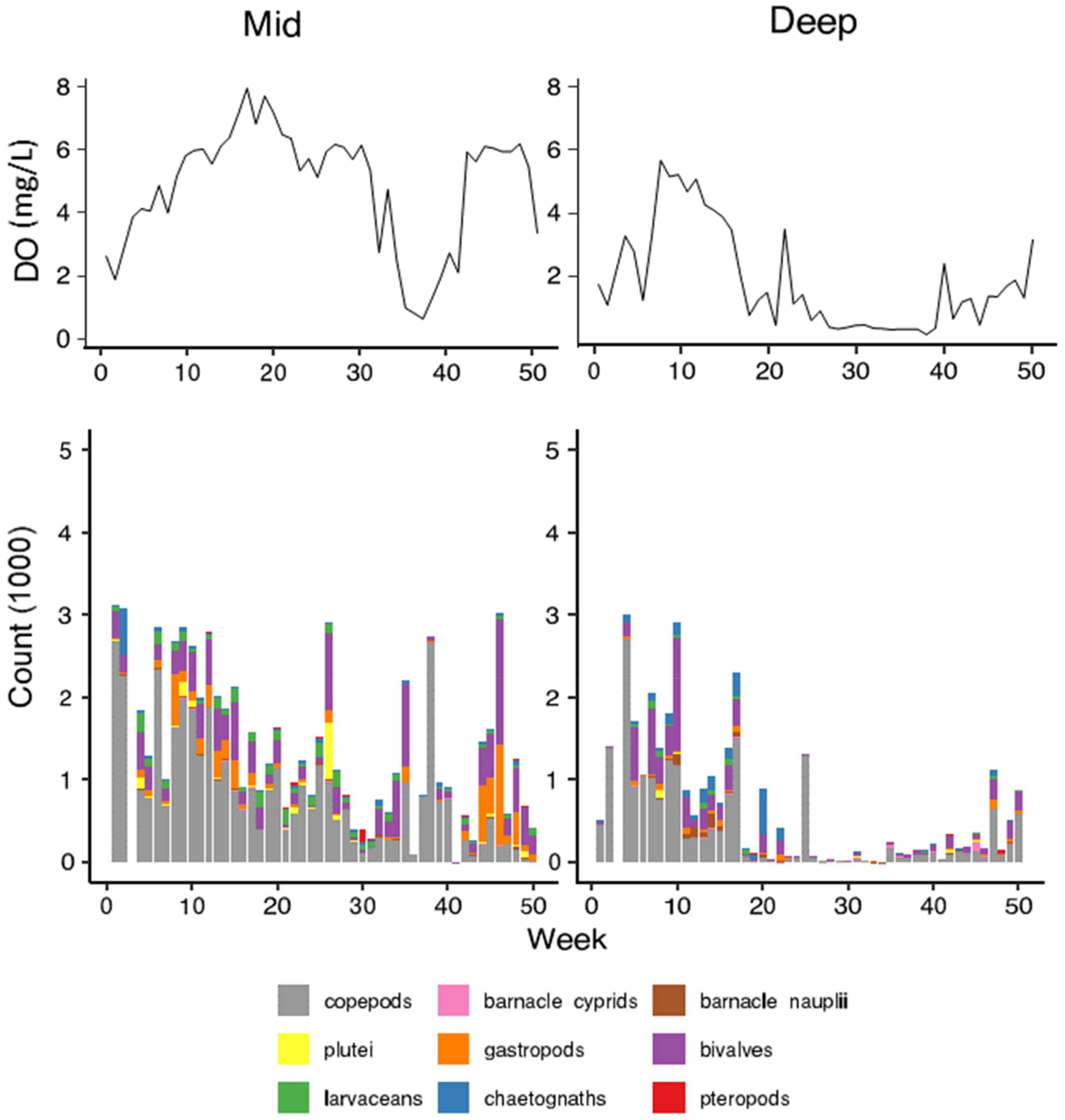
3.1. Environmental Conditions
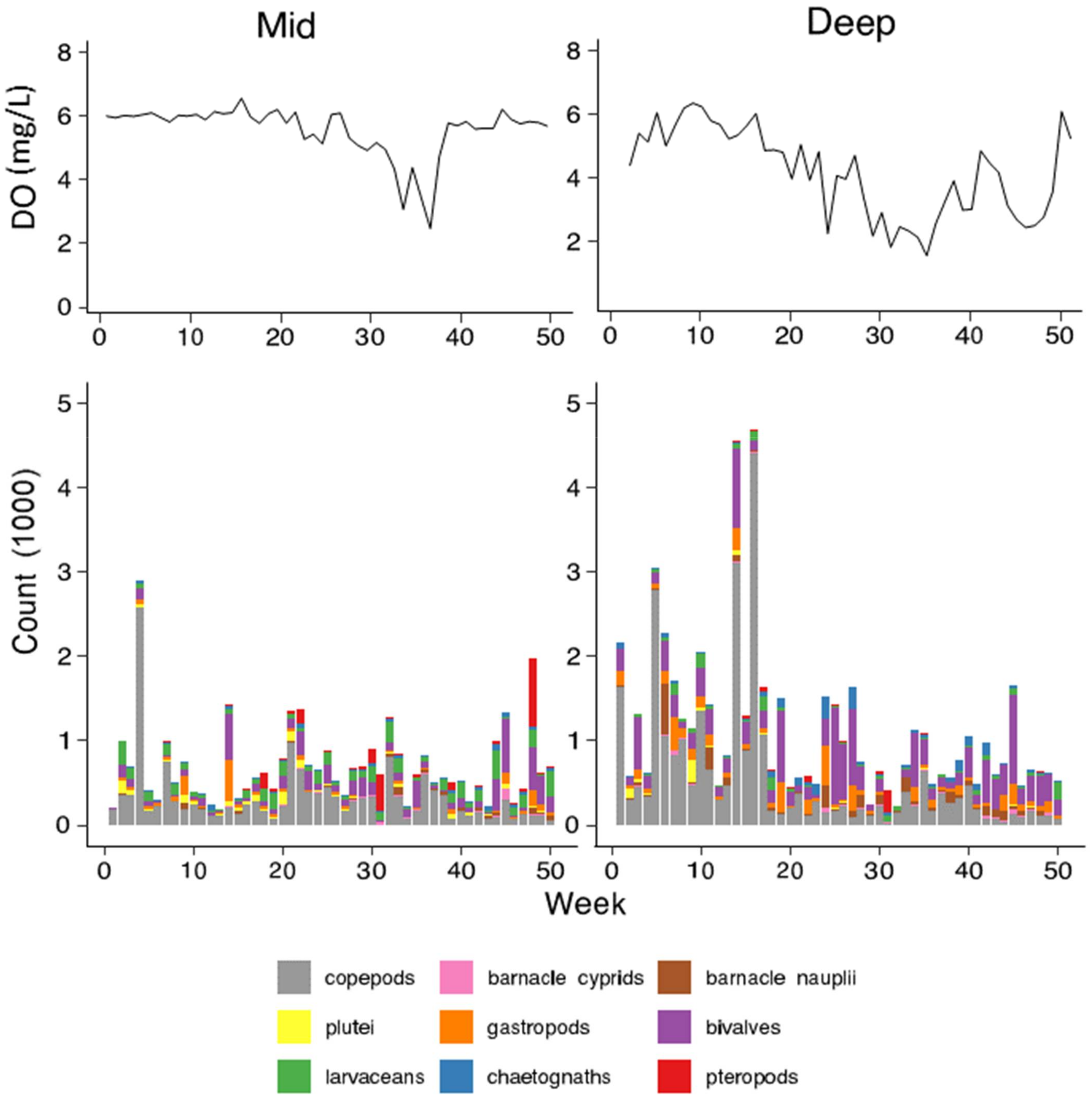
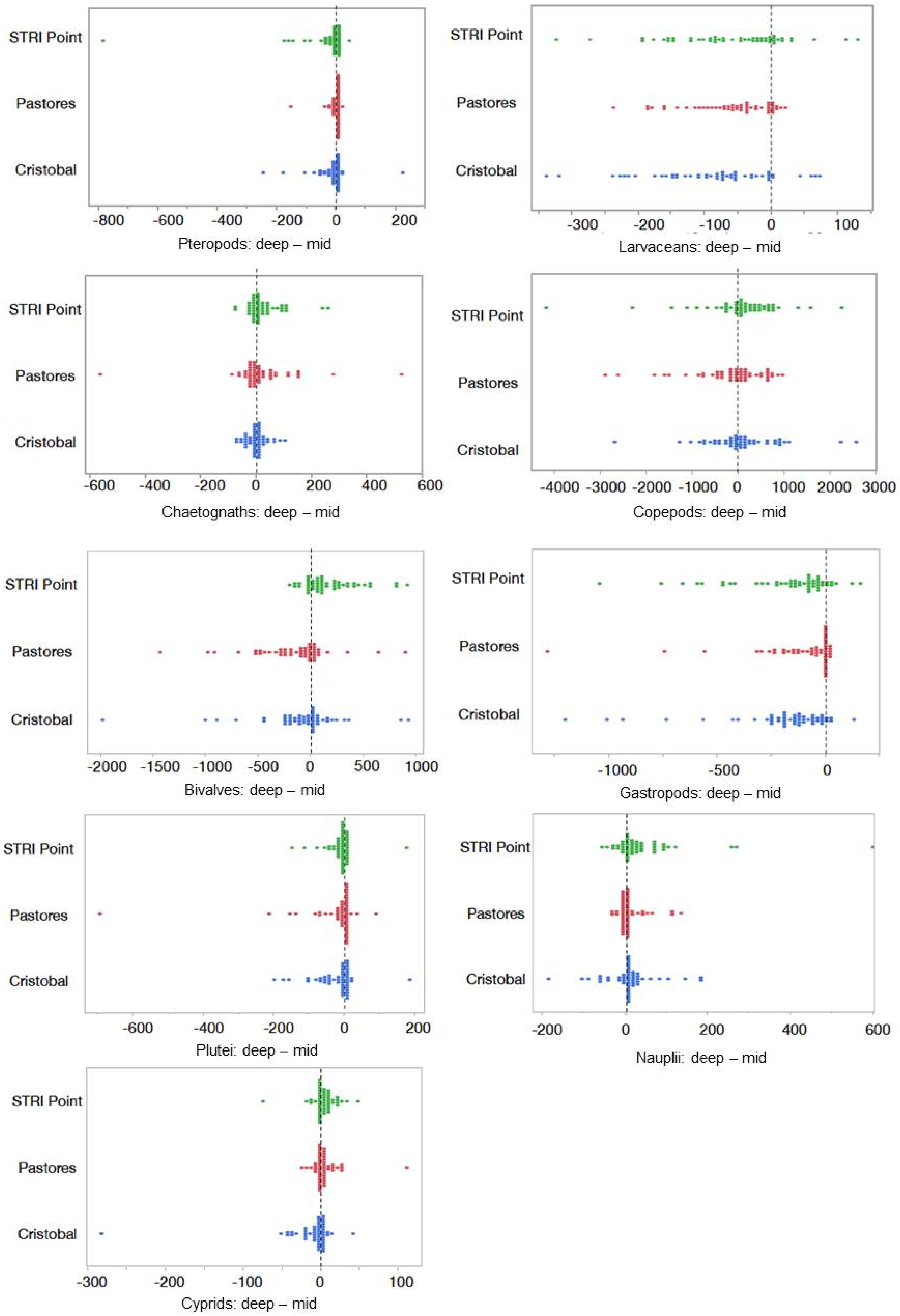
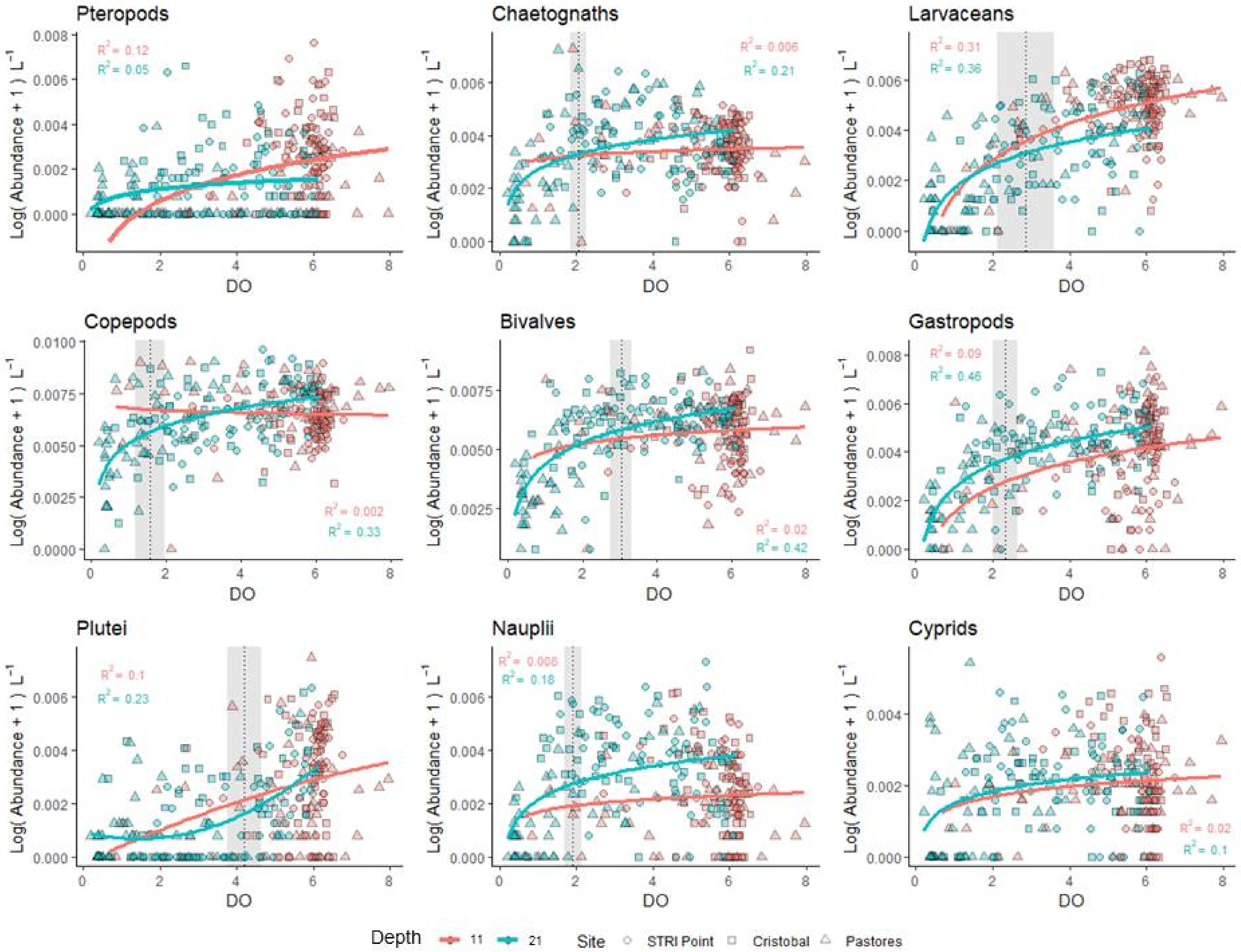
3.2. Patterns of Abundance across Sites and Depths
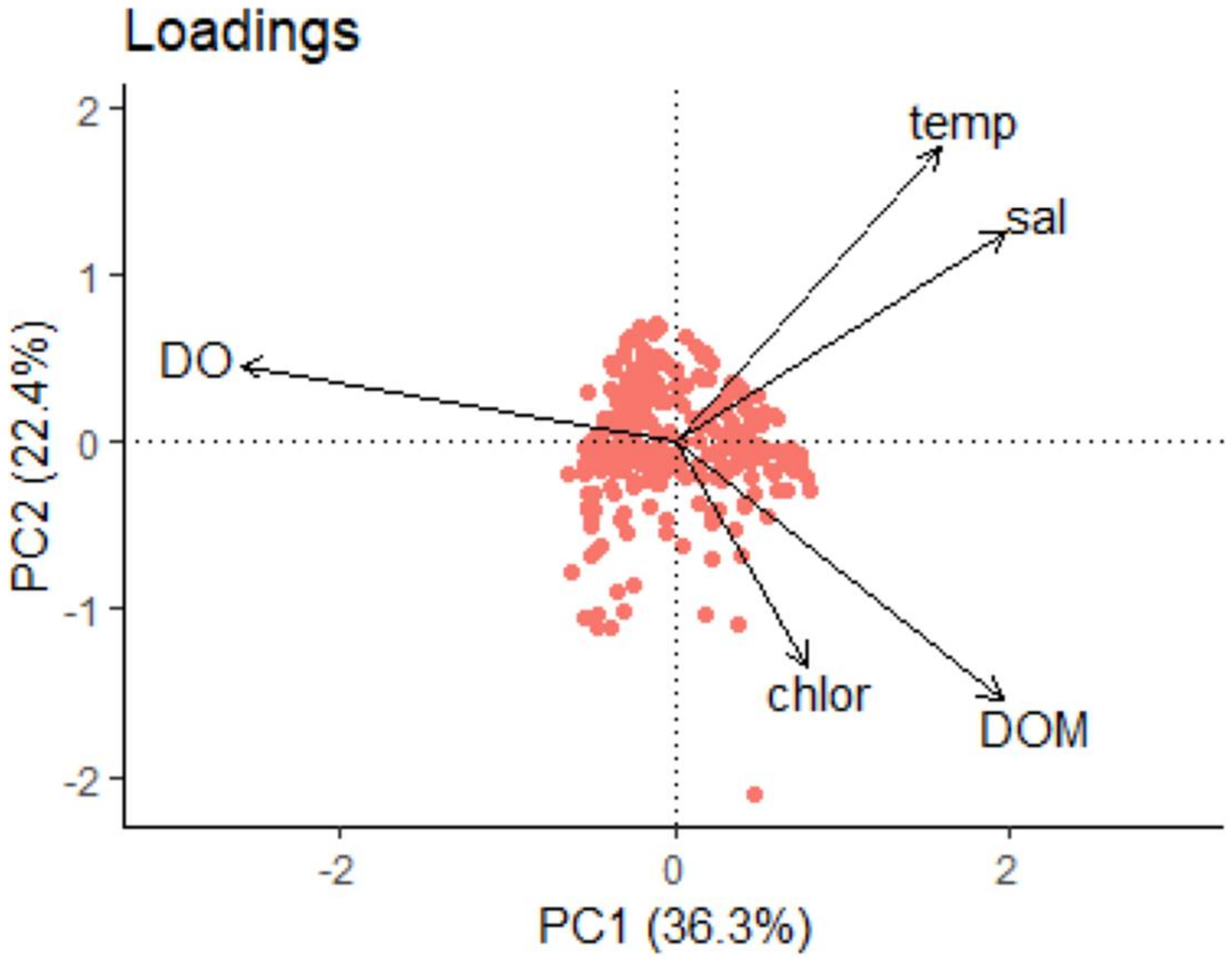
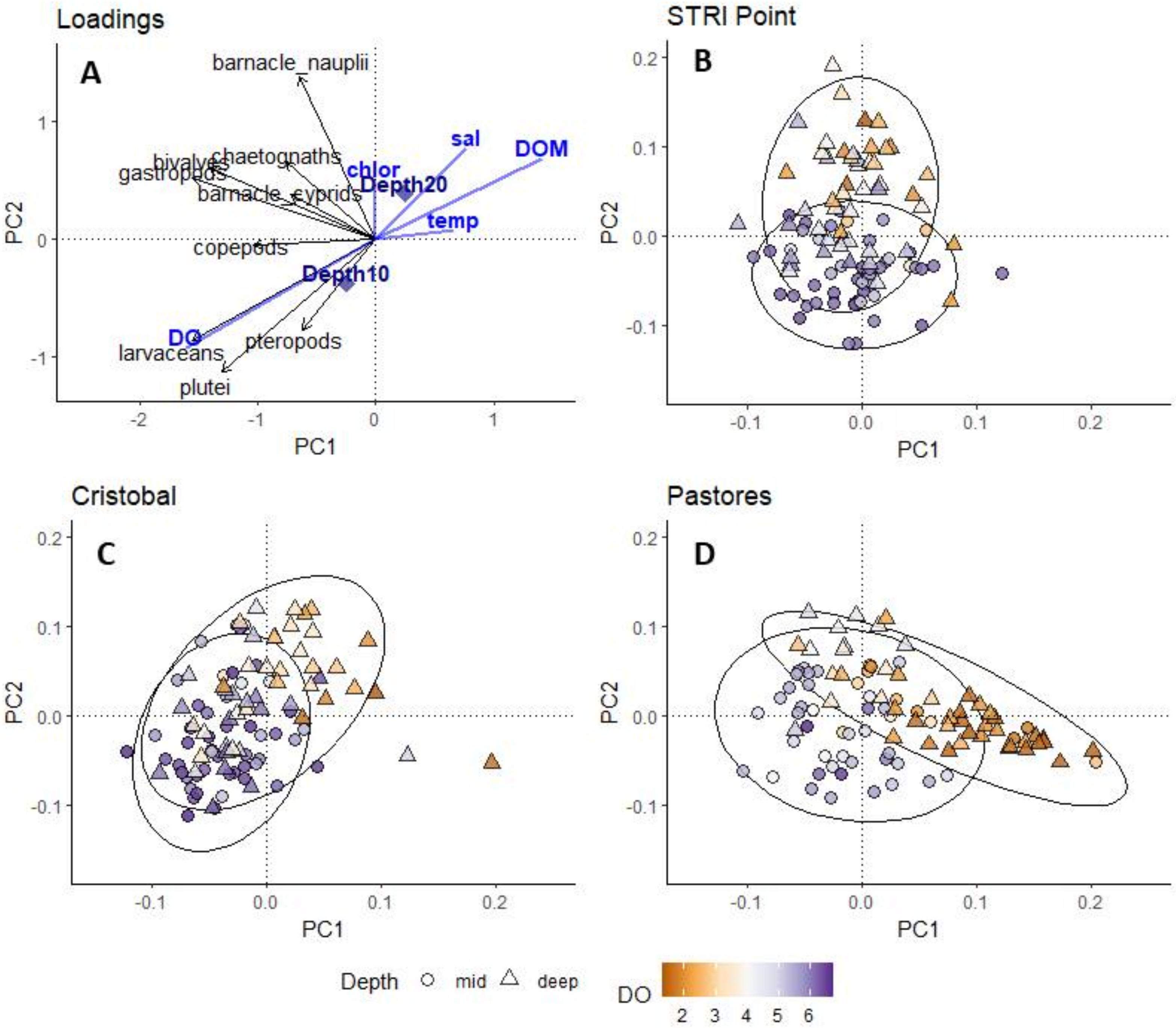
3.3. Total Community Composition and Environmental Factors
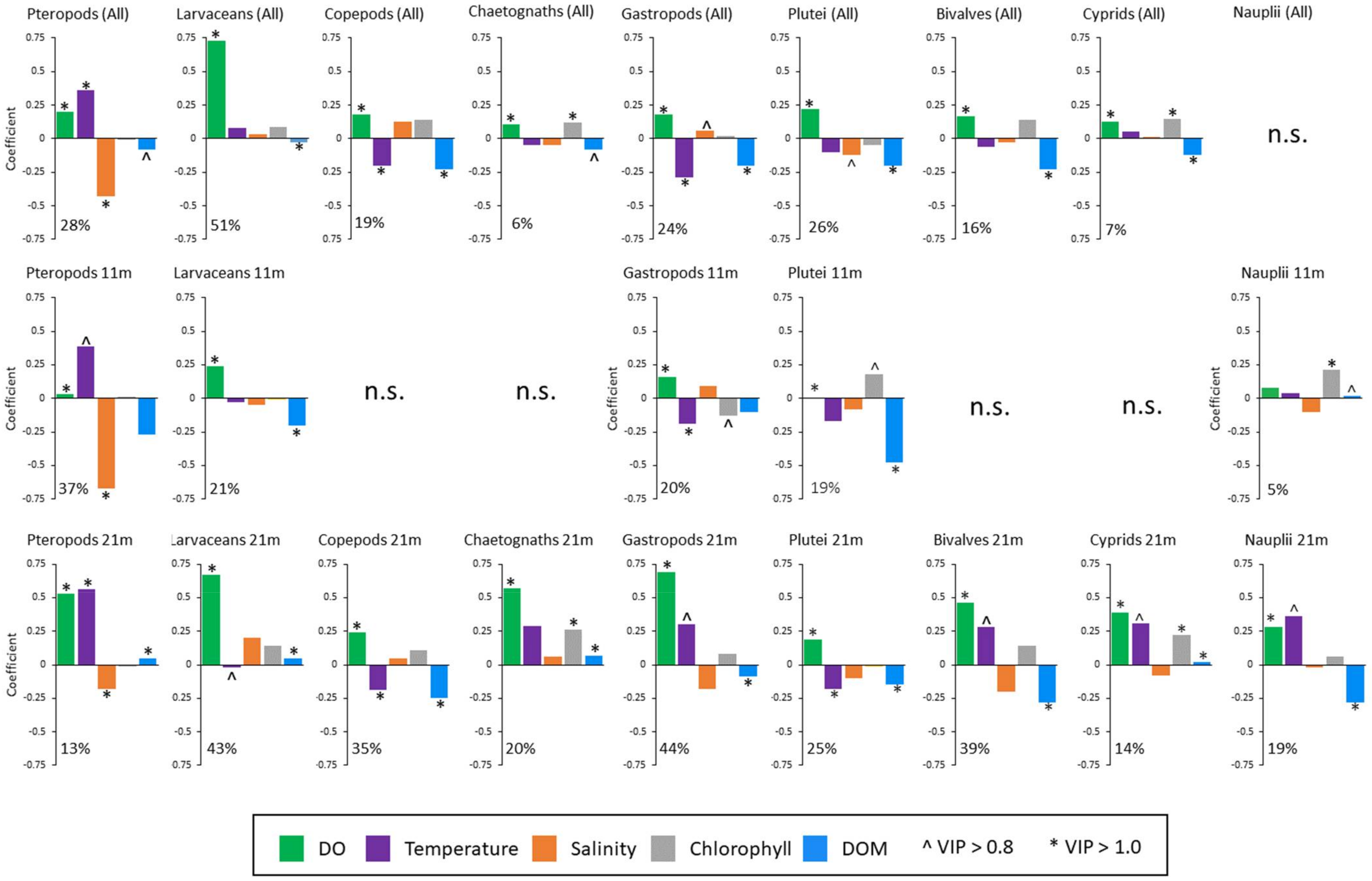
3.4. Environmental Factors Shaping the Abundance of Each Group
4. Discussion
4.1. Impacts of Hypoxia on Plankton and the Almirante Bay Ecosystem
4.2. DOM and Zooplankton in Hypoxic Environments
4.3. Taxon Specific Responses
5. Conclusions
Supplementary Materials
Author Contributions
Funding
Institutional Review Board Statement
Informed Consent Statement
Data Availability Statement
Acknowledgments
Conflicts of Interest
References
- Breitburg, D.; Levin, L.A.; Oschlies, A.; Grégoire, M.; Chavez, F.P.; Conley, D.J.; Garçon, V.; Gilbert, D.; Gutiérrez, D.; Isensee, K.; et al. Declining Oxygen in the Global Ocean and Coastal Waters. Science 2018, 359, eaam7240. [Google Scholar] [CrossRef] [PubMed] [Green Version]
- Stramma, L.; Johnson, G.C.; Sprintall, J.; Mohrholz, V. Expanding Oxygen-Minimum Zones in the Tropical Oceans. Science 2008, 320, 655–658. [Google Scholar] [CrossRef] [PubMed] [Green Version]
- Oschlies, A.; Brandt, P.; Stramma, L.; Schmidtko, S. Drivers and Mechanisms of Ocean Deoxygenation. Nat. Geosci. 2018, 11, 467–473. [Google Scholar] [CrossRef]
- Paerl, H.; Pinckney, J.; Fear, J.; Peierls, B. Ecosystem Responses to Internal and Watershed Organic Matter Loading:Consequences for Hypoxia in the Eutrophying Neuse River Estuary, North Carolina, USA. Mar. Ecol. Prog. Ser. 1998, 166, 17–25. [Google Scholar] [CrossRef] [Green Version]
- Gruber, N. Warming up, Turning Sour, Losing Breath: Ocean Biogeochemistry under Global Change. Philos. Trans. R. Soc. Math. Phys. Eng. Sci. 2011, 369, 1980–1996. [Google Scholar] [CrossRef] [Green Version]
- Doney, S.C.; Ruckelshaus, M.; Emmett Duffy, J.; Barry, J.P.; Chan, F.; English, C.A.; Galindo, H.M.; Grebmeier, J.M.; Hollowed, A.B.; Knowlton, N.; et al. Climate Change Impacts on Marine Ecosystems. Annu. Rev. Mar. Sci. 2012, 4, 11–37. [Google Scholar] [CrossRef] [Green Version]
- Lucey, N.M.; Haskett, E.; Collin, R. Multi-Stressor Extremes Found on a Tropical Coral Reef Impair Performance. Front. Mar. Sci. 2020, 7, 588764. [Google Scholar] [CrossRef]
- Lucey, N.; Deutsch, C.A.; Carignan, M.-H.; Vermandele, F.; Collins, M.; Johnson, M.D.; Collin, R.; Calosi, P. Climate Warming Erodes Tropical Reef Habitat by Increasing Frequency and Intensity of Low Oxygen Extremes. Science, submitted.
- Tewksbury, J.J.; Huey, R.B.; Deutsch, C.A. Putting the Heat on Tropical Animals. Science 2008, 320, 1296–1297. [Google Scholar] [CrossRef]
- Vinagre, C.; Leal, I.; Mendonça, V.; Madeira, D.; Narciso, L.; Diniz, M.S.; Flores, A.A.V. Vulnerability to Climate Warming and Acclimation Capacity of Tropical and Temperate Coastal Organisms. Ecol. Indic. 2016, 62, 317–327. [Google Scholar] [CrossRef]
- Collin, R.; Chan, K.Y.K. The Sea Urchin Lytechinus Variegatus Lives Close to the Upper Thermal Limit for Early Development in a Tropical Lagoon. Ecol. Evol. 2016, 6, 5623–5634. [Google Scholar] [CrossRef] [Green Version]
- Pinsky, M.L.; Eikeset, A.M.; McCauley, D.J.; Payne, J.L.; Sunday, J.M. Greater Vulnerability to Warming of Marine versus Terrestrial Ectotherms. Nature 2019, 569, 108–111. [Google Scholar] [CrossRef] [PubMed]
- Calbet, A.; Landry, M.R. Phytoplankton Growth, Microzooplankton Grazing, and Carbon Cycling in Marine Systems. Limnol. Oceanogr. 2004, 49, 51–57. [Google Scholar] [CrossRef] [Green Version]
- Siegel, D.A.; Buesseler, K.O.; Doney, S.C.; Sailley, S.F.; Behrenfeld, M.J.; Boyd, P.W. Global Assessment of Ocean Carbon Export by Combining Satellite Observations and Food-Web Models. Glob. Biogeochem. Cycles 2014, 28, 181–196. [Google Scholar] [CrossRef]
- Honjo, S.; Manganini, S.J. Annual Biogenic Particle Fluxes to the Interior of the North Atlantic Ocean Studied at 34° N 21° W and 48° N 21° W. Deep Sea Res. Part II Top. Stud. Oceanogr. 1993, 40, 587–607. [Google Scholar] [CrossRef]
- Christiansen, S.; Hoving, H.; Schütte, F.; Hauss, H.; Karstensen, J.; Körtzinger, A.; Schröder, S.; Stemmann, L.; Christiansen, B.; Picheral, M.; et al. Particulate Matter Flux Interception in Oceanic Mesoscale Eddies by the Polychaete Poeobius sp. Limnol. Oceanogr. 2018, 63, 2093–2109. [Google Scholar] [CrossRef] [Green Version]
- Cowen, R.K.; Sponaugle, S. Larval Dispersal and Marine Population Connectivity. Annu. Rev. Mar. Sci. 2009, 1, 443–466. [Google Scholar] [CrossRef] [Green Version]
- Lasker, R. The Role of a Stable Ocean in Larval Fish Survival and Subsequent Recruitment. Mar. Fish Larvae Morphol. Ecol. Relat. Fish. 1981, 1, 80–89. [Google Scholar]
- Breitburg, D.L. Episodic Hypoxia in Chesapeake Bay: Interacting Effects of Recruitment, Behavior, and Physical Disturbance. Ecol. Monogr. 1992, 62, 525–546. [Google Scholar] [CrossRef]
- Milicich, M. Dynamic Coupling of Reef Fish Replenishment and Oceanographic Processes. Mar. Ecol. Prog. Ser. 1994, 110, 135–144. [Google Scholar] [CrossRef]
- Nicholson, G.; Jenkins, G.P.; Sherwood, J.; Longmore, A. Physical Environmental Conditions, Spawning and Early-Life Stages of an Estuarine Fish: Climate Change Implications for Recruitment in Intermittently Open Estuaries. Mar. Freshw. Res. 2008, 59, 735. [Google Scholar] [CrossRef]
- Slater, W.L.; Pierson, J.J.; Decker, M.B.; Houde, E.D.; Lozano, C.; Seuberling, J. Fewer Copepods, Fewer Anchovies, and More Jellyfish: How Does Hypoxia Impact the Chesapeake Bay Zooplankton Community? Diversity 2020, 12, 35. [Google Scholar] [CrossRef] [Green Version]
- Keister, J.E.; Winans, A.K.; Herrmann, B. Zooplankton Community Response to Seasonal Hypoxia: A Test of Three Hypotheses. Diversity 2020, 12, 21. [Google Scholar] [CrossRef] [Green Version]
- Roman, M.R.; Pierson, J.J.; Kimmel, D.G.; Boicourt, W.C.; Zhang, X. Impacts of Hypoxia on Zooplankton Spatial Distributions in the Northern Gulf of Mexico. Estuaries Coasts 2012, 35, 1261–1269. [Google Scholar] [CrossRef]
- Roman, M.R.; Gauzens, A.L.; Rhinehart, W.K.; White, J.R. Effects of Low Oxygen Waters on Chesapeake Bay Zooplankton. Limnol. Oceanogr. 1993, 38, 1603–1614. [Google Scholar] [CrossRef]
- Sato, M.; Horne, J.; Parker-Stetter, S.; Essington, T.; Keister, J.; Moriarty, P.; Li, L.; Newton, J. Impacts of Moderate Hypoxia on Fish and Zooplankton Prey Distributions in a Coastal Fjord. Mar. Ecol. Prog. Ser. 2016, 560, 57–72. [Google Scholar] [CrossRef] [Green Version]
- Qureshi, N.A.; Rabalais, N.N. Distribution of Zooplankton on a Seasonally Hypoxic Continental Shelf. In Coastal and Estuarine Studies; Rabalais, N.N., Turner, R.E., Eds.; American Geophysical Union: Washington, DC, USA, 2001; Volume 58, pp. 61–76. ISBN 978-0-87590-272-2. [Google Scholar]
- Webster, C.N.; Hansson, S.; Didrikas, T.; Gorokhova, E.; Peltonen, H.; Brierley, A.S.; Lehtiniemi, M. Stuck between a Rock and a Hard Place: Zooplankton Vertical Distribution and Hypoxia in the Gulf of Finland, Baltic Sea. Mar. Biol. 2015, 162, 1429–1440. [Google Scholar] [CrossRef]
- Kehayias, G.; Aposporis, M. Zooplankton Variation in Relation to Hydrology in an Enclosed Hypoxic Bay (Amvrakikos Gulf, Greece). Mediterr. Mar. Sci. 2014, 15, 554. [Google Scholar] [CrossRef] [Green Version]
- Lučić, D.; Hure, M.; Bobanović-Ćolić, S.; Njire, J.; Vidjak, O.; Onofri, I.; Gangai Zovko, B.; Batistić, M. The Effect of Temperature Change and Oxygen Reduction on Zooplankton Composition and Vertical Distribution in a Semi-Enclosed Marine System. Mar. Biol. Res. 2019, 15, 325–342. [Google Scholar] [CrossRef]
- Weinstock, J.B.; Collin, R. Hypoxia and Warming Are Associated with Reductions in Larval Bivalve Abundance in a Tropical Lagoon. Mar. Ecol. Prog. Ser. 2021, 662, 85–95. [Google Scholar] [CrossRef]
- Wiebe, P.H. Small-Scale Spatial Distribution in Oceanic Zooplankton. Limnol. Oceanogr. 1970, 15, 205–217. [Google Scholar] [CrossRef]
- Décima, M.; Ohman, M.D.; Robertis, A.D. Body Size Dependence of Euphausiid Spatial Patchiness. Limnol. Oceanogr. 2010, 55, 777–788. [Google Scholar] [CrossRef]
- Greb, L.; Saric, B.; Seyfried, H.; Broszonn, T.; Brauch, S.; Gugau, G.; Wiltschko, C.; Leinfelder, R. Profil: Ökologie und Sedimentologie Eines Rezenten Rampensystem an der Karibikküste von Panamá; Universität Stuttgart: Stuttgart, Germany, 1996; Volume 10. [Google Scholar]
- Guzmán, H.M.; Barnes, P.A.G.; Lovelock, C.E.; Feller, I.C. A Site Description of the CARICOMP Mangrove, Seagrass and Coral Reef Sites in Bocas Del Toro, Panama. Caribb. J. Sci. 2005, 41, 430–440. [Google Scholar]
- Adelson, A.E.; Altieri, A.H.; Collin, R.; Davis, K.A.; Gaul, A.; Giddings, S.N.; Reed, V.; Pawlak, G. Hydrography of Hypoxic Events and Temperature Inversions in Bahía Almirante, a Shallow Tropical Embayment in Bocas Del Toro, Panama. Limnol. Oceanogr. submitted.
- Kaufmann, K.W.; Thompson, R.C. Water Temperature Variation and the Meteorological and Hydrographic Environment of Bocas Del Toro, Panama. Caribb. J. Sci. 2005, 41, 392–413. [Google Scholar]
- Neal, B.P.; Condit, C.; Liu, G.; dos Santos, S.; Kahru, M.; Mitchell, B.G.; Kline, D.I. When Depth Is No Refuge: Cumulative Thermal Stress Increases with Depth in Bocas Del Toro, Panama. Coral Reefs 2014, 33, 193–205. [Google Scholar] [CrossRef] [Green Version]
- Altieri, A.H.; Harrison, S.B.; Seemann, J.; Collin, R.; Diaz, R.J.; Knowlton, N. Tropical Dead Zones and Mass Mortalities on Coral Reefs. Proc. Natl. Acad. Sci. USA 2017, 114, 3660–3665. [Google Scholar] [CrossRef] [Green Version]
- Johnson, M.D.; Scott, J.J.; Leray, M.; Lucey, N.; Bravo, L.M.R.; Wied, W.L.; Altieri, A.H. Rapid Ecosystem-Scale Consequences of Acute Deoxygenation on a Caribbean Coral Reef. Nat. Commun. 2021, 12, 4522. [Google Scholar] [CrossRef]
- Lucey, N.M.; Collins, M.; Collin, R. Oxygen-mediated Plasticity Confers Hypoxia Tolerance in a Corallivorous Polychaete. Ecol. Evol. 2020, 10, 1145–1157. [Google Scholar] [CrossRef] [Green Version]
- Sarkar, D.; Andrews, F. LatticeExtra: Extra Graphical Utilities Based on Lattice, R package version 0.6-26. 2019.
- Oksanen, J.; Blanchet, F.G.; Friendly, M.; Kindt, R.; Legendre, P.; McGlinn, D.; Minchin, P.R.; O’Hara, R.B.; Simpson, G.L.; Solymos, P.; et al. Vegan: Community Ecology Package, R package version 2.5-7. 2020.
- Wang, Y.; Naumann, U.; Wright, S.T.; Warton, D.I. Mvabund—An R Package for Model-Based Analysis of Multivariate Abundance Data: The Mvabund R Package. Methods Ecol. Evol. 2012, 3, 471–474. [Google Scholar] [CrossRef]
- Wang, Y.; Naumann, U.; Eddelbuettel, D.; Wilshire, J.; Warton, D. Mvabund: Statistical Methods for Analysing Multivariate Abundance Data, R package version 4.1.12. 2021.
- Venables, W.N.; Ripley, B.D. Modern Applied Statistics with S; Springer: New York, NY, USA, 2002. [Google Scholar]
- Carrascal, L.M.; Galván, I.; Gordo, O. Partial Least Squares Regression as an Alternative to Current Regression Methods Used in Ecology. Oikos 2009, 118, 681–690. [Google Scholar] [CrossRef]
- Mehmood, T.; Liland, K.H.; Snipen, L.; Sæbø, S. A Review of Variable Selection Methods in Partial Least Squares Regression. Chemom. Intell. Lab. Syst. 2012, 118, 62–69. [Google Scholar] [CrossRef]
- Muggeo, V.M.R. Segmented: An R Package to Fit Regression Models with Broken-Line Relationships, R package version 1.4-0. 2008.
- R Core Team. R: A Language and Environment for Statistical Computing; R Foundation for Statistical Computing: Vienna, Austria, 2021. [Google Scholar]
- Baumann, H.; Smith, E.M. Quantifying Metabolically Driven PH and Oxygen Fluctuations in US Nearshore Habitats at Diel to Interannual Time Scales. Estuaries Coasts 2018, 41, 1102–1117. [Google Scholar] [CrossRef]
- Diaz, R.J. Overview of Hypoxia around the World. J. Environ. Qual. 2001, 30, 275–281. [Google Scholar] [CrossRef] [PubMed]
- Bopp, L.; Resplandy, L.; Orr, J.C.; Doney, S.C.; Dunne, J.P.; Gehlen, M.; Halloran, P.; Heinze, C.; Ilyina, T.; Séférian, R.; et al. Multiple Stressors of Ocean Ecosystems in the 21st Century: Projections with CMIP5 Models. Biogeosciences 2013, 10, 6225–6245. [Google Scholar] [CrossRef] [Green Version]
- Guadayol, Ò.; Silbiger, N.J.; Donahue, M.J.; Thomas, F.I.M. Patterns in Temporal Variability of Temperature, Oxygen and PH along an Environmental Gradient in a Coral Reef. PLoS ONE 2014, 9, e85213. [Google Scholar] [CrossRef] [PubMed] [Green Version]
- Gobler, C.J.; Baumann, H. Hypoxia and Acidification in Ocean Ecosystems: Coupled Dynamics and Effects on Marine Life. Biol. Lett. 2016, 12, 20150976. [Google Scholar] [CrossRef] [PubMed] [Green Version]
- Levin, L.A.; Ekau, W.; Gooday, A.J.; Jorissen, F.; Middelburg, J.J.; Naqvi, S.W.A.; Neira, C.; Rabalais, N.N.; Zhang, J. Effects of Natural and Human-Induced Hypoxia on Coastal Benthos. Biogeosciences 2009, 6, 2063–2098. [Google Scholar] [CrossRef] [Green Version]
- Diaz, R.J.; Rosenberg, R. Marine Benthic Hypoxia: A Review of Its Ecological Effects and the Behavioural Responses of Benthic Macrofauna. Oceanogr. Mar. Biol. Annu. Rev. 1995, 33, 245–303. [Google Scholar]
- Gray, J.; Wu, R.; Or, Y. Effects of Hypoxia and Organic Enrichment on the Coastal Marine Environment. Mar. Ecol. Prog. Ser. 2002, 238, 249–279. [Google Scholar] [CrossRef]
- Vaquer-Sunyer, R.; Duarte, C.M. Thresholds of Hypoxia for Marine Biodiversity. Proc. Natl. Acad. Sci. USA 2008, 105, 15452–15457. [Google Scholar] [CrossRef] [Green Version]
- Roman, M.R.; Brandt, S.B.; Houde, E.D.; Pierson, J.J. Interactive Effects of Hypoxia and Temperature on Coastal Pelagic Zooplankton and Fish. Front. Mar. Sci. 2019, 6, 139. [Google Scholar] [CrossRef] [Green Version]
- Somero, G.N.; Beers, J.M.; Chan, F.; Hill, T.M.; Klinger, T.; Litvin, S.Y. What Changes in the Carbonate System, Oxygen, and Temperature Portend for the Northeastern Pacific Ocean: A Physiological Perspective. BioScience 2016, 66, 14–26. [Google Scholar] [CrossRef] [Green Version]
- Howard, E.M.; Penn, J.L.; Frenzel, H.; Seibel, B.A.; Bianchi, D.; Renault, L.; Kessouri, F.; Sutula, M.A.; McWilliams, J.C.; Deutsch, C. Climate-Driven Aerobic Habitat Loss in the California Current System. Sci. Adv. 2020, 6, eaay3188. [Google Scholar] [CrossRef] [PubMed]
- Jessen, C.; Bednarz, V.N.; Rix, L.; Teichberg, M.; Wild, C. Marine Eutrophication. In Environmental Indicators; Armon, R.H., Hänninen, O., Eds.; Springer Netherlands: Dordrecht, The Netherlands, 2015; pp. 177–203. ISBN 978-94-017-9498-5. [Google Scholar]
- Howarth, R.; Chan, F.; Conley, D.J.; Garnier, J.; Doney, S.C.; Marino, R.; Billen, G. Coupled Biogeochemical Cycles: Eutrophication and Hypoxia in Temperate Estuaries and Coastal Marine Ecosystems. Front. Ecol. Environ. 2011, 9, 18–26. [Google Scholar] [CrossRef] [Green Version]
- Middelburg, J.J.; Levin, L.A. Coastal Hypoxia and Sediment Biogeochemistry. Biogeosciences 2009, 6, 1273–1293. [Google Scholar] [CrossRef] [Green Version]
- Dupont, S.; Dorey, N.; Thorndyke, M. What Meta-Analysis Can Tell Us about Vulnerability of Marine Biodiversity to Ocean Acidification? Estuar. Coast. Shelf Sci. 2010, 89, 182–185. [Google Scholar] [CrossRef]
- Mohammed, A. Why Are Early Life Stages of Aquatic Organisms More Sensitive to Toxicants than Adults? In New Insights into Toxicity and Drug Testing; Gowder, S., Ed.; InTech: Rijeka, Croatia, 2013; ISBN 978-953-51-0946-4. [Google Scholar]
- Pandori, L.L.M.; Sorte, C.J.B. The Weakest Link: Sensitivity to Climate Extremes across Life Stages of Marine Invertebrates. Oikos 2019, 128, 621–629. [Google Scholar] [CrossRef] [Green Version]
- Mustaffa, N.I.H.; Kallajoki, L.; Biederbick, J.; Binder, F.I.; Schlenker, A.; Striebel, M. Coastal Ocean Darkening Effects via Terrigenous DOM Addition on Plankton: An Indoor Mesocosm Experiment. Front. Mar. Sci. 2020, 7, 547829. [Google Scholar] [CrossRef]
- Manahan, D.T. Adaptations by Invertebrate Larvae for Nutrient Acquisition from Seawater. Am. Zool. 1990, 30, 147–160. [Google Scholar] [CrossRef] [Green Version]
- Jaeckle, W.B.; Manahan, D.T. Experimental Manipulations of the Organic Composition of Seawater: Implications for Studies of Energy Budgets in Marine Invertebrate Larvae. J. Exp. Mar. Biol. Ecol. 1992, 156, 273–284. [Google Scholar] [CrossRef]
- Kiørboe, T. How Zooplankton Feed: Mechanisms, Traits and Trade-Offs. Biol. Rev. 2011, 86, 311–339. [Google Scholar] [CrossRef]
- Vanderploeg, H.A. Zooplankton Particle Selection and Feeding Mechanisms. In The Biology of Particles in Aquatic Systems; CRC Press: Boca Raton, FL, USA, 2020; pp. 205–234. [Google Scholar]
- Sunday, J.M.; Pecl, G.T.; Frusher, S.; Hobday, A.J.; Hill, N.; Holbrook, N.J.; Edgar, G.J.; Stuart-Smith, R.; Barrett, N.; Wernberg, T.; et al. Species Traits and Climate Velocity Explain Geographic Range Shifts in an Ocean-Warming Hotspot. Ecol. Lett. 2015, 18, 944–953. [Google Scholar] [CrossRef] [PubMed]
- Stuart-Smith, R.D.; Edgar, G.J.; Bates, A.E. Thermal Limits to the Geographic Distributions of Shallow-Water Marine Species. Nat. Ecol. Evol. 2017, 1, 1846–1852. [Google Scholar] [CrossRef] [PubMed]
- Deutsch, C.; Ferrel, A.; Seibel, B.; Pörtner, H.-O.; Huey, R.B. Climate Change Tightens a Metabolic Constraint on Marine Habitats. Science 2015, 348, 1132–1135. [Google Scholar] [CrossRef] [PubMed] [Green Version]


| STRI | Cristobal | Pastores | |
|---|---|---|---|
| Pteropods | 0.30 ** | 0.23 * | 0.33 ** |
| Chaetognaths | −0.04 | 0.03 | −0.04 |
| Larvaceans | 0.11 | 0.31 | 0.11 |
| Copepods | 0.10 | 0.04 | 0.15 |
| Bivalves | 0.12 | 0.30 ** | 0.24 * |
| Gastropods | 0.25 * | 0.39 *** | 0.41 *** |
| Plutei | 0.41 *** | 0.45 *** | 0.27 * |
| Nauplii | 0.16 | 0.40 *** | 0.16 |
| Cyprids | 0.20 | 0.24 * | 0.21 * |
| Variable | Resid. Df | Df | Dev | Pr(>Dev) |
|---|---|---|---|---|
| Depth (mid or deep) | 292 | 1 | 124.56 | 0.001 *** |
| DO | 291 | 1 | 203.63 | 0.001 *** |
| Temperature | 290 | 1 | 26.02 | 0.083 |
| Salinity | 289 | 1 | 46.76 | 0.001 ** |
| Chlorophyll | 288 | 1 | 57.70 | 0.001 *** |
| DOM | 287 | 1 | 14.89 | 0.326 |
| DO:Temperature | 286 | 1 | 34.96 | 0.007 ** |
| DO:Chlorophyll | 285 | 1 | 28.13 | 0.030 * |
| DO:DOM | 284 | 1 | 164.69 | 0.002 ** |
| Temperature:Salinity | 283 | 1 | 41.22 | 0.005 ** |
| Holoplankton | Meroplankton | ||||||||
|---|---|---|---|---|---|---|---|---|---|
| Predictors | Pter | Chaet | Larvac | Copep | Bivalves | Gastr | Plutei | Nauplii | Cyprids |
| Depth (deep) | * | ** | * | * | ** | ||||
| DO | n.s. | ** | * | * | *** | *** | *** | *** | n.s. |
| Temperature | *** | ** | * | ** | * | *** | ** | *** | |
| Salinity | *** | * | * | *** | * | ** | * | ** | |
| Chlorophyll | n.s. | *** | * | * | * | ** | n.s. | ||
| DOM | *** | *** | n.s. | n.s. | n.s. | n.s. | *** | ** | |
| DO:Temp | *** | ** | * | *** | *** | *** | |||
| DO:Sal | *** | * | |||||||
| DO:Chlor | * | ** | * | ||||||
| DO:DOM | *** | *** | *** | *** | *** | *** | *** | ||
| Temp:Sal | * | *** | * | *** | ** | ||||
| Temp:Chlor | * | * | * | ||||||
| Temp:DOM | ** | * | ** | *** | *** | ||||
| Sal:Chlor | * | *** | * | ||||||
| Sal:DOM | ** | * | * | *** | |||||
| Chlor:DOM | * | *** | ** | ||||||
| Overall fit | 25.84% | 23.65% | 40.61% | 19.31% | 20.45% | 24.49% | 25.76% | 23.80% | 15.96% |
Publisher’s Note: MDPI stays neutral with regard to jurisdictional claims in published maps and institutional affiliations. |
© 2022 by the authors. Licensee MDPI, Basel, Switzerland. This article is an open access article distributed under the terms and conditions of the Creative Commons Attribution (CC BY) license (https://creativecommons.org/licenses/by/4.0/).
Share and Cite
Weinstock, J.B.; Vargas, L.; Collin, R. Zooplankton Abundance Reflects Oxygen Concentration and Dissolved Organic Matter in a Seasonally Hypoxic Estuary. J. Mar. Sci. Eng. 2022, 10, 427. https://doi.org/10.3390/jmse10030427
Weinstock JB, Vargas L, Collin R. Zooplankton Abundance Reflects Oxygen Concentration and Dissolved Organic Matter in a Seasonally Hypoxic Estuary. Journal of Marine Science and Engineering. 2022; 10(3):427. https://doi.org/10.3390/jmse10030427
Chicago/Turabian StyleWeinstock, Jane B., Lourdes Vargas, and Rachel Collin. 2022. "Zooplankton Abundance Reflects Oxygen Concentration and Dissolved Organic Matter in a Seasonally Hypoxic Estuary" Journal of Marine Science and Engineering 10, no. 3: 427. https://doi.org/10.3390/jmse10030427