Article

Impacts of River Discharge on the Sea Temperature in Changjiang Estuary and Its Adjacent Sea

1
Institute of Port and Offshore Engineering, Ocean College, Zhejiang University, Zhoushan 316021, China
2
Marine Monitoring and Forecasting Center of Zhejiang Province, Hangzhou 310007, China
3
Department of Civil and Environmental Engineering, University of Washington, Seattle, WA 98195, USA
*
Author to whom correspondence should be addressed.
J. Mar. Sci. Eng. 2022, 10(3), 343; https://doi.org/10.3390/jmse10030343
Submission received: 30 December 2021 / Revised: 8 February 2022 / Accepted: 21 February 2022 / Published: 1 March 2022
(This article belongs to the Special Issue Numerical Modelling Applied for Marine Environmental Sustainability)

Abstract

:
Freshwater plume at the Changjiang River (CR) mouth are essential to the coastal water quality and ecosystem because they can cause estuary stratification and hypoxia, potentially deteriorating the water environment. Furthermore, the advection heat transport is modulated by increasing anthropogenic effects. A comprehensive understanding of the influence of river discharge on the three-dimensional sea temperature, fronts and thermal stratification in the CR estuary remains lacking. A well-calibrated numerical model using Regional Ocean Modeling Systems (ROMS) is used to investigate the impacts of CR discharge on the sea temperature in coastal zones. Model results show that the amplitude and spatial distribution of the heating or cooling rate can be influenced by CR freshwater, especially in frontal areas. Specifically, the large runoff flow will reduce the heating or cooling rate in shallow waters (<20 m) near the CR estuary, whereas it has an opposite effect on the Zhoushan islands region (>20 m). Generally, the effect of the freshwater discharge on the upper layer is greater than on the bottom layer, and the runoff has a positive correlation to the intensity of the frontal zones in the CR estuary, though this relationship is weakened in autumn because of the weak intensity of the frontal zone. Note that seawater thermal stratification and its seasonal variation can be regulated by runoff; thermal stratification will be strengthened in abundant runoff conditions and weakened in scarce runoff conditions.

1. Introduction

The Changjiang River (CR) estuary and its adjacent sea is the largest estuary along the coast of the East China Sea (Figure 1). CR, as the third-largest river in the world, is by far one of the most important ways of discharging water and sediment directly into an estuary. The annual amount of freshwater discharge of CR can reach 31,900 m3/s, with a significant seasonal variation [1,2,3]. The hydrodynamics in the CR estuary and its adjacent sea are influenced by various factors, such as river discharge, atmospheric forcing and tidal mixing. Among these factors, the effect of freshwater has dominated the surface distribution of water properties [1,4].
The Changjiang runoff, which is mixed with inshore seawater and known as the Changjiang diluted water (CDW), is mainly distributed along the Jiangsu and Zhejiang coast adjacent to the Changjiang estuary [5]. In winter, the CDW forms a narrow freshwater band along China’s southeast coast; in summer, it extends northeastward toward Jeju Island [6]. Because of its significant influence, it has been extensively studied based on field observations [2,4], satellite data such as MODIS and SeaWiFS [7] and numerical models [5,6,8,9]. In particular, previous research focused not only on the variety of CDW but also on the impact of CDW on the hydrological cycle [10,11,12] and the ecological environment [13,14,15]. The influences of CDW on environmental consequences that changed systematically after the building of the mega estuarine constructions are also considered [16].
Regarding the environmental effects of CDW, a key indicator of CDW influence on hypoxic zones, and the mixing and transport process in estuaries is seawater temperature (SWT) [11,12,17]. Furthermore, the characteristics of SWT such as front, warm, and cold tongue are good indicators of a marine ecosystem and hydrodynamic processes. As demonstrated in the previous study, the transition between a stratified structure formed by the influence of local sea surface heat flux and river diluted water and unstratified regimes are essentially controlled by the level of tidal mixing, resulting in the relative consistency of the SWT position [18]. The horizontal distribution of water properties in the CR estuary and its adjacent sea is dominated by a temperature tongue or plume of relatively fresh water, especially during the summer when the river output is highest [1,4]. Such a seasonal variation highlights the influence of runoffs on water properties [7,19]. A numerical model was used to study the seasonal variation of the CR estuary’s water temperature structure [9], but the mechanisms of water temperature variation, especially the effects of runoff, have not been studied further.
As a general rule, physical, chemical and biological processes in coastal environments are affected by a change in temperature, especially in frontal zones. Owing to temperature fronts representing the boundaries between different water masses, it plays a significant role in material exchange between the water masses and determines the overall health of aquatic ecosystems [10,20]. Furthermore, the advection heat transport in the CR estuary is modulated by increasing anthropogenic effects, such as the construction of the dams; a comprehensive understanding of the influence of river discharge on the three-dimensional SWT, thermal stratification and temperature fronts along the coast remains lacking, although some water temperature characteristics are used to explain the impact of runoffs on the hydrological environment and marine ecosystems.
Therefore, this study investigates the impacts of river discharge on SWT vertical water structure and its seasonal variation in the CR estuary and its adjacent sea. The paper is organized as follows. Section 2 describes the data and methodology. Section 3 reports and discusses the influence of runoff on the heating or cooling rate of the sea surface temperature, as well as the influence of scarce or abundant runoff situations on the horizontal and vertical frontal distribution of sea temperature in the CR estuary and its adjacent sea. Finally, the conclusion is given in Section 4.

2. Methodology

2.1. Model Domain and Configuration

Regional Ocean Modeling System (ROMS) is a free-surface, terrain-following, primitive equations ocean model widely used by the scientific community for a diverse range of applications [21,22,23]. The ROMS experiments used in this study mainly include the CR estuary and its adjacent sea, covering 29°–32.5° N, 120°–124°30′ E (Figure 1). In the model, the north, east and south edges are open boundaries according to the realistic bathymetry, whereas the west boundary is the input of river discharge. The horizontal resolution is 50″ × 50″ in both directions. The model uses S (stretched terrain-following) coordinate system in the vertical direction and the boundary fitted orthogonal curvilinear coordinate system on the Arakawa C grid in the horizontal direction. There are 20 terrains following (S-coordinates) layers in the vertical direction; the parameter θs is 7.0 and θb is 2.0, respectively, so that the model can better resolve the surface and bottom boundary layers. Horizontal mixing and diffusion are calculated along with S-coordinates layers, with viscosity coefficients of 5 m2/s and diffusion coefficient of 100 m2/s.
The model’s initial conditions include the water level, velocity, temperature and salinity. Because of the fast dynamic response of water level and velocity to the outside area, they were set to zero. Annually averaged statistical data were used to interpolate initial salinity. We used the sea surface temperature (SST) from high-resolution satellite MODIS remote sensing data provided by NASA (NASA) and Ocean Color Web as the initial temperature field to interpolate in this region [24]. Temperature boundary data used the JCOPE2 result (Japan Coastal Ocean Predictability Experiments 2). Eight main constituents, K1, O1, P1, Q1, M2, S2, N2 and K2, specified at the open boundaries of the study area were obtained from the global tidal model TPXO [25]. NOAA-released NCEP/NCAR reanalysis data were used to measure air temperature, air pressure, wind data, relative humidity and radiation flux. The CR and Qiantang river (QTR) boundary input flows were measured using daily averaged discharge data from Datong hydrological station and Fuchunjiang hydrology station, respectively. The river salinity was set to 0 PSU and the boundary temperature was set to the daily averaged temperature. The detailed configuration of the model is shown in Table 1.

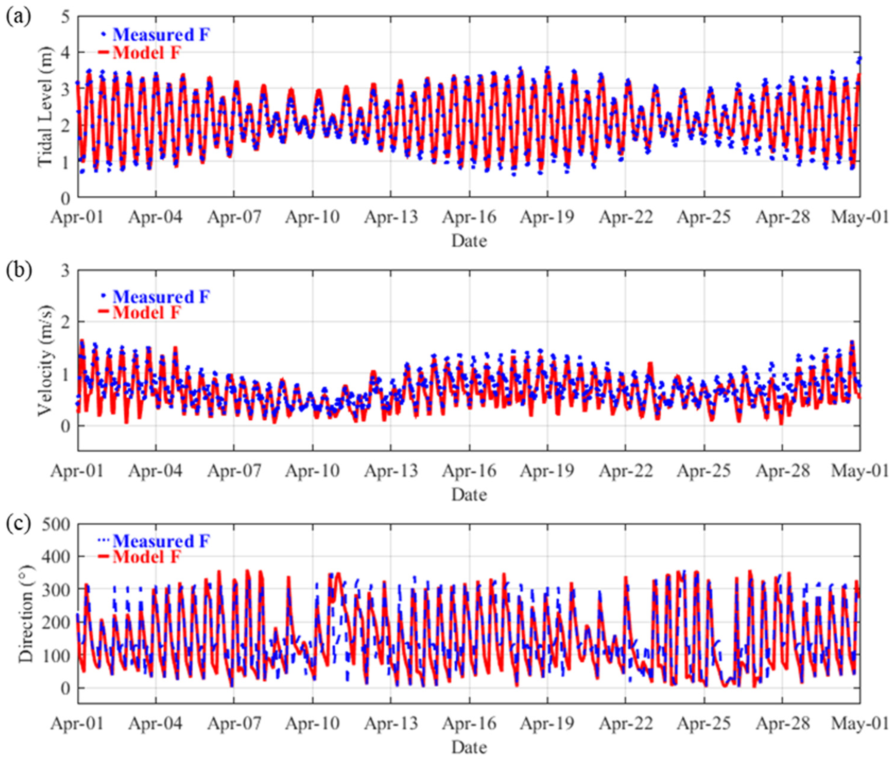
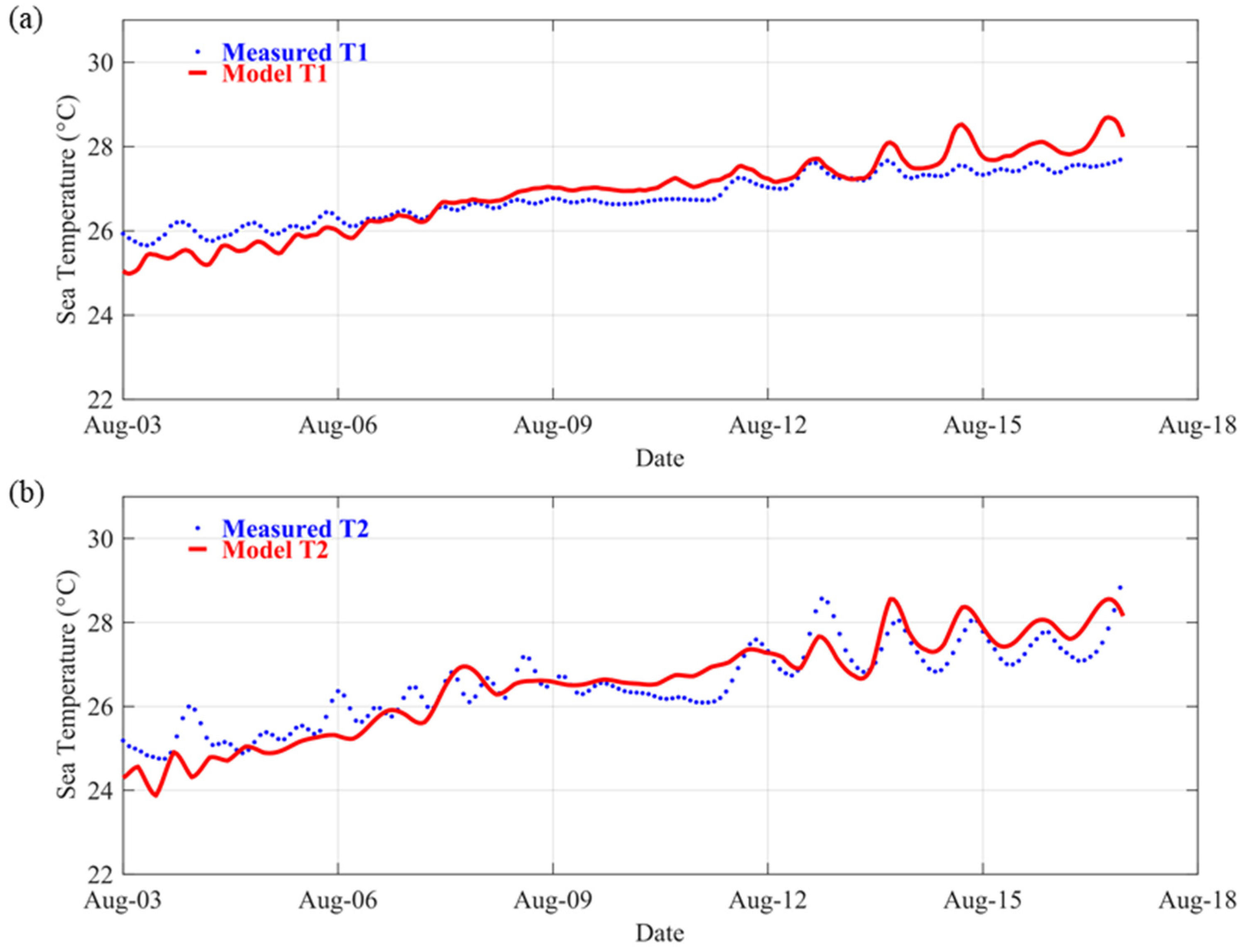
2.2. Model Validation

The observed buoy data obtained at Qushan (marked as the black rectangle in Figure 1, 1–30 April 2018) verified the simulated water level and current, whereas the sea temperature was verified by continuous buoy data obtained at two stations (T1 Daishan, T2 Zhujiajian, marked as the green circle in Figure 1, 3–17 August 2019). The observed buoy data used in this paper were provided by the Marine Monitoring and Forecasting Center of Zhejiang Province. As shown in Figure 2 and Figure 3, the model results well reproduce the magnitudes and trends of the water level, current direction, current velocity and sea temperature. The Root Mean Square Error (RMSE) and Mean Relative Error (MRE) of temperature in T2 are 0.39 °C and 1.24%, respectively. The RMSE and MRE of temperature in T1 are 0.50 °C and 1.53%, respectively. The accuracy of model predictions is validated using a Skill score method [26,27]. The Skill Equation (1) is calculated as follows
S k i l l = 1 i = 1 N | X m o d X o b s | 2 i = 1 N ( | X m o d X ¯ o b s | + | X o b s X ¯ o b s | ) 2
X m o d and X o b s are the simulated values and the measured values, respectively. The Skill is between 0 and 1, which indicates that the measured values are completely consistent (Skill = 1) or inconsistent (Skill = 0) with the simulated values. The Skill score of the water level, current and sea temperature are shown in Table 2. The comparison shows that the ROMS model is accurate.
The results were not only qualitatively analyzed but also quantitatively validated by Equation (2), which calculates the Anomaly Correlation Coefficient (ACC) of the simulated sea surface temperature and the MODIS SST data relative to the climate condition of abnormal, as follows [28]
A C C = i = 1 N { [ ( F i C i ) ( F l C l ) ¯ ] [ ( A i C i ) ( A l C l ¯ ) ] } i = 1 N [ ( F i C i ) ( F l C l ) ¯ ] 2 i = 1 N [ ( A i C i ) ( A l C l ¯ ) ] 2
where F is model data, C is average climatology-state data, A is remote sensing data, over bar is the area mean and i is each grid point in the formula. In general, an ACC value of 0.6 is regarded as the limit for useful validation. The ACC of each month is greater than 0.6, indicating not only the high precision of the simulation but also that the model data can better simulate the difference between SST in 2019 and the annual average SST (Table 3).

2.3. Numerical Tests

The response of the SST distribution, the heating/cooling rate of temperature and temperature fronts in the CR estuary, as well as adjacent waters, to the variations in runoff, has been studied using five numerical experiments (Table 4). In the first comparison experiment, we investigated the effect of CR runoff on the heating and cooling rate of SST in this region by comparing the results of cases of no runoff (case 2), maximum runoff (i.e., the maximum flow in each day between 1999 and 2019, case 3), and the real runoff in 2019, which is shown in Figure 4a (case 1). Note that to ensure model stability, the CR runoff flux is set to less than 20,000 m2/s in case 3 and gradually increases to the maximum within one month. In the second comparison, we investigated the effect of the abundant/scarce runoff conditions (case 4/case 5) on the horizontal and vertical frontal distribution of sea temperature. The scarce situation of annual runoff (the blue dotted line in Figure 4b) and abundant situation of annual runoff (the blue line in Figure 4b) are obtained by modeling average annual flow over two decades and assuming the seasonal variation is the same. Specifically, the flux is calculated through the equation Q = Qi ± (Qmax − Qi) * α. Here Qi and Qmax are the averages and maximum annual flow from 1999 to 2019, respectively, and α is set to 0.25 to investigate an intermediate state. All cases were simulated under the climate forcing (air temperature, air pressure, wind data, relative humidity and radiation flux daily data) and tidal forcing (K1, O1, P1, Q1, M2, S2, N2 and K2) in 2019.

3. Results and Discussion

This section reports the influence of runoff on the heating or cooling rate of SST at first and determines the mechanism of the advection process, which directly effects the upper sea temperature. Secondly, the influence of the scarce or abundant runoff situation on the frontal areas and vertical structure of sea temperature in the CR estuary and its adjacent sea is described and discussed in Section 3.2.

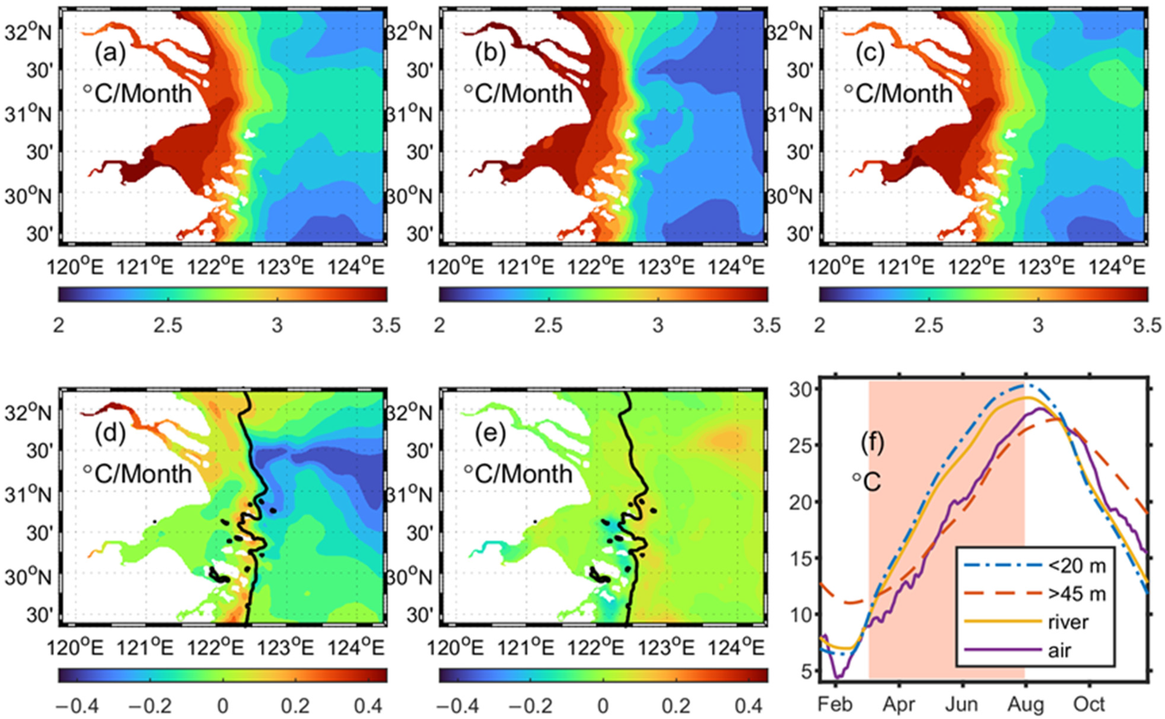
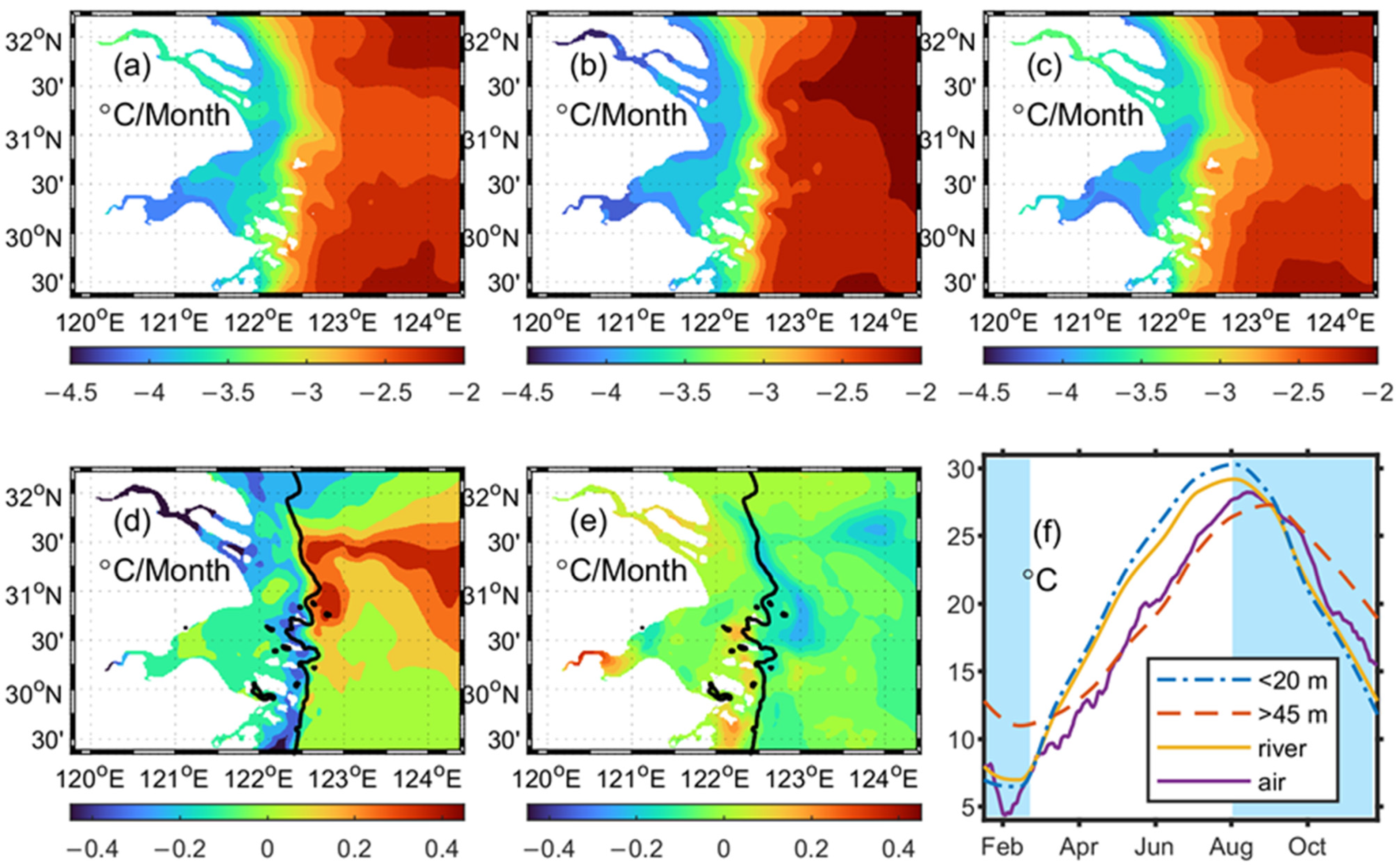
3.1. Influence of CR Runoff on SST

This section analyzes the results of the SST fluctuation rate under the influence of runoff. The distribution patterns of the heating rate in the CR estuary are controlled by seasonal variations in the regional climate and bathymetric effect. In nearshore shallow waters, the SST rises rapidly by 3 °C/month or more, whereas it slowly rises in offshore deep waters by less than 2.5 °C/month (Figure 5a). According to the model results of cases 2 and 3, we calculate the distribution of the heating rate of SST without runoff flux and with maximum runoff flux, respectively (Figure 5b,c). The results show that the distribution patterns of heating rates in these cases follow a similar trend and the heating rate changes dramatically near the large topography gradient (~20 m isobath). When the runoff flux is closed, the heating rate increases by 0.2 °C/month or more near the CR estuary and the Zhoushan archipelago area relative to the actual situation, whereas the heating rate is reduced relative to the actual situation on the east side of the CR estuary where the depth is greater than 20 m, with the maximum reduction close to 0.4 °C/month (Figure 5d). When the maximum runoff flux is used, the heating rate on the east side of the Zhoushan islands where the depth is less than 20 m is reduced by approximately 0.1 °C/month compared to the actual situation, and the heating rate increases outside the CR River estuary where the depth is larger than 20 m with a maximum increment of approximately 0.15 °C/month (Figure 5e).
The above results show that though the spatial distribution patterns of the heating rate are mainly controlled by seasonal variations in the regional climate and bathymetric effect, the runoff flux can generally slow down the heating rate in shallow waters (<20 m) near the CR River estuary and the Zhoushan islands, while having an opposite effect on that in deep waters (>20 m) on the east side of the CR River estuary. The maximum variation in heating rate near a 20 m isobath caused by runoff flux can reach approximately 20% of the total.
With the reduction in daylight and the intensity of solar radiation in the autumn and winter, the SST in this area gradually begins to cool. The terrain effect can cause the temperature in nearshore shallow water to cool rapidly and offshore deep water to cool slowly (Figure 6a). The results of cases 2 and 3 are shown in Figure 6b,c, respectively; the results show that the cooling rate distribution patterns in the three cases are similar to the heating rate distribution patterns. The runoff flux will slow down the cooling rate in shallow waters (<20 m) near the CR River estuary and the Zhoushan islands while having an opposite effect on that in deep waters (>20 m) on the east side of the CR River estuary. The maximum variation in the cooling rate caused by runoff flux can reach approximately 23% of the total.
The heating or cooling rate of the CR estuary and its adjacent sea controlled by runoff flux can be explained by Equation (3) as follows
T t = v T + K s h 2 T + Q net / ρ C p H + Q D
where ρ is the seawater density (=1025 Kg/m3), C p is the specific heat (=3890 J/kg/°C), H is the upper mixed-layer depth, K s h is the eddy diffusive coefficient and v · T is the advection heat transport item. Q n e t and Q D are the net heat flux and vertical heat transport, respectively. Because the K s h 2 T and Q D are the relatively negligible items [10], the heating and cooling rate are mainly due to the effects of dynamics and thermodynamics: the former is the advection process of runoff flow or currents ( v · T ), and the latter is the radiation and conduction process ( Q net / ρ C p ). It is important to note that the local air–sea heat exchange controlled by climate forcing and bathymetric effect determine the seasonal variations in sea temperature in Chinese coastal sea [29]. However, the role of the advection process cannot be neglected in the estuary and its adjacent sea [10], especially in frontal areas with larger T near 20 m.
During the warm season, the heating rate in Hangzhou Bay is the fastest, followed by the CR estuary, and the heating rate in deep waters (>20 m) on the east side of the CR estuary is the slowest (Figure 5f). Among these areas, there is a significant strong front ( T ) near the 20 m isobath. When the v · T controlled by runoff is closed in case 2, the heat of deep waters (>20 m) on the east side of the CR estuary is contributed to only by sea surface heat flux, causing the rate of heating to slow. However, in case 3, the large eastward CR runoff flow transports heat and increases the heating rate. Because of the negative effect of v · T , when the CR runoff flows to shallower and warmer waters, the heating rate will decrease.
During the cooling season, runoff has a similar effect on the cooling rate of the CR estuary. Among these areas, there is also a significant strong front ( T ) near the 20 m isobath. When the v · T controlled by runoff is closed, the heat loss on the deep sea surface (>20 m) on the east side of the CR estuary occurs because the advection process is absent. Therefore, in case 2, the cooling rate will be lower. However, in case 3, the large eastward CR runoff flow transports colder water, increasing the cooling rate. Because of the negative effect of v · T , when the CR runoff flows to shallower and colder waters in winter, the cooling rate will decrease.
The above results show that the runoff flux plays an important role on the temperature frontal areas with larger T . The mechanism of surface and bottom sea temperature variation is different in the deep sea water column of the CR estuary and its adjacent sea due to thermal stratification, except in winter. Therefore, the influence of runoff flux on the sea temperature fronts and vertical structure of sea temperature is described and discussed in Section 3.2.

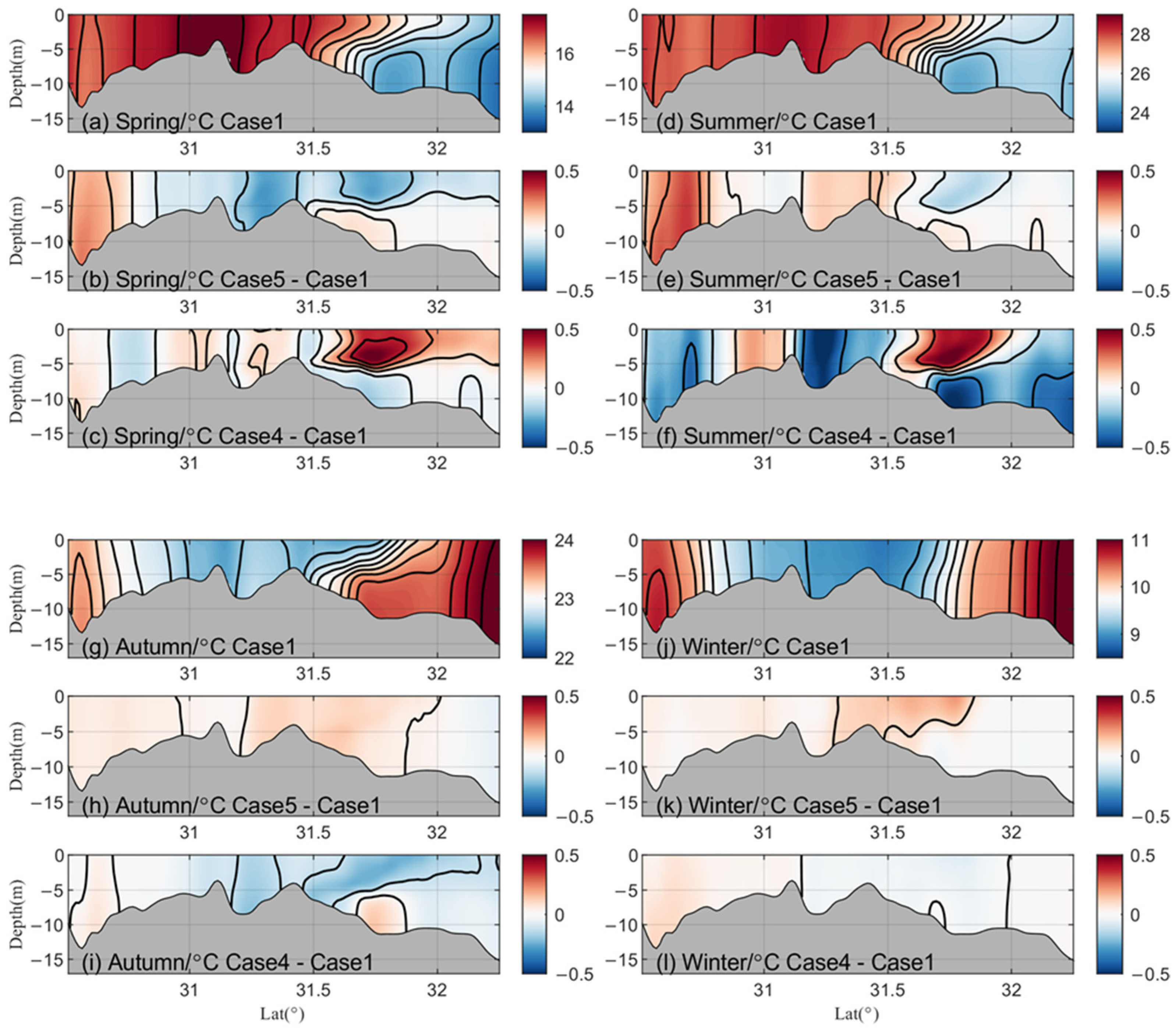
3.2. Influence of CR Runoff on Fronts and Vertical Structure of Sea Temperature

The temperature front in the CR River estuary, which is one of the salient features of its sea temperature distribution structure, has obvious seasonal variation characteristics. It identifies the active area of biogeochemical processes. The effect of runoff in the scarce or abundant situations on the surface and bottom temperature fronts of the CR River estuary are shown in Figure 7 and Figure 8; all of them have obvious seasonal variations. Note that the March–May, June–August, September–November and December–February average data represent spring, summer, autumn and winter results, respectively. The gradient data are calculated in each grid and are time-averaged. The distribution of temperature fronts is dominated by topography and the temperature fronts generally occur in the area with large topography gradient. The effect of the freshwater discharge also plays an important role on the temperature fronts of the upper layer.
In spring (Figure 7a), a strong surface estuary temperature front distributes between the 122° E–122.5° E with magnitudes of approximately 0.06 °C/km near the CR estuary, and approximately 0.1 °C/km near the Zhoushan archipelago area. A weaker surface temperature front with a magnitude of about 0.05 °C/km exists in the middle and south of Hangzhou Bay. As shown in Figure 6b,c, these fronts are stable for their geographical locations, whether the runoff flow is abundant or scarce, but the abundant (scarce) runoff flow can strengthen (weaken) the fronts near the Qushan (marked as the black rectangle in Figure 1). The geographical region of the bottom temperature fronts is similar to that of the surface temperature fronts, but the fronts near the CR estuary in the bottom are stronger than those on the surface (Figure 8a). The abundant runoff flow also can strengthen the bottom fronts; the maximum degree of enhancement at the CR mouth (31.3° N; 122° E) is more than 0.02 °C/km, approximately 45% of the total.
In summer (Figure 7d), the temperature fronts that distribute between 122° E and 122.5° E are the most distinct in the year. The magnitudes of SST gradient near the Zhoushan archipelago area can reach a maximum of approximately 0.1 °C/km, and the fronts near the CR estuary are weaker with a magnitude of approximately 0.05 °C/km. Model results show that the abundant (scarce) runoff flow can strengthen (weaken) the fronts near the Zhoushan archipelago area (Figure 7e,f) with the increments (decrease) of approximately 0.015 °C/km. The maximum degree of enhancement at the northeast of this region (31.5° N; 123.5° E) is more than 0.02 °C/km, approximately 50% of the total (Figure 7d,f). Furthermore, whether the runoff flux remains abundant or scarce, the temperature fronts in Hangzhou Bay will disappear. Meanwhile, the bottom temperature fronts are stronger than the surface as they are not easily influenced by runoff flow, and their coverages are wider than surface temperature fronts in this area where the eastern side of the fronts can reach 123° E.
In autumn (Figure 7g), the temperature of the CR Estuary and Hangzhou Bay area quickly drops and gradually approaches the outer sea temperature (Figure 6f), so the temperature fronts begin to fade, and even disappear in most of the region, and magnitudes of SST gradient fall below 0.04 °C/km. As the temperature gradient decreases (little T ), the value of heat advection decreases accordingly so that the impact of runoff is significantly small. However, there is a significant bottom temperature front near the 123° E from 29.5° N to 31° N in autumn (Figure 8g) because the water still stays cold at the deeper layer due to the strong thermal stratification in summer (Figure 9d). According to previous studies [30], Taiwan’s warm current may reinforce the intensity of this front.
In winter (Figure 7j), with the temperature of the CR estuary and Hangzhou Bay area dropping significantly, fronts start to emerge on the steep slope between 122.5° E and 123° E with magnitudes of approximately 0.05 °C/km. The comparison shows that the abundant runoff flow can strengthen the fronts out of CR near the 123° E (Figure 7l) with increments of approximately 0.015 °C/km or more. The distribution region of the bottom and surface temperature fronts are similar because the water column mixes well in the vertical direction, but the fronts near the CR estuary in the bottom are weaker than those on the surface (Figure 8j). Furthermore, the influence of abundant runoff flow on the bottom fronts is smaller than the surface fronts due to the smaller T .
Based on the influence range of runoff in nearshore shallow and offshore deep waters, two typical sections of 31° N near the CR mouth and 122.2° E located at shallow waters were selected to discuss the impact of the scarce or abundant runoff situation on the vertical distribution and thermal stratification of sea temperature.
As shown in Figure 9 and Figure 10, except in winter, there is a significant thermal stratification on the slope of sections and at the depth of ~20 m. Runoff conditions influence stratification and seasonal variation. In spring, the isotherms of the 31° N section show a relatively uniform vertical distribution pattern below the 20 m layer, where there are vertical fronts in the middle layer at 123° E, indicating that the thermocline is emerging (Figure 9a). The southern part of the 122.2° E section also has a relatively uniform vertical distribution pattern, with a temperature difference of approximately 2 °C near 31.7° N between the bottom and surface (Figure 10a). In the summer, the stratification is significant in both sections of 31° N and 122.2° E, and the result shows that the abundant runoff flux can regulate the vertical variation in these two sections and strengthen the degree of water stratification by warming the upper layer (Figure 9f and Figure 10f), and the water temperature at the deeper layer stays colder close to the value in spring due to the strong thermal stratification. According to Figure 9d–f, the temperature difference is approximately 6 °C in offshore deep waters between the bottom and surface. In the abundant runoff flux case, the difference increases to 8 °C, while the difference decreases to approximately 5 °C with scarce runoff flux.
In autumn, the stratification near the slope disappears, while at the depth of ~30 m it remains visible. The influence of runoff flux on the upper layer becomes weaker because of the little T . However, the water at the deeper layer remains colder due to the strong thermal stratification in summer caused by runoff flux, resulting in the vertical temperature front (Figure 9g). In the scarce runoff flux case, the temperature difference is approximately 1 °C in offshore deep waters between the bottom and surface (Figure 9h), while the difference increases by 2 °C with abundant runoff flux. The influence of CR runoff on the vertical structure of sea temperature at nearshore shallow waters is weaker due to weaker thermal stratification at the section of 122.2° N in the autumn (Figure 10h). In the winter, the water column mixed well in the vertical direction due to the sea surface cooling sharply, controlled by atmospheric forcing of the region. As a result, the phenomenon of stratification is absent, and the influence of CR runoff on the vertical structure of sea temperature can be neglected (Figure 9j and Figure 10j). The horizontal temperature gradient remains in the sections mainly dominated by bathymetric effect. Under abundant runoff regulation, the horizontal temperature gradient is smaller at the east area of 123.5° E.

4. Conclusions

In this study, we discuss the impact of river discharges on the sea temperature structure in the CR estuary and its adjacent sea. The change in runoff flow has a considerable influence on advection heat transport ( v · T ). As the volume of runoff increases, the variations in the heating or cooling rate begin to be regulated because of the temperature difference between shallow and deep areas. During the warm season, there is a significant strong front (∇T) near the 20 m isobath among these areas. When the runoff controlled −v·∇T is closed, the heat of deep waters (>20 m) on the east side of the CR estuary is contributed to only by sea surface heat flux, causing the rate of heating to slow. However, in case 3, the large eastward CR runoff flow transports heat and increases the heating rate. Because of the negative effect of v · T , when the CR runoff flows to shallower and warmer waters, the heating rate decreases. During the cooling season, runoff has a similar effect on the CR estuary’s cooling rate. In the absence of a river, the cooling rate will be lower on the sea deeper than 20 m, and it will be higher in the maximum runoff condition. In winter, the CR runoff flows to shallower and colder waters.
In all three cases (natural, abundant or scarce runoff conditions), a strong surface estuary temperature front distributes between 122° E and 122.5° E. The results show a positive correlation between runoff conditions and the intensity of the horizon frontal zones in the CR estuary. The effect of the freshwater discharge on the surface layer is greater than that on the bottom layer. The effect of CR runoff on the temperature front varies significantly seasonally. Because of the smallest ∇T, the effect in autumn is the weakest. The abundant runoff can regulate the vertical variation of seawater and strengthen the water stratification.
Although the present model provides a framework to understand and evaluate the impacts of river discharge on sea temperature, there is still a knowledge gap in coastal dynamics and the accuracy of model predictions due to a lack of observation of the changing ocean. The number of observation buoys and satellites has never been sufficient to monitor the variability in the temperature structure over the entire region where the CDW influences the water masses. Therefore, conducting multi-platform four-dimensional (latitude, longitude, depth, time) observational surveys with efficient means (assimilation system) in the CR estuary and its adjacent sea, focusing on the thermohaline structure at a large spatio-temporal scale, would be helpful to conduct.

Author Contributions

Conceptualization, H.S.; Data curation, H.S. and Y.Z.; Funding acquisition, Y.Z.; Methodology, H.S. and Y.L.; Project administration, Z.H.; Validation, L.L.; Visualization, H.S.; Writing—original draft, H.S.; Writing—review & editing, Y.Z., Z.H., L.L. and Y.L. All authors have read and agreed to the published version of the manuscript.

Funding

This study was supported by the NSFC-Zhejiang Joint Fund for the Integration of Industrialization and Informatization (U1709204), and the National Key Research and Development Program of China (Grant No. 2016YFC1400100, 2017YFC0305905).

Institutional Review Board Statement

Not applicable.

Informed Consent Statement

Not applicable.

Data Availability Statement

We are grateful for the NCEP-DOE Reanalysis 2, JCOPE2 (Japan Coastal Ocean Predictability Experiments 2), global tidal model TPXO and the MODIS remote sensing products. We are also grateful for Datong hydrological station, Fuchunjiang hydrology station and Marine Monitoring and Forecasting Center of Zhejiang Province to provide the river discharge data and the observed buoy data.

Acknowledgments

We would like to thank A.P. Shuangyan He for their valuable comments.

Conflicts of Interest

The authors declare no conflict of interest.

References

  1. Beardsley, R.; Limeburner, R.; Yu, H.; Cannon, G. Discharge of the Changjiang (Yangtze river) into the East China sea. Cont. Shelf Res. 1985, 4, 57–76. [Google Scholar] [CrossRef]
  2. Su, J.; Kangshan, W. Changjiang river plume and suspended sediment transport in Hangzhou Bay. Cont. Shelf Res. 1989, 9, 93–111. [Google Scholar]
  3. Liu, X.; Hou, Y.; Yin, B.; Yang, D. Dynamics of circulation and temperature-salinity structures in Changjiang river mouth and its adjacent sea: III. The temperature structure. Chin. J. Oceanol. Limnol. 2015, 46, 526–533. [Google Scholar]
  4. Chen, C.; Beardsley, R.; Limeburner, R.; Kim, K. Comparison of winter and summer hydrographic observations in the Yellow and East China Seas and adjacent Kuroshio during 1986. Cont. Shelf Res. 1994, 14, 909–929. [Google Scholar] [CrossRef]
  5. Chang, P.; Isobe, A. A numerical study on the Changjiang diluted water in the Yellow and East China Seas. J. Geophys. Res. Oceans 2003, 108, 3299. [Google Scholar] [CrossRef]
  6. Zeng, X.; He, R.; Zong, H. Variability of Changjiang Diluted Water revealed by a 45-year long-term ocean hindcast and Self-Organizing Maps analysis. Cont. Shelf Res. 2017, 146, 37–46. [Google Scholar] [CrossRef]
  7. Bai, Y.; He, X.; Pan, D.; Chen, C.; Kang, Y.; Chen, X.; Cai, W. Summertime Changjiang River plume variation during 1998–2010. J. Geophys. Res. Oceans 2014, 119, 6238–6257. [Google Scholar] [CrossRef]
  8. Chen, C.; Xue, P.; Ding, P.; Beardsley, R.; Xu, Q.; Mao, X.; Gao, G.; Qi, J.; Li, C.; Lin, H. Physical mechanisms for the offshore detachment of the Changjiang Diluted Water in the East China Sea. J. Geophys. Res. Oceans 2008, 113, C02002. [Google Scholar] [CrossRef]
  9. Wang, Y.; Shen, J.; He, Q.; Zhu, L.; Zhang, D. Seasonal variations of transport time of freshwater exchanges between Changjiang Estuary and its adjacent regions. Estuar. Coast. Shelf Sci. 2015, 157, 109–119. [Google Scholar] [CrossRef]
  10. Huang, D.; Zhang, T.; Zhou, F. Sea-surface temperature fronts in the Yellow and East China Seas from TRMM microwave imager data. Deep Sea Res. Part II 2010, 57, 1017–1024. [Google Scholar] [CrossRef]
  11. Wang, B. Hydromorphological mechanisms leading to hypoxia off the Changjiang estuary. Mar. Environ. Res. 2009, 67, 53–58. [Google Scholar] [CrossRef] [PubMed] [Green Version]
  12. Zhou, F.; Xuan, J.; Ni, X.; Huang, D. A preliminary study of variations of the Changjiang Diluted Water between August of 1999 and 2006. Acta Oceanol. Sin. 2009, 28, 1–11. [Google Scholar]
  13. Moon, J.; Pang, I.; Yoon, J. Response of the Changjiang diluted water around Jeju Island to external forcings: A modeling study of 2002 and 2006. Cont. Shelf Res. 2009, 29, 1549–1564. [Google Scholar] [CrossRef]
  14. Sukigara, C.; Mino, Y.; Tripathy, S.; Ishizaka, J.; Matsuno, T. Impacts of the Changjiang diluted water on sinking processes of particulate organic matters in the East China Sea. Cont. Shelf Res. 2017, 151, 84–93. [Google Scholar] [CrossRef]
  15. Xu, Y.; Cai, Y.; Sun, T.; Xu, W.; Yang, Z. Impacts of Temperature Gradient on the Intensity of Physical Disturbance and the Water Ecological Biodiversity in the River Estuary. Int. J. Environ. Sci. Technol. 2016, 7, 595–600. [Google Scholar] [CrossRef] [Green Version]
  16. Wu, H.; Wu, T.; Bai, M. Mega Estuarine Constructions Modulate the Changjiang River Plume Extension in Adjacent Seas. Estuaries Coasts 2018, 41, 1234–1252. [Google Scholar] [CrossRef]
  17. Hornerdevine, A.; Hetland, R.; Macdonald, D. Mixing and Transport in Coastal River Plumes. Annu. Rev. Fluid Mech. 2015, 47, 569–594. [Google Scholar] [CrossRef]
  18. Simpson, J.; Hunter, J. Fronts in the Irish sea. Nature 1974, 250, 404–406. [Google Scholar] [CrossRef]
  19. Qiu, C.; Zhu, J. Influence of seasonal runoff regulation by the Three Gorges Reservoir on saltwater intrusion in the Changjiang River Estuary. Cont. Shelf Res. 2013, 71, 16–26. [Google Scholar] [CrossRef]
  20. Herb, W.; Stefan, H. Modified equilibrium temperature models for cold-water streams. Water Resour. Res. 2011, 47, W06519. [Google Scholar] [CrossRef] [Green Version]
  21. Haidvogel, D.; Arango, H.; Hedstrom, K.; Beckmann, A.; Malanotte-Rizzoli, P.; Shchepetkin, A. Model evaluation experiments in the North Atlantic Basin: Simulations in nonlinear terrain-following coordinates. Dyn. Atmos. Oceans 2000, 32, 239–281. [Google Scholar] [CrossRef]
  22. Di-Lorenzo, E. Seasonal dynamics of the surface circulation in the southern California Current System. Deep Sea Res. Part II 2003, 50, 2371–2388. [Google Scholar] [CrossRef]
  23. Wilkin, J.; Arango, H.; Haidvogel, D.; Lichtenwalner, C.; Durski, S.; Hedstrom, K. A regional Ocean Modeling System for the Long-term Ecosystem Observatory. J. Geophys. Res. 2005, 110, C06S91. [Google Scholar] [CrossRef] [Green Version]
  24. Yuan, D.; Zhu, J.; Li, C.; Hu, D. Cross-shelf circulation in the Yellow and East China Seas indicated by MODIS satellite observations. J. Marine Syst. 2008, 70, 134–149. [Google Scholar] [CrossRef]
  25. Pawlowicz, R.; Beardsley, B.; Lentz, S. Classical tidal harmonic analysis including error estimates in MATLAB using T_TIDE. Comput. Geosci. 2002, 28, 929–937. [Google Scholar] [CrossRef]
  26. Willmott, C. On the validation of models. Phys. Geogr. 1981, 2, 184–194. [Google Scholar] [CrossRef]
  27. Warner, J.; Geyer, W.; Lerczak, J. Numerical modeling of an estuary: A comprehensive skill assessment. J. Geophys. Res. Oceans 2005, 110, C5. [Google Scholar] [CrossRef]
  28. Krishnamurti, T.; Rajendran, K.; Vijaya Kumar, T.; Lord, S.; Toth, Z.; Zou, X.; Cocke, S.; Ahlquist, J.E.; Navon, I.M. Improved skill for the anomaly correlation of geopotential heights at 500 hPa, Mon. Weather Rev. 2003, 131, 1082–1102. [Google Scholar] [CrossRef] [Green Version]
  29. Xie, S.; Hafner, J.; Tanimoto, Y.; Liu, W.; Tokinaga, H.; Xu, H. Bathymetric effect on the winter sea surface temperature and climate of the Yellow and East China Seas. Geophys. Res. Lett. 2002, 29, 2228. [Google Scholar] [CrossRef] [Green Version]
  30. Zhang, Q.; Liu, H.; Qin, S.; Yang, D.; Liu, Z. The study on seasonal characteristics of water masses in the western East China Sea shelf area. Acta Oceanol. Sin. 2014, 33, 54–74. [Google Scholar] [CrossRef]
Figure 1. The topography (m) of the CR estuary and adjacent waters. F station is for water level and current. T1 and T2 stations are for sea temperature.
Jmse 10 00343 g001
Figure 2. Verification of (a) water level, (b) current velocity and (c) direction (1–30 April 2018).
Jmse 10 00343 g002
Figure 3. Verification of sea temperature in (a) T1 and (b) T2 (3–17 August 2019).
Jmse 10 00343 g003
Figure 4. The runoff volume set in (a) case 1—2019, (b) case 4—abundant and case 5—scarce.
Jmse 10 00343 g004
Figure 5. The effect of the runoff on the heating rate of surface temperature during the warm season. (a) with real runoff flux in 2019, (b) without runoff flux, (c) with maximum runoff flux, (d) b minus a, (e) c minus a (the black lines indicate 20 m isobath), (f) the variation in the nearshore shallow sea temperature, offshore deep sea temperature, CR inflow temperature and air temperature near sea surface, the red shaded areas indicate the warm season.
Jmse 10 00343 g005
Figure 6. The effect of runoff on the cooling rate of surface temperature during the cooling season. (a) with real runoff flux in 2019, (b) without runoff flux, (c) with maximum runoff flux, (d) b minus a, (e) c minus a (the black lines indicate 20 m isobath), (f) the variation in the nearshore shallow sea temperature, offshore deep sea temperature, CR inflow temperature and air temperature near sea surface, the blue shaded areas indicate the cooling season.
Jmse 10 00343 g006
Figure 7. Influence of scarce or abundant situation of runoff on surface fronts. (a,d,g,j) (case 1 results in Spring, Summer, Autumn and Winter); (b,e,h,k) (the difference between case 1 and case 5 in Spring, Summer, Autumn and Winter); (c,f,i,l) (the difference between case 1 and case 4 in Spring, Summer, Autumn and Winter).
Jmse 10 00343 g007
Figure 8. Influence of scarce or abundant situation of runoff on bottom fronts. (a,d,g,j) (case 1 results in Spring, Summer, Autumn and Winter); (b,e,h,k) (the difference between case 1 and case 5 in Spring, Summer, Autumn and Winter); (c,f,i,l) (the difference between case 1 and case 4 in Spring, Summer, Autumn and Winter).
Jmse 10 00343 g008
Figure 9. The sectional distribution of sea temperature (°C, 31° N). (a,d,g,j) (case 1 results in Spring, Summer, Autumn and Winter); (b,e,h,k) (the difference between case 1 and case 5 in Spring, Summer, Autumn and Winter); (c,f,i,l) (the difference between case 1 and case 4 in Spring, Summer, Autumn and Winter).
Jmse 10 00343 g009
Figure 10. The sectional distribution of sea temperature (°C, 122.2° N). (a,d,g,j) (case 1 results in Spring, Summer, Autumn and Winter); (b,e,h,k) (the difference between case 1 and case 5 in Spring, Summer, Autumn and Winter); (c,f,i,l) (the difference between case 1 and case 4 in Spring, Summer, Autumn and Winter).
Jmse 10 00343 g010
Table 1. Model configuration.
Model ParametersParameter Configuration
Model domain29°–32.5° N, 120°–124°30′ E
Grid resolution50″ × 50″ in each horizontal direction,
20 sigma layer, θs 7.0, θb 2.0, the minimum depth 3 m
Initial conditionswater level, current and sea surface level were 0, temperature and salinity were interpolated from HYCOM
Boundary conditionsDatong, Fuchunjiang hydrology station as two points source in the lateral boundary; Tidal forcing K1, O1, P1, Q1, M2, S2, N2, K2
Climate DataOpen boundary: temperature and salinity from JCOPE2Air temperature, air pressure, wind data, relative humidity and radiation flux used NOAA-released NCEP/NCAR reanalysis data.
Table 2. The Skill score of water level, current direction, current velocity and sea temperature.
Water LevelCurrent VelocityCurrent DirectionSea Temperature
Skill0.9810.9010.9220.929/0.932
Table 3. Verification of calculated results of SST–ACC value (January–December).
JanuaryFebruaryMarchAprilMayJune
0.6130.7120.7880.8280.6170.737
JulyAugustSeptemberOctoberNovemberDecember
0.7890.7960.7660.6840.7580.769
Table 4. Descriptions of numerical tests.
TestCRQTRTidal ForcingClimate Forcing
Case 12019201920192019
Case 2Off201920192019
Case 3Maximum201920192019
Case 4Abundant201920192019
Case 5Scare201920192019
Publisher’s Note: MDPI stays neutral with regard to jurisdictional claims in published maps and institutional affiliations.

