Article

Effects of Miniaturization of the Summer Phytoplankton Community on the Marine Ecosystem in the Northern East China Sea

1
Oceanic Climate & Ecology Research Division, National Institute of Fisheries Science, Busan 46083, Korea
2
HAERANG Technology and Policy Research Institute, Suwon 16229, Korea
*
Author to whom correspondence should be addressed.
J. Mar. Sci. Eng. 2022, 10(3), 315; https://doi.org/10.3390/jmse10030315
Submission received: 25 January 2022 / Revised: 14 February 2022 / Accepted: 20 February 2022 / Published: 23 February 2022

Abstract

:
After the construction of the Three Gorges Dam (Changjiang River), the northern East China Sea has been exposed to major environmental changes in the summer due to climate change and freshwater control. However, little is known regarding phytoplankton in this area. Here, we investigated differences in the summer phytoplankton-community structure as a consequence of marine-environment changes from 2016 to 2020. In the 2000s, the key dominant species in the summer phytoplankton community in the northern East China Sea were diatoms and dinoflagellates. In this study, however, nanoflagellates of ≤20 µm were identified as the dominant species throughout the survey period, with abundances ranging from 43.1 to 69.7%. This change in the phytoplankton-community structure may be ascribed to low nutrient concentrations in the area, especially phosphate, which was below the detection limit, seriously hampering phytoplankton growth. The relative contribution of picophytoplankton to the total chlorophyll a biomass was highest in the surface mixed layer with low nutrient concentrations. Spatially, higher percentages were observed along the east-side stations than the west-side stations, where nutrient concentrations were relatively high. Conclusively, decreased nutrients led to phytoplankton miniaturization. Accordingly, as the dominance of picophytoplankton increases, energy transfer is expected to decrease at the upper trophic level.

1. Introduction

The northern East China Sea is exposed to various currents depending on the season and exhibits singular seasonal fluctuations [1]. It is known to be a highly valuable fishing ground because of its high primary productivity [2,3,4]. In summer, in particular, it shows diverse water mass characteristics, with the surface layer affected by the freshwater flowing in from the coastal areas of China, the bottom layer affected by the cold deep water of the Yellow Sea, and the eastern part affected by the high temperature and salinity of the Kuroshio water. The fronts formed at the boundaries of water masses with different characteristics show unique biological and chemical patterns and have significant effects on the distribution of zooplankton and fish along the food chain [5]. The inflow of freshwater due to Changjiang diluted water shows marked seasonal variability, with the minimum discharge in the winter and the maximum discharge in the summer, which greatly affects the seasonal salinity distribution in the northern East China Sea [6,7]. Moreover, as a major nutrient source [8], the coastal waters of China that are adjacent to the Changjiang are rich in nutrients, with high primary productivity [9,10,11] and characteristics of an estuary dominated by Chinese coastal waters. Geographically, a large difference in water depths is observed between the eastern and western waters, and complex topographical characteristics and diverse water masses show complex environmental interactions with seasonally variable intensity. Thus, the East China Sea, which is characterized by high productivity, is used jointly by Korea, Japan, and China as the largest fishing ground for migratory fish species [3]. Studies on phytoplankton distributions in the East China Sea were mainly conducted by Chinese and Japanese researchers in the 1980s and 1990s [12,13,14,15,16,17,18]. The focus areas of phytoplankton abundances and chlorophyll a (chl-a) concentrations were high in the waters affected by the Changjiang dilution water in spring and autumn [4], changes in phytoplankton standing stocks due to the stratification of the bottom layer structure in summer [19], the relationship between phytoplankton-community structures and water masses in summer [20,21], zooplankton (phytoplankton predators) [22,23,24,25], and changes in chl-a concentrations related to nutrients and suspended matter along with changes in phytoplankton-community structures [26]. In Korea, studies have been conducted on the changes in phytoplankton-community distributions and structures [27,28,29,30] since the 1990s. Several studies have been conducted on different topics, including the distribution characteristics of chl-a according to summer nutrients and suspended substances [31,32] and long-term changes in surface water temperatures and chl-a biomasses [33]. It was also reported that the primary productivity decreased by approximately 86% in waters adjacent to the Changjiang River after the construction of the Three Gorges Dam and that the phytoplankton-community structure in the East China Sea changed [34,35]. However, there appears to be a lack of recent data on this subject matter. Phytoplankton communities in marine ecosystems are sensitive to environmental changes, resulting in noticeable changes in community compositions and standing stocks following changes in physical- and chemical-environmental factors. Therefore, these changes in the phytoplankton-community structure can be used as an indicator of changes in the marine ecosystem. Moreover, in order to properly understand the structure and function of a marine ecosystem, it is necessary to understand temporal and spatial changes that occur in the phytoplankton-community structure in response to environmental factors [36]. The results of this study and those of previous studies were compared to confirm the change in the marine environment in the northern East China Sea due to the effect of constructing the Three Gorges Dam and the effects on the pelagic ecosystems according to the changes in the phytoplankton community structure were investigated.

2. Materials and Methods

2.1. Cruises and Sampling

To determine the distribution profiles of summer phytoplankton communities in the northern East China Sea, we conducted five field surveys from 2016 to 2020 (23 August–6 September 2016; 27 August–6 September 2017; 2–10 August 2018; 20–30 August 2019; and 3–15 August 2020) at the study site. The study site covered three lines and 15 sampling stations, and the surveys were conducted using the ocean research vessel, Tamgu 3 (797 tons; National Institute of Fisheries Sciences), as indicated in Figure 1 and Table 1. For nutrient analysis and quantitative analysis of phytoplankton, we collected samples at seven maximum water depths (0, 10, 20, 30, 50, 75, and 100 m) using Niskin bottles (8 L polyvinyl chloride) attached to a CTD/rosette sampler. The vertical distributions of water temperatures and salinities were measured using a calibrated SBE 9/11 CTD instrument (Sea-Bird Electronics, Bellevue, WA, USA), where descending data were used for the CTD data analysis.

2.2. Dissolved Inorganic Nutrients

For nutrient analysis, we filtered seawater samples (10 mL) through 0.45 µm disposable membrane filter units (Advantec, Tokyo, Japan), placed the samples in conical tubes (15 mL), washed them with hydrochloric acid (HCl, 10%), and immediately stored them at −20 °C. After thawing the samples at room temperature (20 ± 2 °C), we analyzed the ammonium (NH4), nitrite (NO2), nitrate (NO3), phosphate (PO4), and silicon dioxide (SiO2) concentrations with an automatic nutrient analyzer (Quaatro, Seal Analytical, Norderstedt, Germany). The sum of the NH4, NO2, and NO3 concentrations was calculated as the dissolved inorganic nitrogen (DIN).

2.3. Phytoplankton Abundances and Dominant Species

For quantitative analysis of phytoplankton, each sample was collected in a 1 L square PE bottle at a standard water depth at each sampling station, fixed with Lugol’s solution (diluted to a final concentration of 1%), and transported to our laboratory. After 48 h decantation, the lower layer (200 mL) containing the sedimented algae was put in a small measuring cylinder. After being allowed 48 h for decantation, the lower layer (20 mL) containing the sedimented algae was put in a glass vial and stored in a dark box. The concentrated samples were observed under an optical microscope (Nikon eclipse, Ni-U, Nikon Imaging Japan Inc., Tokyo, Japan) at 100× to 1000× magnification, using a Sedwick–Rafter Chamber for species identification and counting [37,38,39,40]. The resulting data were converted to the number of cells·L−1, and species accounting for >5% of the total standing stock were classified as dominant species.

2.4. Picophytoplankton Abundances

To prepare picophytoplankton samples, collected seawater was filtered through a 3 µm polycarbonate membrane filter (Whatman, Florham Park, NJ, USA), split into 5 mL aliquots, and placed in cryogenic tubes. Glutaraldehyde was added to each tube at a final concentration of 1% and allowed to settle for 15 min at room temperature. The samples were then stored at −80 °C. To prepare the samples for picophytoplankton counting, they were thawed shortly before analysis and mixed with yellow-green fluorescent microspheres (0.5 µm diameter beads; Polysciences, Inc., Warrington, PA, USA), an internal reference material for standardizing scattering and fluorescence. Counting was conducted using a flow cytometer equipped with a 488 nm (1 W) argon ion laser (NovoCyte 2060R, ACEA Biosciences Inc., San Diego, CA, USA; BD AccuriTM C6 Plus, BD Biosciences Inc., Franklin Lakes, NJ, USA) (Figure 2), and each picophytoplankton group was distinguished based on the characteristic side scattering of red fluorescence at a 90°-angle, the chl-a concentration, and the orange fluorescence from phycoerythrin (Figure 2). The flow cytometry data were analyzed using NovoExpress (Ver. 1.2.5, ACEA Biosciences Inc., San Diego, CA, USA) and BD AccuriTM C6 Plus Analysis Software (Ver. 1.0.23.1, BD Biosciences Inc., Franklin Lakes, NJ, USA).

2.5. Chl-a Size Fractionation

Chl-a concentrations were calculated as previously described [41]. To measure chl-a concentrations according to the phytoplankton size (>20 µm: micro; 20 µm ≥ chl-a > 3 µm: nano; ≤3 µm: pico), each phytoplankton sample (0.5 L) was sequentially filtered through a 20 µm membrane (Polycarbonate Track Etched Membrane disk, 47 mm diameter, GVS, Sanford, ME, USA), a 3 µm polycarbonate membrane filter (47 mm diameter, Whatman, Florham Park, NJ, USA), and a 0.45 µm membrane filter (47 mm diameter, ADVANTEC, Tokyo, Japan) and mounted on the filter holders. After measuring the chl-a concentrations in the microphytoplankton, nanophytoplankton, and picophytoplankton, the total chl-a concentration was calculated by addition. All filters were transferred to our lab in frozen storage (−80 °C), and chl-a was extracted after solvation in 90% acetone and settling in a dark and cool chamber for 24 h. The extract was then filtered through a 0.45 µm syringe filter (PTFE, Advantec, Florham Park, NJ, USA) to remove particulate matter. Finally, the absorbance values were measured using a 10-Au field fluorometer (Tuner Designs, San Jose, CA, USA) calibrated with standard chl-a (Sigma-Aldrich, Darmstadt, Germany).

2.6. Data Analyses

The R statistical program (Ver. 4.0.3) was used to analyze statistical correlations between environmental factors and phytoplankton groups collected in the northern East China Sea. First, the decorana function of the vegan package of R was used to examine the distributions of biological parameters, which revealed that the DCA1 axis length (1.6993) was less than 3. Accordingly, a redundancy analysis (RDA) was performed.

3. Results

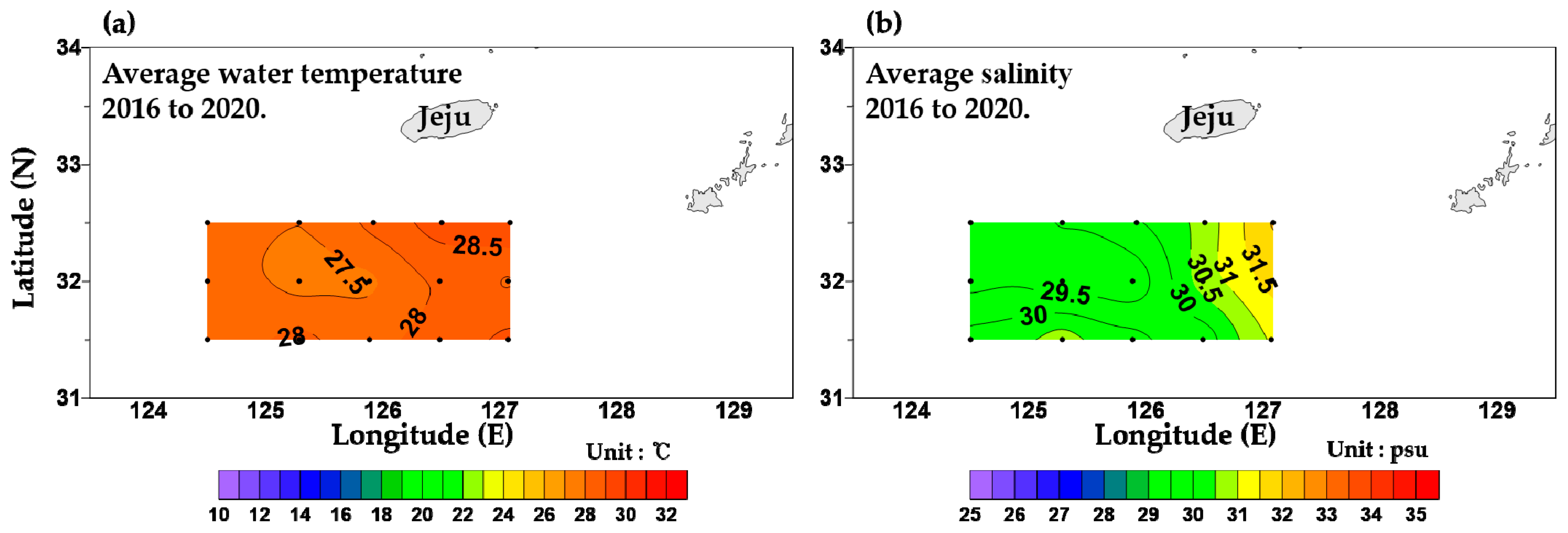
3.1. Physical Environments

Figure 3 and Figure 4 show plots of the surface and vertical profiles of the mean water temperature and salinity in the northern East China Sea. The average surface water temperature in August ranged from 27.3 to 28.9 °C, with an overall average of 28.0 ± 0.5 °C and no distinctive spatial-distribution profile (Figure 3, left). The distribution range of surface salinity was 29.1–32.1, with an average of 30.2 ± 0.9 and a low-west and high-east distribution profile (Figure 3, right). The average vertical water temperature ranged from 15.1 to 28.9 °C, with an overall average of 22.6 ± 4.8 °C, and revealed that a strong thermocline formed at a depth of 20–30 m (Figure 4, top). The average salinity ranged from 29.1 to 34.5 psu, with an overall average of 32.0 ± 1.6 psu (Figure 4, bottom). The western part of the sea had a low salinity (≤31.0 psu from the surface layer to a depth of 20 m), reflecting the influence of the Changjiang dilution water. The deep layer of the eastern part of the sea had a high salinity of ≥34.0 psu, reflecting the influence of the Kuroshio water. In August, the northern East China Sea formed a complex water mass structure under the influence of various water masses, depending on the water depths between the sampling stations.

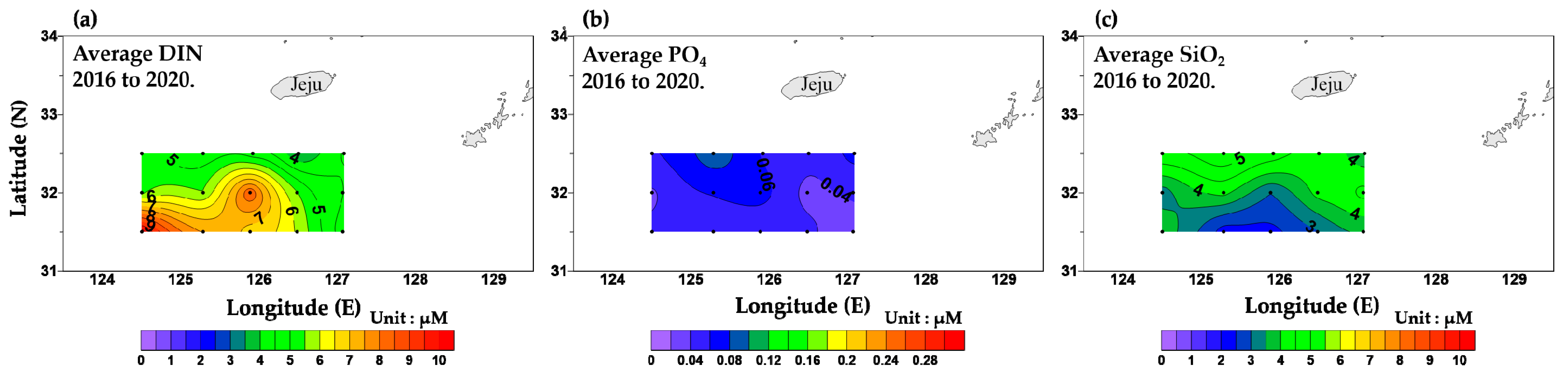
3.2. Dissolved Inorganic Nutrient Concentrations

The average surface-layer DIN, PO4, and SiO2 concentrations in the northern East China Sea in August were 3.5–10.3 μM, <0.1–0.1 μM, and 2.2–5.5 μM, respectively (Figure 5). The DIN concentration increased from north to south, while the PO4 and SiO2 concentrations showed a spatial-distribution profile with a gradual decrease from north to south. The average vertical DIN, PO4, and SiO2 concentration ranges were 2.5–19.5 μM, <0.1–0.8 μM, and 2.5–19.5 μM, respectively (Figure 6). Throughout the survey period, the DIN tended to increase from the surface to the bottom layer, and the PO4 concentration was extremely low in the surface mixed layer, at the detection limit of ≤0.1 μM.

3.3. Phytoplankton Abundance and Dominant Species

In the summer, the average phytoplankton standing stock at the depth of each station ranged from 7955 to 1,090,202 cells·L−1, with an overall average count of 149,656 ± 192,162 cells·L−1. Spatially, in the western part of the sea (affected by the Changjiang River dilution water), the standing stock was approximately three times higher than that in the eastern part of the sea (affected by offshore waters). Due to strong vertical stratification in the summer, over 90% of the total standing stock appeared in the surface mixed layer (water depth: 0–30 m), demonstrating a remarkable difference between the surface and bottom layers. Nanoflagellates (≤20 μm) appeared to be the dominant species throughout the survey period. Moreover, with Scrippsiella acuminata (which inhabits the coastal environment) reaching a high abundance in the western part of the sea, flagellates predominated in summer. In addition, at specific times during the survey, diatoms such as Chaetoceros lorenzianus, Guinardia flaccida, Paralia sulcate, and Thalassiosira spp., and dinoflagellates such as Alexandrium spp. appeared as the dominant species (Table 2).

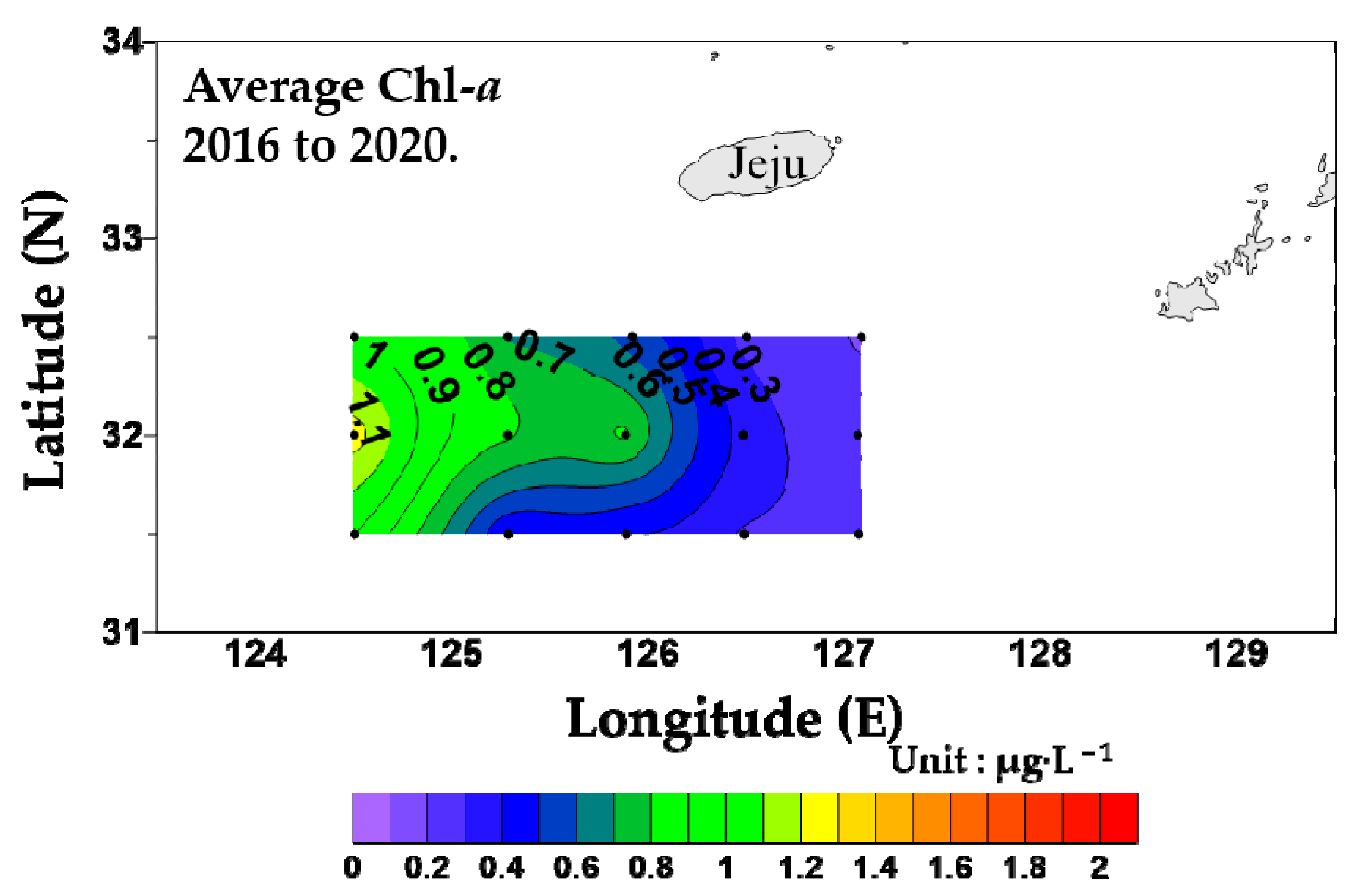
3.4. Relative Contributions of Size-Fractionated Chl-a to the Overall Chl-a Concentration

The average surface-layer concentration of chl-a in the northern East China Sea in summer ranged from 0.19 to 1.25 µg·L−1, with an overall average of 0.57 ± 0.33 µg·L−1 that gradually decreased going from west to east (Figure 7). The vertical distribution of chl-a ranged from 0.04 to 1.99 µg·L−1 with an overall average of 0.52 ± 0.40 µg·L−1, where the distribution was higher in the surface mixed layer along the thermocline and gradually decreased going toward the bottom. In addition, the subsurface chl-a maximum layer developed at a depth of 10 to 20 m in the western part of the sea, and at 20 to 30 m in the eastern part, depending on the locations of the sampling stations (Figure 8).
The average relative contributions of microphytoplankton, nano phytoplankton, and picophytoplankton to the chl-a concentrations were 2.9–54.1% (23.2 ± 11.9%), 13.7–59.9% (28.7 ± 12.6%), and 16.4–770% (48.1 ± 16.2%), respectively. Spatially, microphytoplankton contributed more to the chl-a concentration in the western part of the sea, and picophytoplankton contributed more in the eastern part of the sea, showing opposite spatial distributions. Vertically, the relative contributions of microphytoplankton and nanophytoplankton increased from the surface layer to the bottom layer, whereas that of the picophytoplankton tended to decrease toward the bottom layer (Table 3).

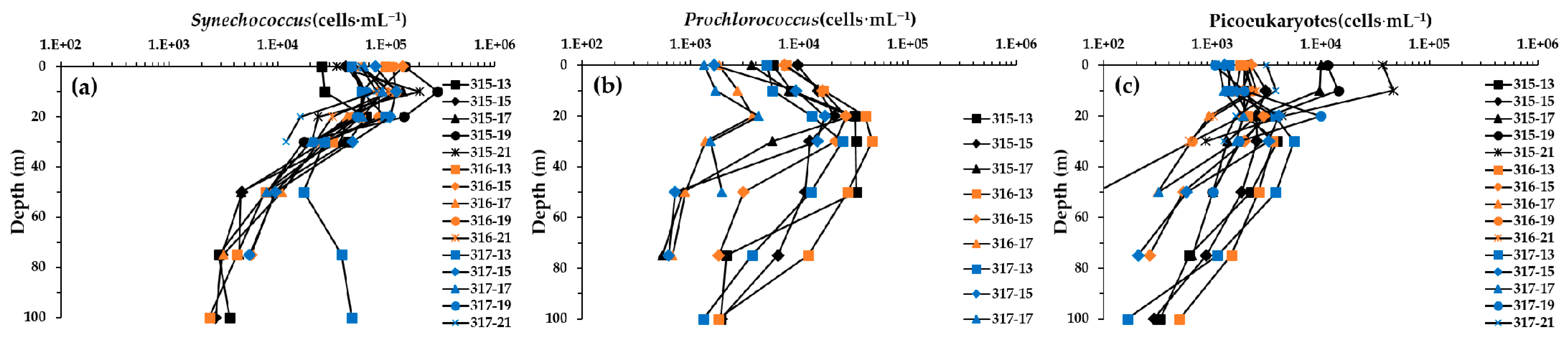
3.5. Picophytoplankton Cell Abundances

Figure 9 shows plots of the picophytoplankton standing stocks in three groups, as determined by flow cytometry. Synechococcus and Picoeukaryotes cells did not show spatially distinct distribution profiles, whereas Prochlorococcus cells appeared to be limited at some east-side sampling stations (13, 15, 17 on each line) and abundant in the west-side sampling stations. Regarding the vertical distribution of picophytoplankton in summer, all three genera showed the highest standing stocks at the depth where the thermocline formed (rather than at the surface layer) and gradually decreased below the thermocline.

4. Discussion

4.1. Changes in Phytoplankton-Community Structures in Response to Changes in the Summer Marine Environment

To determine the changes in the phytoplankton-community structure associated with changes in the marine environment of the northern East China Sea in the summer, we compared the data obtained from the same sampling stations (Lines 315 and 316) at the same depth in a previous study and in this study (Table 4). The comparison revealed decreased nutrients (especially phosphate) in the surface layer as a characteristic difference in the marine environment. In terms of the community structure, diatoms and dinoflagellates were identified as the dominant species in the previous study conducted by Oh [42], and nanoflagellates (≤20 μm) were identified as the dominant species in this study. This difference may be ascribed to decreased nutrients, especially in terms of phosphate. Among the nutrients flowing into the East China Sea, the DIN concentration in the estuary of the Changjiang River doubled from 1985 to 1998, and the DIN flux increased by 1.3-fold [43]. As a result, in the estuary and coastal waters of China, the area containing red tides increased from 2000 km2 in the 1980s to over 7000 km2 in the 2000s [44] and contributed to a 21-fold increase in the number of red tide occurrences. The frequent occurrence of red tides in the Changjiang River estuary consumes a large amount of phosphorus, resulting in a phosphorus deficiency (rather than excessive nitrogen) [11,45]. The Changjiang dilution water affects the northern East China Sea. However, the transport volume decreased by 9–18% after the construction of the Three Gorges Dam (2003–2009), and the amount of suspended solids decreased by up to 56% [46]. The decrease in the inflow of the Changjiang dilution water also decreased the amount of nutrients, which caused a change in the community structure of phytoplankton from being dominated by diatoms to being dominated by flagellates [47]. Furthermore, the main source of phosphorus in the East China Sea is the Kuroshio water mass, although its influence has recently decreased in the northern East China Sea. In this regard, it was reported that the phosphate inflow decreased as the influence of the Taiwan warm current (which is caused by upwelling of the Kuroshio water mass) also weakened [48]. The decrease in phosphate in the East China Sea caused a decrease in the proportion of diatoms from 85% in 1984 to 60% in 2000 [49]. These results were observed in both the East China Sea and the Yellow Sea. In this respect, Lin et al. [43] reported that the standing stock of diatoms markedly decreased from the 1980s to the 1990s because of the increased surface-water temperature of the Yellow Sea and decreased silicate and phosphate concentrations. Likewise, Lee [50] reported extremely low phosphate concentrations, even below the detection limit, in a study of the central part of the Yellow Sea in summer, which resulted in a phytoplankton transition due to phosphate restriction, in which flagellates (≤10 µm) were the dominant species at all sampling stations, except for some bottom layer-dominant species, such as species in the Navicula spp. and Skeleonema spp. It was also reported that the restriction of nutrients greatly affects the growth of phytoplankton when their concentrations fall below the minimum levels of DIN 1.0 μM, phosphate 0.2 μM, and silicate 2.0 μM [51]. Phosphate can also act as an important factor that hampers the growth of diatoms rather than flagellates [49], and if phosphate is deficient, then even if nitrate is abundant, phytoplankton cannot use nitrate, which hinders growth [52]. In this survey, the surface mixed layer, which accounted for 90% of the total standing stock, maintained sufficient nitrate and silicate concentrations, but had an extremely low phosphate concentration, even lower than 0.1 μM. The fact that nanoflagellates with relatively low nutrient requirements could dominate over diatoms in all sampling stations can be explained by the phosphate concentration acting as a limiting factor.

4.2. Changes in Phytoplankton Community Sizes and Structures in the Northern East China Sea

The results of this survey study indicated that the picophytoplankton contributed to >60% of the chl-a concentration in summer standing stock; in particular, the surface mixed layer (from the surface to a depth of 20 m), which had low nutrient concentrations, had the highest relative chl-a concentration. Spatially, higher chl-a percentages were observed at the east-side stations than at the west-side stations, where nutrient concentrations were relatively high (Table 3). These tendencies were verified using statistical analysis. RDA of environmental factors and the chl-a size revealed that the nutrient concentrations increased with increasing water depths, which was indicative of an environment where the nutrient availability became increasingly limited from the bottom layer to the surface layer due to strong stratification caused by the rise in the surface water temperature in summer. Regarding the relationship between the phytoplankton size and environmental factors, the fraction of nanophytoplankton increased toward the bottom layer, where nutrient concentrations were relatively high, whereas picophytoplankton were inversely related to all nutrients, showing the highest fraction at the surface layer, where nutrient concentrations were low. In particular, picophytoplankton had the strongest inverse correlation with phosphate, which was associated with extreme phosphate depletion in the surface mixed layer (Figure 10). Similar results have been reported in other sea areas in recent years. Size-fractionation analysis that integrated satellite-data analysis results and field observations in the Mediterranean Sea confirmed that picophytoplankton < 2 µm accounted for 31–92% of the total phytoplankton biomass with seasonal variations, primarily due to low nitrogen and phosphorus availability [53,54]. Agawin et al. [55] reported that the relative contribution of picophytoplankton to the total chl-a biomass was over 50% in Blanes Bay in the Mediterranean Sea, which was attributed primarily to high temperatures and nutrient-poor waters. The composition ratio of picophytoplankton was 44–90% and 54–64%, respectively, in the Mediterranean Tyrrhenian Sea and Levantine Basin waters [56,57]. An analysis of summer satellite data of the Yamato Basin and Japan Basin showed that the percentage of picophytoplankton was more than 50% [58]. In addition, the composition ratio of nanophytoplankton and picophytoplankton in many waters was reported to be over 60% [53,59,60,61,62] (Table 5). In summer surveys of the East Sea of Korea, the relative contribution of picophytoplankton to the total chl-a biomass ranged from 35 to 63% [58,63], whereas those of nanophytoplankton and picophytoplankton (≤20 µm) were 74% on average in the surface layer of the eastern Yellow Sea, in a study focused on the dominance of small phytoplankton [50]. Similarly, Furuya et al. [64] showed that picophytoplankton made a high relative contribution (up to 80%) due to the oligotrophic environment of the surface layer in a summer survey of the northern East China Sea. Son et al. [33] also reported that their analysis of long-term satellite observations of the chl-a biomass led to the finding that the contribution of microphytoplankton to the chl-a concentration sharply decreased in the northern East China Sea, whereas those of nanophytoplankton and picophytoplankton increased. These results have a common denominator in that they were derived from oligotrophic environments, where smaller phytoplankton cells had larger surface areas per unit volume, making small phytoplankton become dominant, owing to their capacity for rapid nutrient exchange through the cell surface [65,66,67].
Miniaturization of the phytoplankton size can result in decreased primary productivity. Indeed, analysis of primary productivity data derived from the Moderate Resolution Imaging Spectroradiometer Aqua led to a report showing that the annual primary production in the East Sea is decreasing by 13% per decade, as a result of an increase in the relative contribution of picophytoplankton (≤2 µm) to the total biomass [68]. Moreover, Lee et al. [63] verified a strong inverse correlation between the dominance rate of phytoplankton of ≤5 µm and the total primary production in the Amundsen Sea and attributed this to the low rate of carbon uptake by small phytoplankton. The miniaturization of phytoplankton also affects the food web, and it is projected that the increase in picophytoplankton abundance would lead to the dominance of microzooplankton (<200 µm) and gelatinous zooplankton (salps, doliolids, and ctenophores) and a decrease in biomass [69]. Moreover, a previous study showed that mesozooplankton (<200 µm), e.g., copepods, did not directly feed on picophytoplankton, but rather indirectly fed on ciliates that feed on picophytoplankton [70]. Accordingly, as the dominance of picophytoplankton increases, the biomass of mesozooplankton that do not directly feed on them will likely decrease. Consequently, the marine food chain will likely change from a simple diatom-based web with high primary productivity to a complex microbial food web centering on small phytoplankton with low productivity, negatively affecting overall marine productivity and reducing the efficiency of carbon transfer to consumers at higher trophic levels (Figure 11).

Author Contributions

Conceptualization, K.-W.P. and S.-H.Y.; methodology K.-W.P. and M.-H.Y.; validation, K.-W.P. and S.-H.Y.; formal analysis, K.-W.P., S.-Y.M. and M.-H.Y.; investigation, K.-W.P., H.-J.O., S.-Y.M., M.-H.Y. and S.-H.Y.; data curation, K.-W.P.; writing—original draft preparation, K.-W.P.; writing—review and editing, S.-H.Y.; visualization, K.-W.P.; supervision, S.-H.Y.; project administration, H.-J.O. and S.-H.Y.; funding acquisition, H.-J.O. and S.-H.Y. All authors have read and agreed to the published version of the manuscript.

Funding

This research was supported by the “Development of assessment technology on the structure variations in marine ecosystem (R2022073)” funded by the National Institute of Fisheries Science (NIFS), Korea.

Data Availability Statement

Not applicable.

Acknowledgments

We appreciate the captains and crew of R/V Tamgu 3 for their assistance with collecting our samples. We would also like to thank the researchers for their assistance with sample analysis.

Conflicts of Interest

The authors declare no conflict of interest.

References

  1. Zhang, Q.L.; Weng, X.C. Analysis of water masses in the south Yellow Sea in spring. Oceanol. Limnol. Sin. 1996, 27, 421–428. [Google Scholar]
  2. Rho, H.K. Studies on Marine Environment of Fishing Grounds in the Waters around Cheju Island. Ph.D. Thesis, Tokyo University, Tokyo, Japan, 1985. [Google Scholar]
  3. Miyaji, K. Studies on the eddies associated with the meander of the Kuroshio in the waters off southwest coast of Kyushu and their effects on egg and larval transport. Bull. Seikai Nat. Fish. Res. Inst. 1991, 69, 1–77. [Google Scholar]
  4. Guo, Y.J.; Zhang, Y.S. Characteristics of phytoplankton distribution in Yellow Sea. J. Yellow Sea 1996, 2, 90–103. [Google Scholar]
  5. Simpson, J.H.; Pingree, R.D. Shallow sea fronts produced by tidal stirring. In Oceanic Fronts in Coastal Processes; Bowman, M.J., Esaias, W.E., Eds.; Springer: Berlin/Heidelberg, Germany, 1978; pp. 29–47. [Google Scholar]
  6. Beardsley, R.; Limebumer, R.; Yu, H.; Cannon, G.A. Discharge of the Changjiang (Yangtze River) into the East China Sea. Cont. Shelf Res. 1985, 4, 57–76. [Google Scholar] [CrossRef]
  7. Su, Y.S.; Weng, X.C. Water masses in China Seas. In Oceanography of China Seas; Zhou, D., Liang, Y.B., Zeng, C.K., Eds.; Springer: Dordrecht, The Netherlands, 1994; pp. 3–16. [Google Scholar]
  8. Edmond, J.M.; Spivack, A.; Grant, B.C.; Chen, Z.; Chen, S.; Zeng, X. Chemical dynamics of the Changjiang Estuary. Cont. Shelf Res. 1985, 4, 17–36. [Google Scholar] [CrossRef]
  9. Hama, T.; Shin, K.H.; Handa, N. Spatial variability in the primary productivity in the East China Sea and its adjacent water. J. Oceanogr. 1997, 53, 41–51. [Google Scholar] [CrossRef]
  10. Gong, G.C.; Wen, Y.H.; Wang, B.W.; Liu, G.J. Seasonal variation of chlorophyll a concentration, primary production and environmental conditions in the subtropical East China Sea. Deep Sea Res. Part II 2003, 50, 1219–1236. [Google Scholar] [CrossRef]
  11. Chen, Y.L.; Chen, H.Y.; Gong, G.C.; Lin, Y.H.; Jan, S.; Takahashi, M. Phytoplankton production during a summer coastal upwelling in the East China Sea. Cont. Shelf Res. 2004, 24, 1321–1338. [Google Scholar] [CrossRef]
  12. Koroji, K.; Matsusaki, M. Present activity on marine biology in Japan Meteorological Agency. Sokuko Jiho 1980, 47, 19–21. [Google Scholar]
  13. Chin, T.G.; Cheng, Z.M.; Lin, J.; Lin, S. Diatoms from the surface sediments of the east China Sea. Acta Oceanol. Sin. 1980, 2, 97–110. [Google Scholar]
  14. Huang, R. The influence of hydrography on the distribution of phytoplankton in the southern Taiwan strait. Estuar. Coast. Shelf Sci. 1988, 26, 643–656. [Google Scholar] [CrossRef]
  15. Koizumi, I. Pliocene and Pleistocene diatom datum levels related with Paleoceanography in the northwest Pacific. Mar. Micropaleontol. 1986, 10, 309–325. [Google Scholar] [CrossRef]
  16. Yu, J.L.; Li, R.X. Species composition and quantitative distribution of planktonic diatom in the Kuroshio current and its adjacent waters. In Selected Papers on the Investigation of Kuroshio; Su, J.L., Ed.; Ocean Press: Beijing, China, 1990; Volume 2, pp. 57–66. [Google Scholar]
  17. Guo, Y.J. The Kuroshio, part 2. Primary productivity and phytoplankton. Oceanogr. Mar. 1991, 29, 155–189. [Google Scholar]
  18. Huang, R. Phytoplankton distribution in the South China Sea and Kuroshio-flowing region of Taiwan. Acta Oceanogr. Taiwan. 1993, 31, 73–82. [Google Scholar]
  19. Matsuda, O.; Nishi, Y.; Yoon, Y.H.; Endo, T. Observation of thermohaline structure and phytoplankton biomass the shelf front of East China Sea during early summer. J. Fac. Appl. Biol. Sci. 1989, 28, 27–35. [Google Scholar]
  20. Kamiya, H. The correlation between appearance of phytoplankton and the sea condition. Umi Sora 1991, 67, 153–162. [Google Scholar]
  21. Ueno, S. Phytoplankton communities and their relation to the water types in the vicinity of the Kuroshio front in the East China. Sea J. Shimonoseki Univ. Fish. 1993, 41, 251–256. [Google Scholar]
  22. Meng, F.; Huang, F.; Zhaodang, M.; Qinliang, L. On the composition and distribution of zooplankton species in the Kuroshio region in the north of the East China Sea. In Selected Papers on the Investigation of Kuroshio; Su, J.L., Ed.; Ocean Press: Beijing, China, 1991; Volume 3, pp. 150–161. [Google Scholar]
  23. Zhang, H.Q. Relationship between zooplankton distribution and hydrographic characteristics of the southern Yellow Sea. Yellow Sea 1995, 1, 50–67. [Google Scholar]
  24. Choi, C.H.; Lee, C.R.; Kang, H.K.; Kang, K.A. Characteristics and variation of size-fractionated zooplankton biomass in the northern East China Sea. Ocean Polar Res. 2011, 33, 135–147. [Google Scholar] [CrossRef] [Green Version]
  25. Oh, G.S. Characteristics and Variation of Zooplankton Community Structure in the Northern East China Sea. Master’s Thesis, Chonnam National University, Yeosu, Korea, 2012. [Google Scholar]
  26. Dong, H.; Ren, D.; Li, B. The distribution and influential factors of oxygen and phosphate in Kuroshio area of the East China Sea north to 30 degree N in summer and winter 1987. In Selected Papers on the Investigation of Kuroshio; Su, J.L., Ed.; Ocean Press: Beijing, China, 1990; Volume 2, pp. 208–217. [Google Scholar]
  27. Noh, J.H. A Study on the Phytoplankton Distribution in the Yellow Sea and the East China Sea. Master’s Thesis, Inha University, Incheon, Korea, 1995. [Google Scholar]
  28. Yoon, Y.H.; Park, J.S.; Soh, H.Y.; Hwang, D.J. Spatial distribution of phytoplankton community and red tide of Dinoflagellate, Prorocentrum donghaiense in the East China Sea during early summer. Korean J. Environ. Biol. 2003, 21, 132–141. [Google Scholar]
  29. Yoon, Y.H.; Park, J.S.; Park, Y.G.; Soh, H.Y.; Hwang, D.J. A characteristics of thermohaline structure and phytoplankton community from southwestern parts of the East China Sea during early summer, 2004. Bull. Korean Soc. Fish. 2005, 41, 129–139. [Google Scholar]
  30. Noh, J.H.; Yoo, S.J.; Lee, J.A.; Kim, H.C.; Lee, J.H. Phytoplankton in the waters of the Ieodo Ocean Research Station determined by microscopy, flow cytometry, HPLC pigment data and remote sensing. Ocean Polar Res. 2005, 27, 397–417. [Google Scholar]
  31. Kim, D.S.; Shim, J.H.; Lee, J.A.; Kang, Y.C. The distribution of nutrients and chlorophyll in the northern East China Sea during the spring and summer. Ocean Polar Res. 2005, 27, 251–263. [Google Scholar] [CrossRef]
  32. Kim, D.S.; Kim, K.H.; Shim, J.H.; Yoo, S.J. The distribution and interannual variation in nutrients, chlorophyll-a, and suspended solids in the northern East China Sea during the summer. Ocean Polar Res. 2007, 29, 193–204. [Google Scholar] [CrossRef] [Green Version]
  33. Son, Y.B.; Ryu, J.H.; Noh, J.H.; Ju, S.J.; Kim, S.H. Climatological variability of satellite-derived sea surface temperature and chlorophyll in the south sea of Korea and East China Sea. Ocean Polar Res. 2012, 34, 201–218. [Google Scholar] [CrossRef] [Green Version]
  34. Gong, G.C.; Chang, J.; Chiang, K.P.; Hsiung, T.M.; Hung, C.C.; Duan, S.W.; Codispti, L.A. Reduction of primary production and changing of nutrient ratio in the East China Sea: Effect of the Three Gorges Dam? Geophys. Res. Lett. 2006, 33. [Google Scholar] [CrossRef] [Green Version]
  35. Jiaoa, N.; Zhang, Y.; Zeng, Y.; Gardner, W.D.; Mishonov, A.V.; Richardson, M.J.; Hong, N.; Pan, D.; Yan, X.H.; Jo, Y.H.; et al. Ecological anomalies in the East China Sea: Impacts of the Three Gorges Dam? Water Res. 2007, 41, 1287–1293. [Google Scholar] [CrossRef]
  36. Smayda, T.J. Biogeographical meaning indicators. In Phytoplankton Manual; Sournia, A., Ed.; United Nations Educational, Scientific, and Cultural Organization: Paris, France, 1978; pp. 225–229. [Google Scholar]
  37. Rines, J.E.B.; Hargraves, P.E. The Chaetoceros Ehrenberg (Bacillariophyceae) Flora of Narragansett Bay; Schweizebart Science: Stuttgart, Germany, 1988. [Google Scholar]
  38. Round, F.E.; Crawfor, R.M.; Mann, D.G. The Diatoms; Cambridge: New York, NY, USA, 1990. [Google Scholar]
  39. Shim, J.H. Flora and fauna of Korea. In Marine Phytoplankton; Ministry of Education: Seoul, Korea, 1994; Volume 34. [Google Scholar]
  40. Tomas, C.R. Identifying Marine Phytoplankton; Academic Press: Cambridge, MA, USA, 1997. [Google Scholar]
  41. Parsons, T.R.; Maita, Y.; Lalli, C.M. A Manual of Biological and Chemical Methods for Seawater Analysis; Pergamon Press: Oxford, UK, 1984. [Google Scholar]
  42. Oh, H.J. Ecological Characteristics of Phytoplankton in the Northern Part of East China Sea. Ph.D. Thesis, Pusan National University, Busan, Korea, 1998. [Google Scholar]
  43. Lin, C.; Ning, X.; Su, J.; Lin, Y.; Xu, B. Environmental changes and the responses of the ecosystems of the Yellow Sea during 1976–2000. J. Mar. Syst. 2005, 55, 223–234. [Google Scholar] [CrossRef]
  44. Li, M.K.; Xu, K.; Watanabe, M.; Chen, Z. Long-term variations in dissolved silicate, nitrogen, and phosphorus flux from the Changjiang River into the East China Sea and impacts on estuarine ecosystem. Estuar. Coast. Shelf Sci. 2007, 71, 3–12. [Google Scholar] [CrossRef]
  45. Li, H.M.; Tang, H.J.; Shi, X.Y.; Zhang, C.S.; Wang, X.L. Increased nutrient loads from the Changjiang (Yangtze) River have led to increased Harmful Algal Blooms. Harmful Algae 2014, 39, 92–101. [Google Scholar] [CrossRef]
  46. Ministry of Land, Transport and Maritime Affairs. The Study of Oceanographic Environmental Impact in the South Sea (East China Sea) due to the Three Gorges Dam; Ministry of Land, Transport and Maritime Affairs: Seoul, Korea, 2009; pp. 7–175.
  47. Jiang, Z.; Liu, J.; Chen, J.; Chen, Q.; Yan, X.; Xuan, J.; Zeng, J. Responses of summer phytoplankton community to drastic environmental changes in the 664 Changjiang (Yangtze River) estuary during the past 50 years. Water Res. 2014, 54, 1–11. [Google Scholar] [CrossRef]
  48. Youn, S.C.; Suk, H.Y.; Whang, J.D.; Suh, Y.S.; Yoon, Y.Y. Long-term variation in ocean environmental conditions of the northern East China Sea. J. Korean Soc. Mar. Environ. Energy 2015, 18, 189–206. [Google Scholar] [CrossRef]
  49. Zhou, M.J.; Shen, Z.L.; Yu, R.C. Responses of a coastal phytoplankton community to increased nutrient input from the Changjiang (Yangtze) River. Cont. Shelf Res. 2008, 28, 1483–1489. [Google Scholar] [CrossRef]
  50. Lee, Y.J. Phytoplankton Dynamics and Primary Production in the Yellow Sea during Winter and Summer. Ph.D. Thesis, Inha University, Incheon, Korea, 2012. [Google Scholar]
  51. Dortch, Q.; Whitledge, T.E. Does nitrogen or silicon limit phytoplankton production in the Mississippi River plume and nearby regions? Cont. Shelf Res. 1992, 12, 1293–1309. [Google Scholar] [CrossRef]
  52. Chen, Y.L.; Lu, H.; Shiah, F.; Gong, G.; Liu, K.; Kanda, J. New production and f-ratio on the continental shelf of the East China Sea: Comparisons between nitrate inputs from the subsurface Kuroshio Current and the Changjiang River. Estuar. Coast. Shelf Sci. 1999, 48, 59–75. [Google Scholar] [CrossRef]
  53. Magazzu, G.; Decembrini, F. Primary production, biomass and abundance of phototrophic picoplankton in the Mediterranean Sea: A review. Aquat. Microb. Ecol. 1995, 9, 97–104. [Google Scholar] [CrossRef] [Green Version]
  54. Uitz, J.; Stramski, D.; Gentili, B.; D’Ortenzio, F.; Claustre, H. Estimates of phytoplankton class-specific and total primary production in the Mediterranean Sea from satellite ocean color observations. Glob. Biogeochem. Cycles 2012, 26. [Google Scholar] [CrossRef]
  55. Agawin, N.S.R.; Duarte, C.M.; Agusti, S. Nutrient and temperature control of the contribution of picoplankton to phytoplankton biomass and production. Limnol. Oceanogr. 2000, 45, 591–600. [Google Scholar] [CrossRef]
  56. Zohary, T.; Brenner, S.; Krom, M.D.; Angel, D.L.; Kress, N.; Li, W.K.W.; Neori, A.; Yacobi, Y.Z. Buildup of microbial biomass during deep winter mixing in a Mediterranean warm-core eddy. Mar. Ecol. Prog. Ser. 1998, 167, 47–57. [Google Scholar] [CrossRef]
  57. Decembrini, F.; Caroppo, C.; Azzaro, M. Size structure and production of phytoplankton community and carbon pathways channeling in the southern Tyrrhenian Sea (western Mediterranean). Deep Sea Res. Part II 2009, 56, 687–699. [Google Scholar] [CrossRef]
  58. Kwak, J.H.; Lee, S.H.; Hwan, J.; Suh, Y.-S.; Park, H.J.; Chang, K.-I.; Kim, K.-R.; Kang, C.K. Summer primary productivity and phytoplankton community composition driven by different hydrographic structures in the East/Japan Sea and the Western Subarctic Pacific. J. Geophys. Res. Oceans 2014, 119, 4505–4519. [Google Scholar] [CrossRef]
  59. Revelante, N.; Gilmartin, M. The relative increase of larger phytoplankton in a subsurface chlorophyll maximum of the northern Adriatic Sea. J. Plankton Res. 1995, 17, 1535–1562. [Google Scholar] [CrossRef]
  60. Marañón, E.; Holligan, P.M.; Barciela, R.; González, N.; Mouriño, B.; Pazó, M.J.; Varela, M. Patterns of phytoplankton size structure and productivity in contrasting open-ocean environments. Mar. Ecol. Prog. Ser. 2001, 216, 43–56. [Google Scholar] [CrossRef] [Green Version]
  61. Morán, X.A.G.; Taupier-Letage, I.; Vázquez-Domínguez, E.; Ruiz, S.; Arin, L.; Raimbault, P.; Estrada, M. Physical-biological coupling in the Algerian Basin (SW Mediterranean): Influence of mesoscale instabilities on the biomass and production of phytoplankton and bacterioplankton. Deep Sea Res. Part I 2001, 48, 405–437. [Google Scholar] [CrossRef]
  62. Ning, X.; Chai, F.; Xue, H.; Cai, Y.; Liu, C.; Shi, J. Physical-biological oceanographic coupling influencing phytoplankton and primary production in the South China Sea. J. Geophys. Res. 2005, 109, C10005. [Google Scholar] [CrossRef] [Green Version]
  63. Lee, S.H.; Joo, H.T.; Lee, J.H.; Lee, J.H.; Kang, J.J.; Lee, H.W.; Lee, D.B.; Kang, C.K. Carbon uptake rates of phytoplankton in the Northern East/Japan Sea. Deep Sea Res. Part II 2017, 143, 45–53. [Google Scholar] [CrossRef]
  64. Furuya, K.; Hayashi, M.; Yabushita, Y.; Ishikawa, A. Phytoplankton dynamics in the East China Sea in spring and summer as revealed by HPLC derived pigment signatures. Deep Sea Res. Part II 2003, 50, 367–387. [Google Scholar] [CrossRef]
  65. Raven, J.R. The twelfth tansley lecture. Small is beautiful: The picophytoplankton. Funct. Ecol. 1998, 12, 503–513. [Google Scholar] [CrossRef]
  66. Litchman, E.; Klausmeier, C.A.; Schofield, O.M.; Falkowski, P.G. The role of functional traits and trade-offs in structuring phytoplankton communities: Scaling from cellular to ecosystem level. Ecol. Lett. 2007, 10, 1170–1181. [Google Scholar] [CrossRef]
  67. Longhurst, A.R. Ecological Geography of the Sea; Academic Press: London, UK, 2010. [Google Scholar]
  68. Joo, H.T.; Son, S.H.; Park, J.W.; Kang, J.J.; Jeong, J.Y.; Lee, C.I.; Kang, C.K.; Lee, S.H. Long-term pattern of primary productivity in the East/Japan Sea based on ocean color data derived from MODIS-aqua. Remote Sens. 2016, 8, 25. [Google Scholar] [CrossRef] [Green Version]
  69. Richardson, A.J. In hot water: Zooplankton and climate change. ICES J. Mar. Sci. 2008, 65, 279–295. [Google Scholar] [CrossRef] [Green Version]
  70. Lee, C.R.; Kang, H.K.; Choi, K.H. Latitudinal distribution of mesozooplankton community in the northwestern Pacific Ocean. Ocean Polar Res. 2011, 33, 337–347. [Google Scholar] [CrossRef] [Green Version]
Figure 1. Sampling station in the northern East China Sea, 2016–2020. CDW: Changjiang diluted water; YSWC: Yellow Sea cold water; KW: Kuroshio water; TCWW: Taiwan current warm water; TSW: Tsushima surface water.
Jmse 10 00315 g001
Figure 2. Flow-cytometric analysis of a picophytoplankton sample. The signatures of each picoplankton group were discriminated based on their orange and red fluorescence intensities. PerCP-H: red-fluorescence, PE-H: orange-fluorescence, P1: picoeukaryote count, P2: Synechococcus count, P6: Prochlorococcus count.
Jmse 10 00315 g002
Figure 3. Spatial distribution of the average surface temperature (a, °C) and average surface salinity (b, psu) in the northern East China Sea from 2016 to 2020.
Jmse 10 00315 g003
Figure 4. Vertical distribution of average surface temperatures (a, °C) and average surface salinities (b, psu) in the northern East China Sea from 2016 to 2020.
Jmse 10 00315 g004
Figure 5. Spatial distributions of average surface dissolved inorganic nitrogen (a, DIN), PO4 (b), and SiO2 (c) concentrations (in μM) in the northern East China Sea from 2016 to 2020.
Jmse 10 00315 g005
Figure 6. Vertical distribution of the average DIN (a), PO4 (b), and SiO2 (c) concentrations (in μM) in the northern East China Sea from 2016 to 2020.
Jmse 10 00315 g006
Figure 7. Spatial distributions of the average surface chl-a concentrations (µg·L−1) in the northern East China Sea from 2016 to 2020.
Jmse 10 00315 g007
Figure 8. Vertical distributions of the average chl-a concentrations (µg·L−1) in the northern East China Sea from 2016 to 2020.
Jmse 10 00315 g008
Figure 9. Vertical distributions of Synechococcus (a), Prochlorococcus (b), and picoeukaryote (c) cell abundances (cells·mL1) found at each station in the northern East China Sea from 2016 to 2020.
Jmse 10 00315 g009
Figure 10. Redundancy analysis (RDA) ordination plots showing relationships between environmental and biological conditions in the northern East China Sea.
Jmse 10 00315 g010
Figure 11. Changes in the food chain due to succession of the phytoplankton community in the northern East China Sea.
Jmse 10 00315 g011
Table 1. Description of the sampling sites in the northern East China Sea for the cruise period from 2016 to 2020.
StationLatitudeLongitudeBottom Depth (m)
315-1332.5127.0125
315-1532.5126.5107
315-1732.5125.991
315-1932.5125.368
315-2132.5124.546
316-1332.0127.0119
316-1532.0126.599
316-1732.0125.976
316-1932.0125.355
316-2132.0124.539
317-1331.5127.0105
317-1531.5126.588
317-1731.5125.967
317-1931.5125.354
317-2131.5124.546
Table 2. Dominant phytoplankton taxa in the northern East China Sea from 2016 to 2020.
Dominance20162017201820192020
1stNanoflagellates (<20 µm; 50.5%)Nanoflagellates
(<20 µm; 50.1%)
Nanoflagellates (<20 µm; 43.1%)Nanoflagellates (<20 µm; 68.6%)Nanoflagellates (<20 µm; 69.7%)
2ndScrippsiella acuminata (15.2%)Chaetoceros lorenzianus (14.3%)Paralia sulcata (10.2%)Alexandrium spp. (8.4%)Paralia sulcata (6.5%)
3rdGuinardia flaccida (9.4%)Diploneis spp. (11.0%)Chaetoceros spp. (6.0%)
Table 3. Vertical variation of the chl-a size composition in the northern East China Sea from 2016 to 2020.
315 LineChl-a Size Composition (%)316 LineChl-a Size Composition (%)317 LineChl-a Size Composition (%)
St.*Depth (m)MNPSt.Depth (m)MNPSt.Depth (m)MNP
13012.018.469.613012.614.073.413020.215.064.8
1010.717.471.9109.313.777.01016.817.066.2
205.218.676.22017.016.166.92016.618.964.5
3010.521.268.33010.628.860.63012.617.070.4
5013.221.964.95011.319.868.95017.825.356.9
7518.431.550.17513.727.658.77518.630.351.1
10018.244.537.310016.742.041.310023.942.333.8
15014.332.653.115017.922.359.815012.422.964.7
108.623.967.51011.921.067.11024.317.358.4
2014.218.567.3202.922.274.92020.521.757.8
3025.821.053.23015.029.555.53023.227.549.3
5012.122.665.35019.947.232.95013.541.744.8
7510.033.956.17513.058.228.87523.150.926.0
10012.752.534.810017.758.923.4
17017.520.062.517040.818.540.717030.614.554.9
1019.821.159.11032.517.350.21026.018.355.7
2010.029.660.42024.120.9552040.716.742.6
3013.735.850.53027.330.941.83040.722.337.0
509.947.842.35024.851.224.05024.345.630.1
7526.952.820.37523.759.916.4
19023.819.456.819037.223.139.719030.921.247.9
1020.721.457.91034.721.244.11027.318.354.4
2023.427.549.12027.128.344.62028.819.951.3
308.940.650.53037.140.322.63044.230.525.3
5020.858.520.75025.655.718.75019.647.033.4
21029.915.854.321053.618.128.321034.429.636.0
1041.919.738.41045.817.736.51030.631.937.5
2040.432.327.32047.123.129.82054.116.829.1
3051.429.619.03035.534.530.03042.825.032.2
Mean18.829.351.9 Mean24.430.445.2 Mean26.626.147.3
SD10.912.116.0 SD12.914.718.3 SD10.610.713.7
*St.: station; M: micro (>20 µm); N: nano (20 µm ≥ chl-a > 3 µm); P: pico (≤3 µm).
Table 4. Comparison of environmental variables and dominant species in the northern East China Sea between August 1998 [42] and August 2016 to 2020 (this study).
Parameters August 1998August 2016–2020
Temperature (°C)Surface27.4–29.4 (28.7 ± 0.5)25.4–31.3 (28.0 ± 1.4)
Vertical12.7–29.4 (21.5 ± 5.9)11.8–31.3 (23.1 ± 5.5)
SalinitySurface26.7–29.7 (28.3 ± 0.9)26.2–34.0 (30.1 ± 1.9)
Vertical27.5–34.7 (31.2 ± 2.5)26.2–34.6 (31.7 ± 1.9)
Nitrite (µM)Surface0.07–0.36 (0.21 ± 0.08)0.01–0.16 (0.05 ± 0.04)
Vertical0.07–0.57 (0.19 ± 0.14)0.01–1.61 (0.15 ± 0.26)
Nitrate (µM)Surface1.26–3.54 (2.51 ± 0.66)0.12–11.37 (2.77 ± 2.70)
Vertical0.87–3.54 (2.05 ± 0.74)0.09–35.40 (5.87 ± 5.54)
Phosphate (µM)Surface0.16–0.45 (0.25 ± 0.09)ND–0.16 (0.05 ± 0.04)
Vertical0.16–1.03 (0.39 ± 0.23)ND–0.82 (0.21 ± 0.24)
Silicate (µM)Surface8.95–13.77 (9.69 ± 1.45)0.01–11.46 (4.23 ± 3.10)
Vertical8.95–13.77 (9.59 ± 0.88)0.01–40.17 (7.87 ± 5.71)
Dominant species Pseudonitzschia pungens
Prorocentrum dentatum
Skeleonema costatum
Nanoflagellates (<20 µm)
Scrippsiella acuminata
Paralia sulcata
Values in parentheses are means.
Table 5. Size fractionation of phytoplankton observed in the different coastal waters of the northern East China Sea and global waters.
Relative Ratio (%)
AreaDatePico SizeNano SizeMicro SizeReferences
Northen East China Sea2018–2020/
seasonally
45.631.223.2This study
Blanes Bay1997/summer>50 [55]
Levantine BasinMarch 199254.3–64.2 [56]
Tyrrhenian Sea (South)July 200544–81 [57]
December 200576–90
Western Subarctic Pacific23–29 June 201063 [58]
Japan Basin5–11 July 201056
Yamato Basin18–20 July 201056
Ulleung Basin22–24 July 201038
Mediterranean Sea 31–92 [53]
Adriatic Sea (North)August 1986 and 1988; July 1987 10–23[59]
Atlantic Meridional Transect
(Oligortophic)
April, October 1996
April, October 1997
80164[60]
Algerian BasinOctober 199642–6238–58 [61]
South China Seasummer 1998632216[62]
winter 1998511436
Publisher’s Note: MDPI stays neutral with regard to jurisdictional claims in published maps and institutional affiliations.

