Optimization of the Wake Oscillator for Transversal VIV

 , and
, and
Abstract
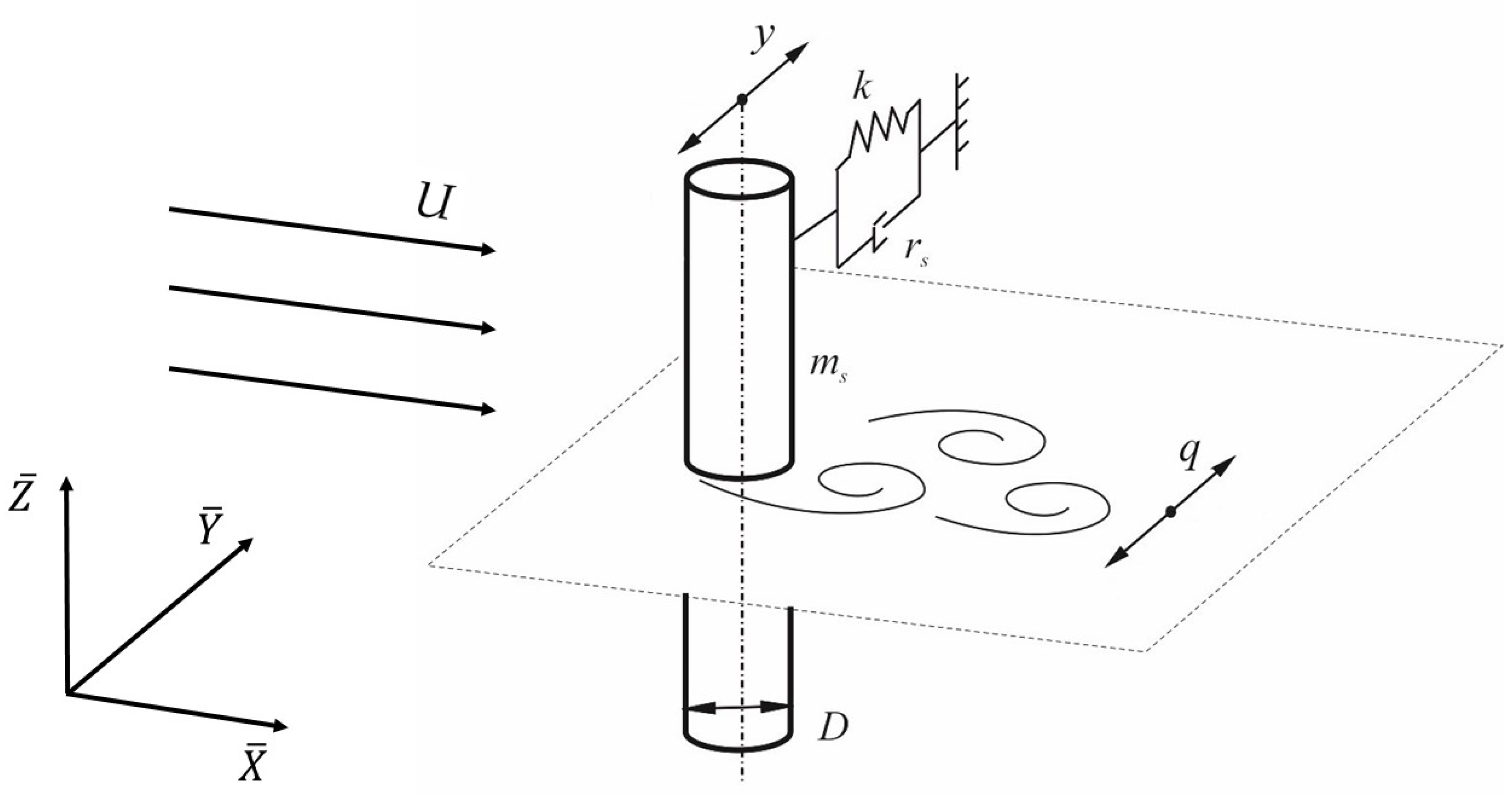
:1. Introduction
2. Optimization of Mathematical Model
3. Optimization of Empirical Coefficients
4. Results and Discussion
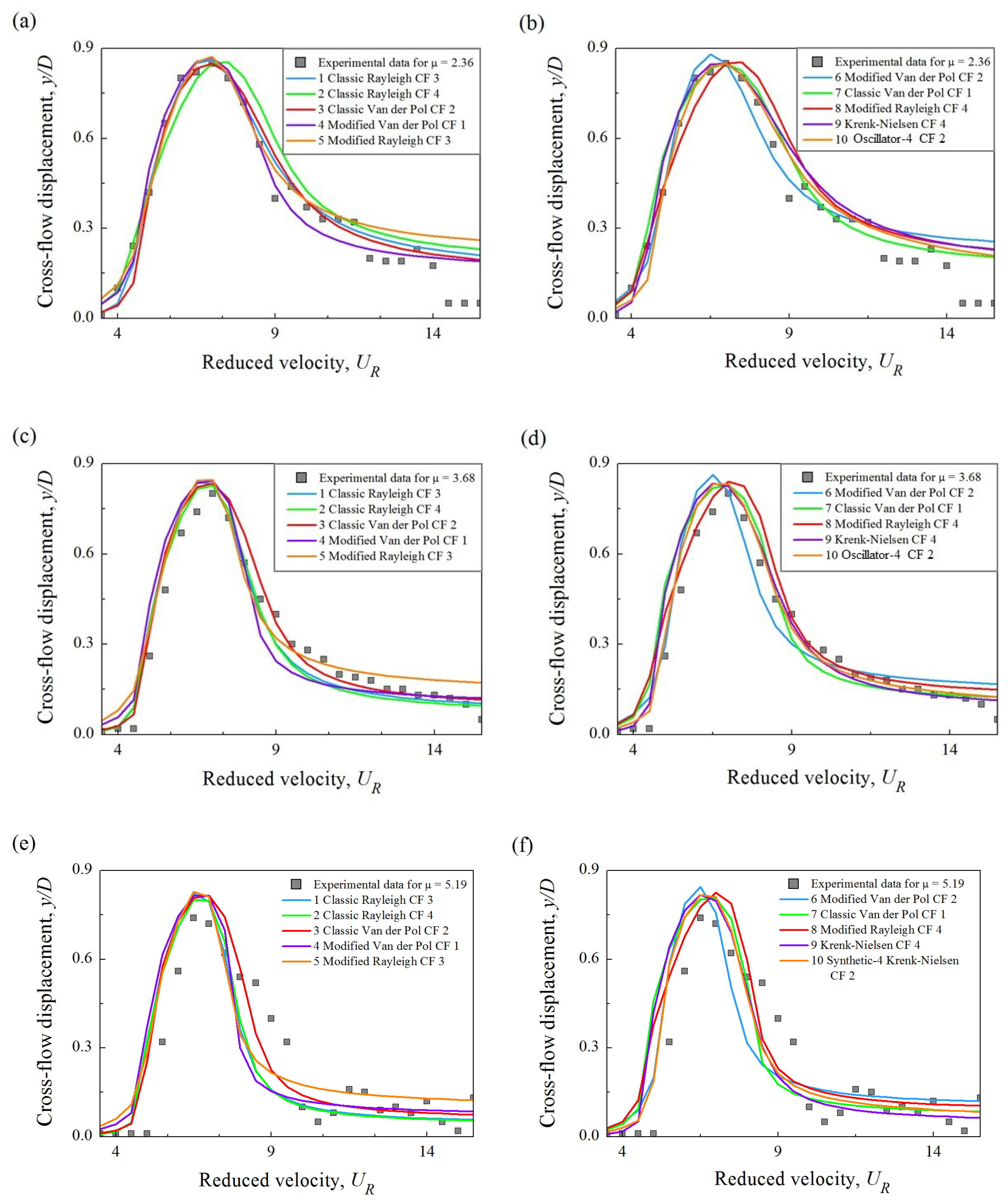
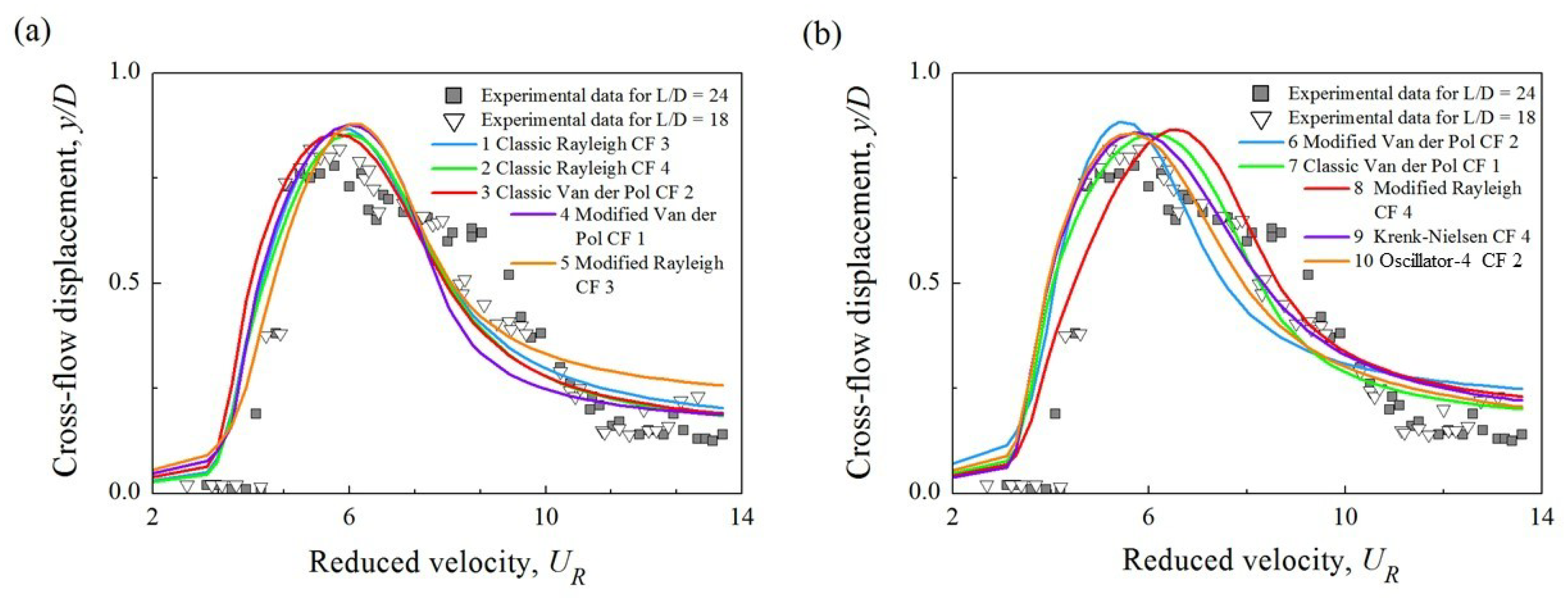
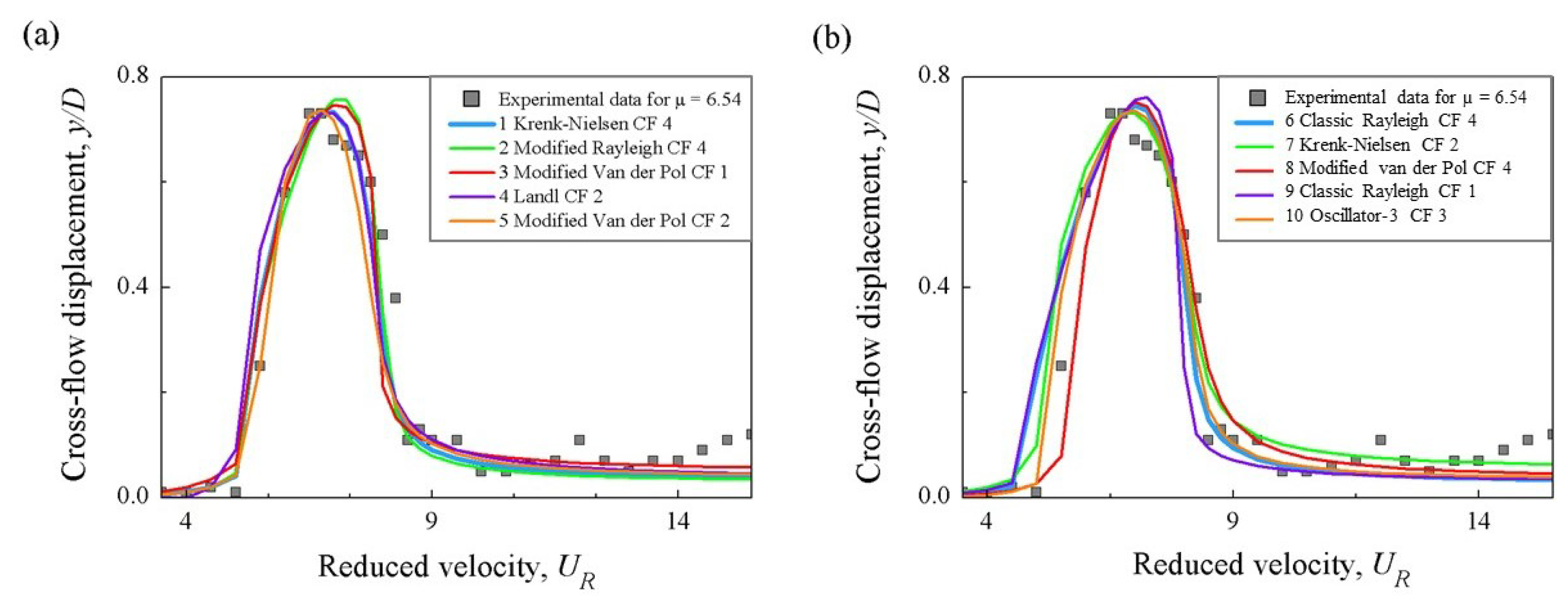
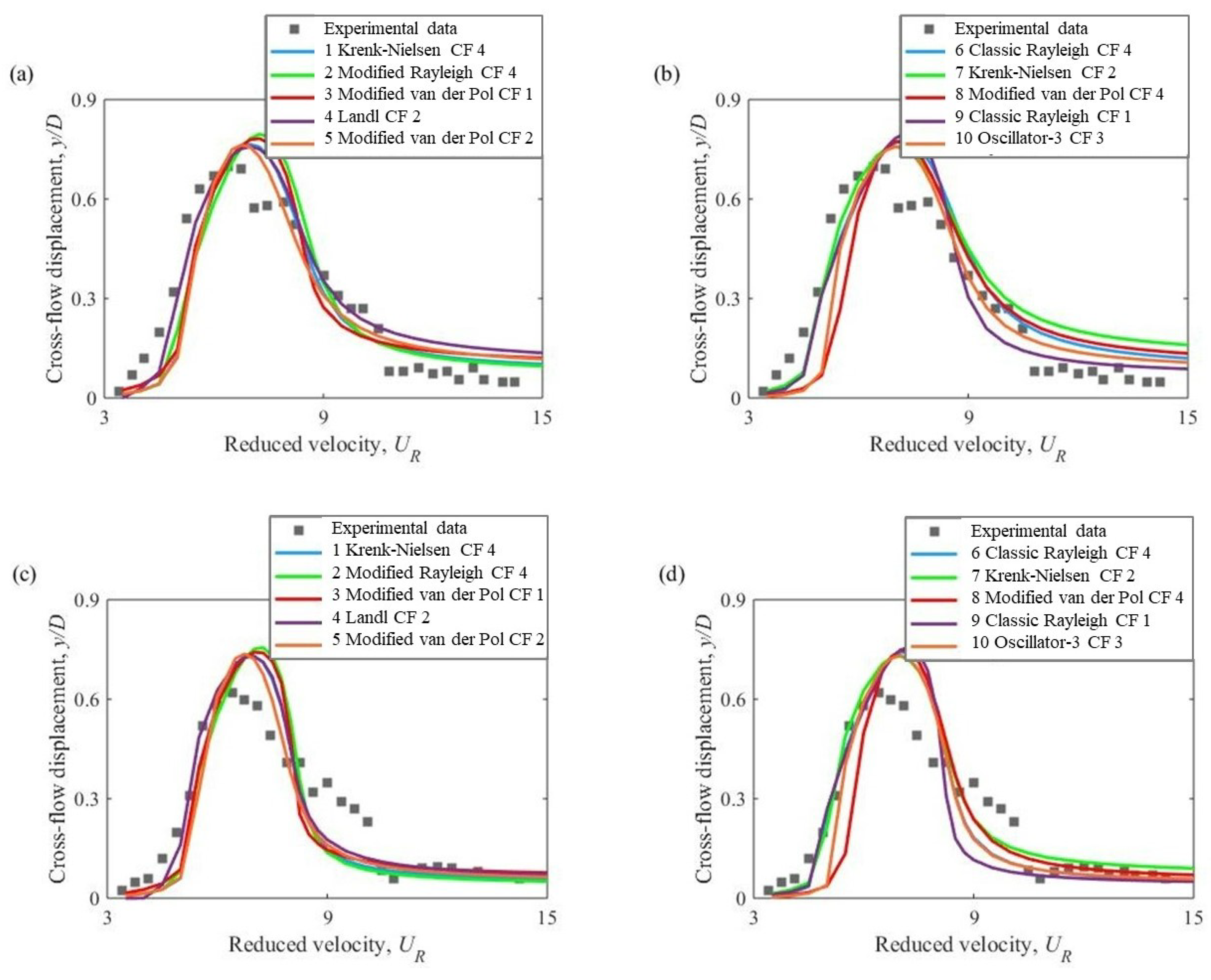
4.1. Models Calibrated with Low Mass Ratio
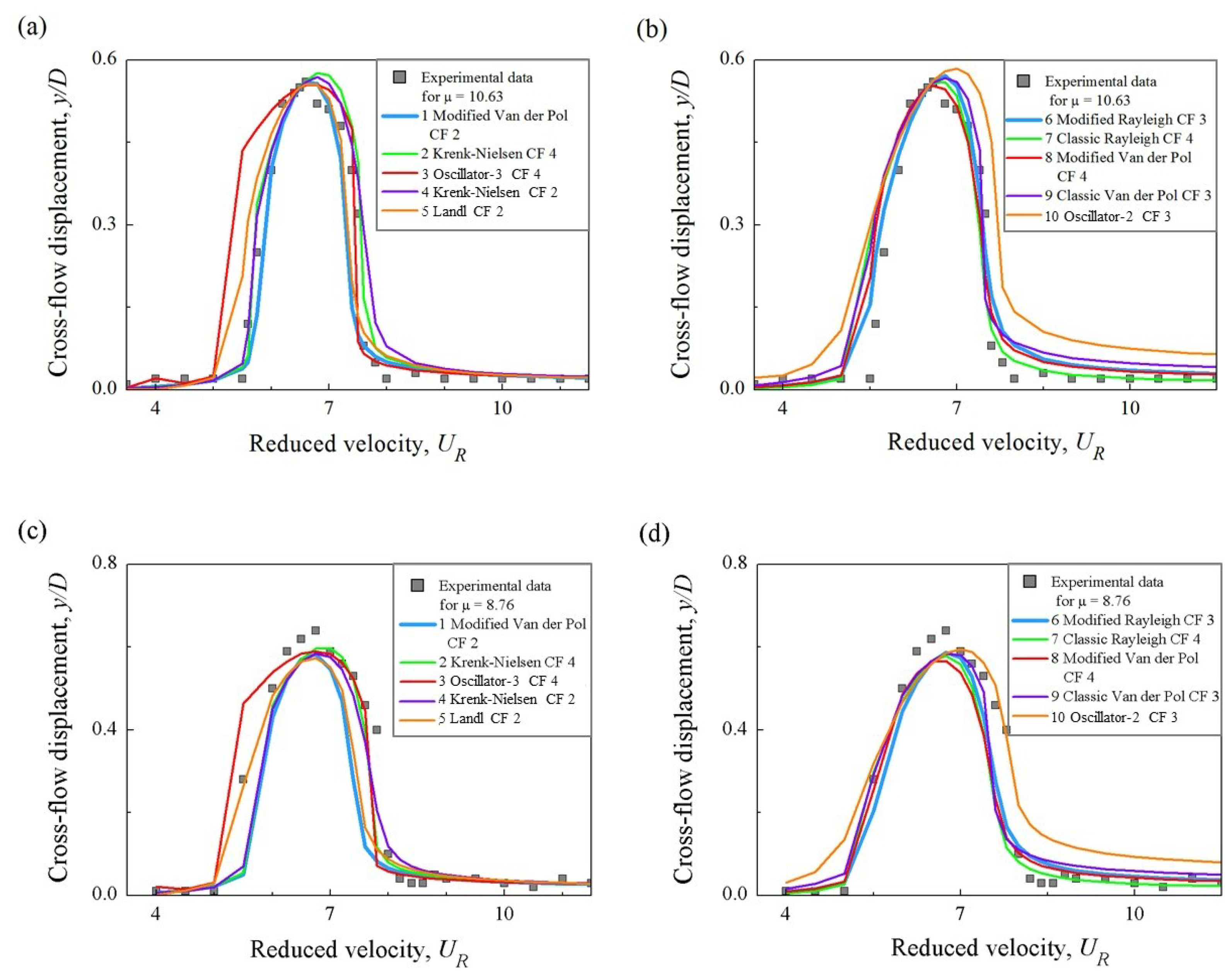
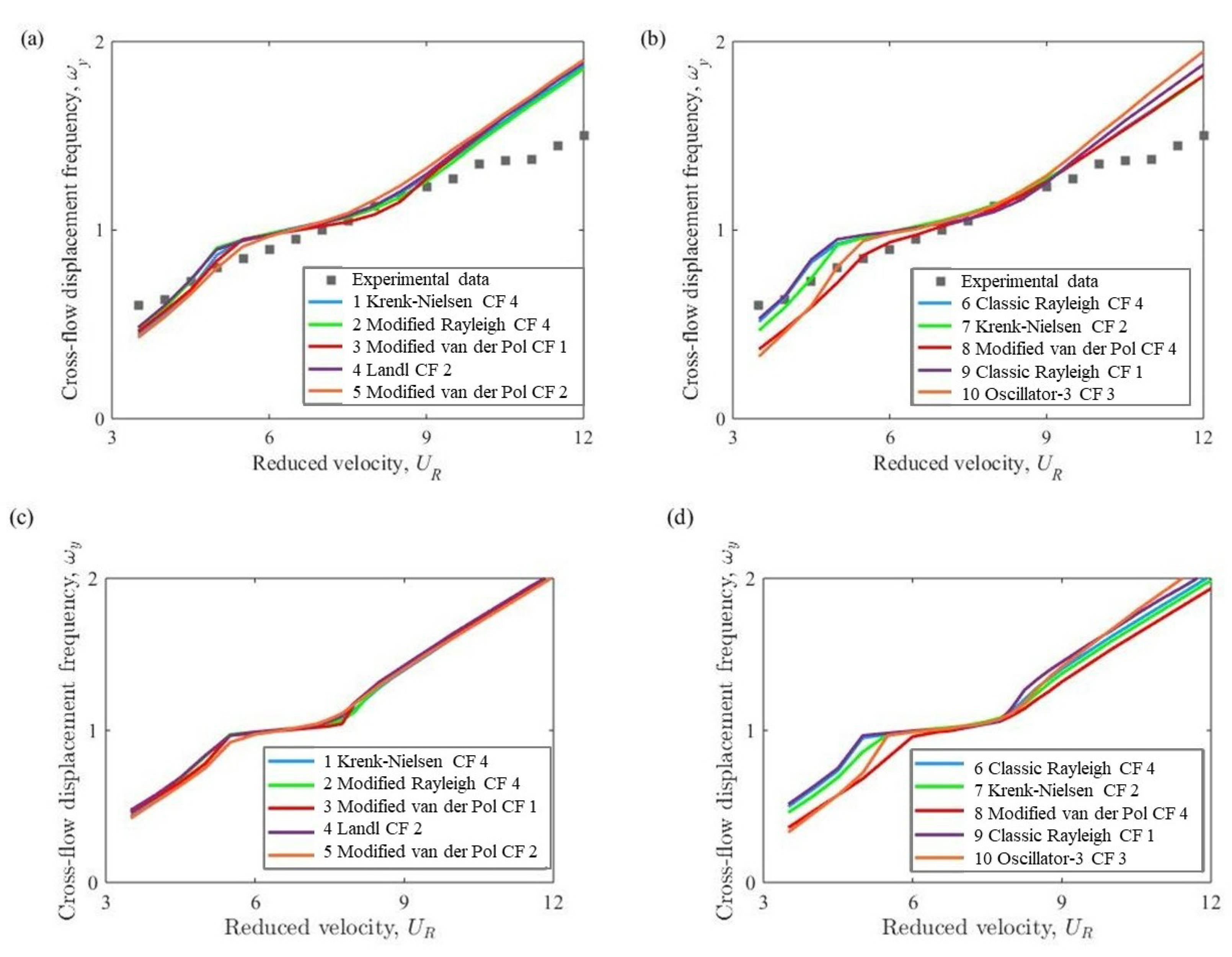
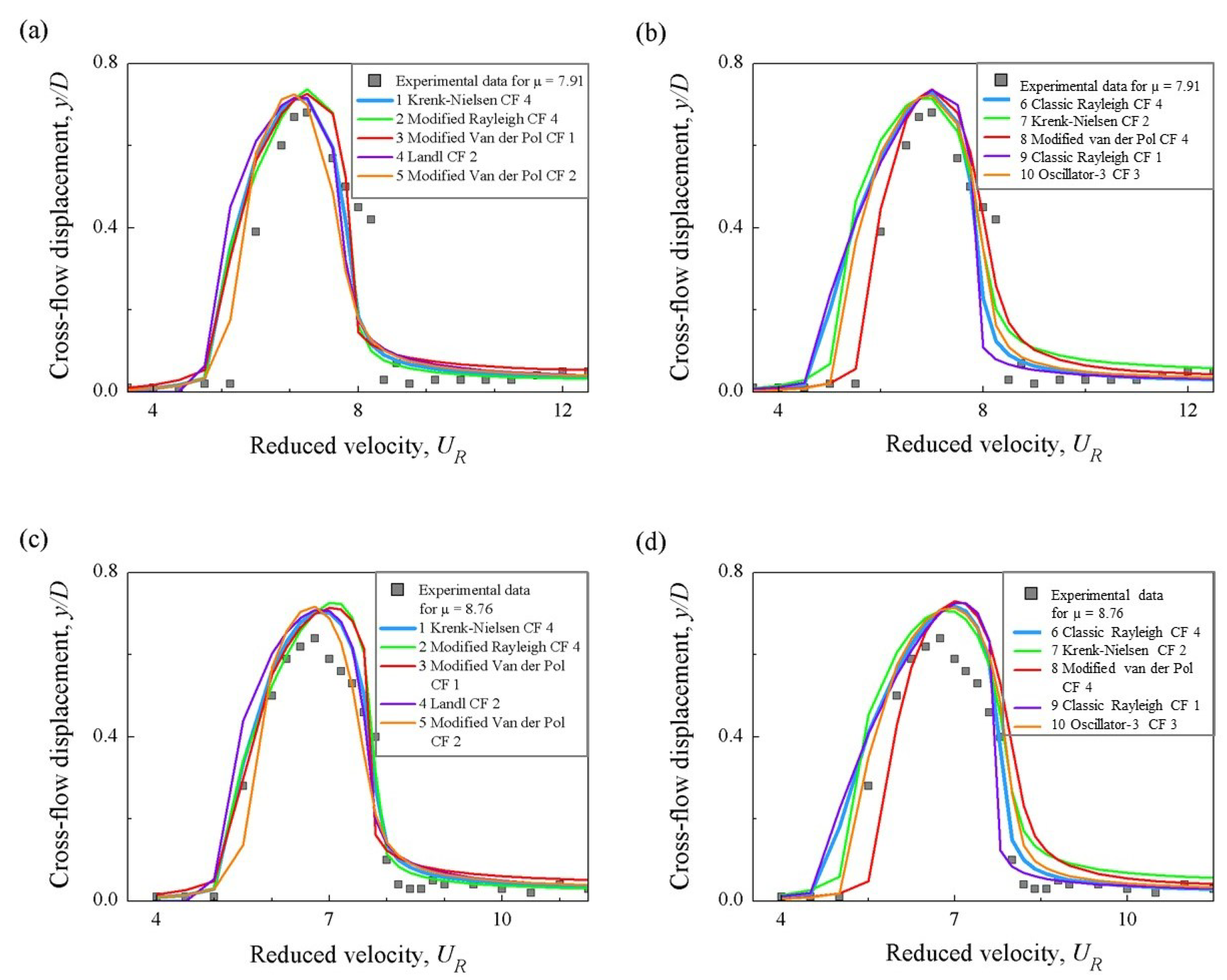
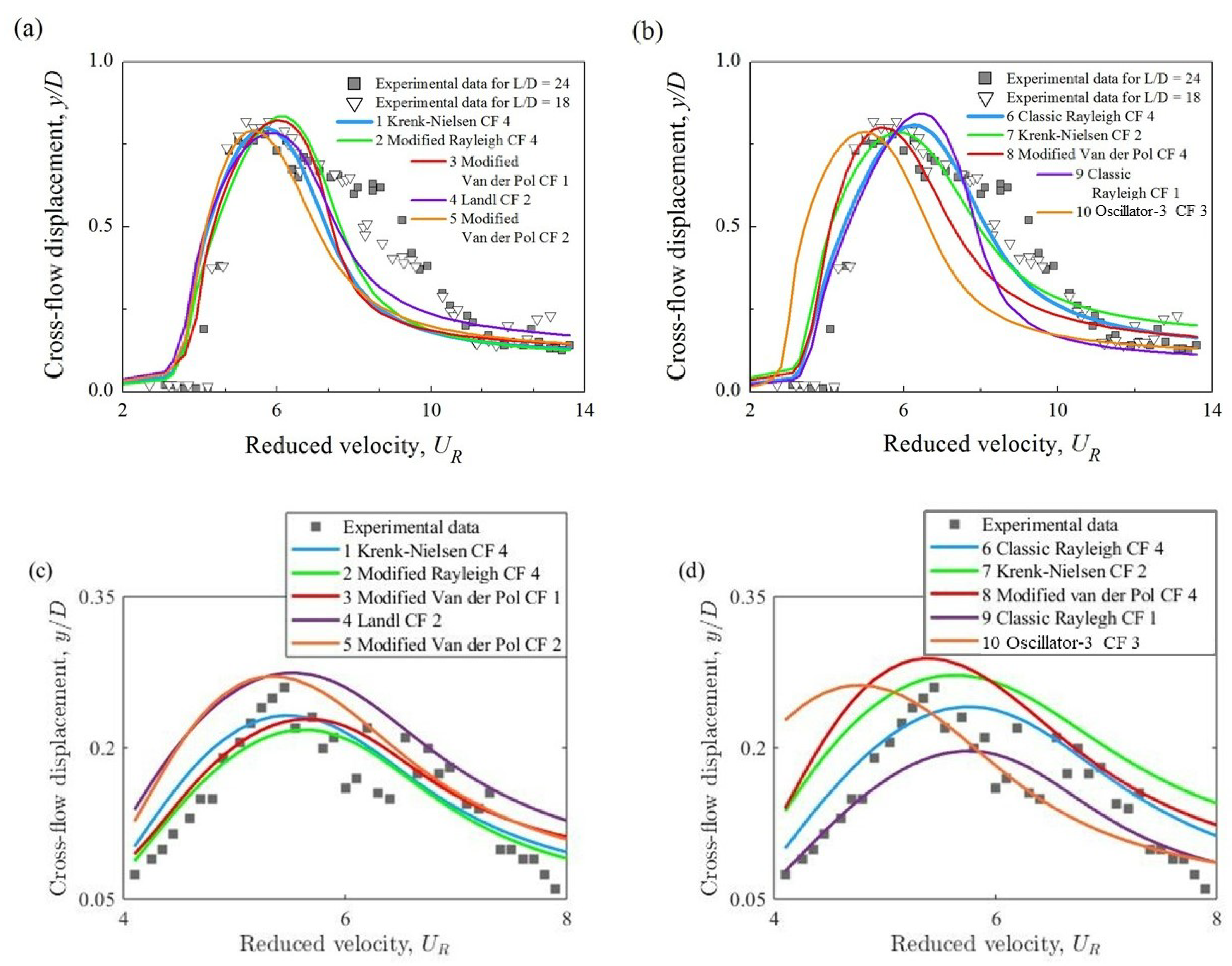
4.2. Models Calibrated with High Mass Ratio
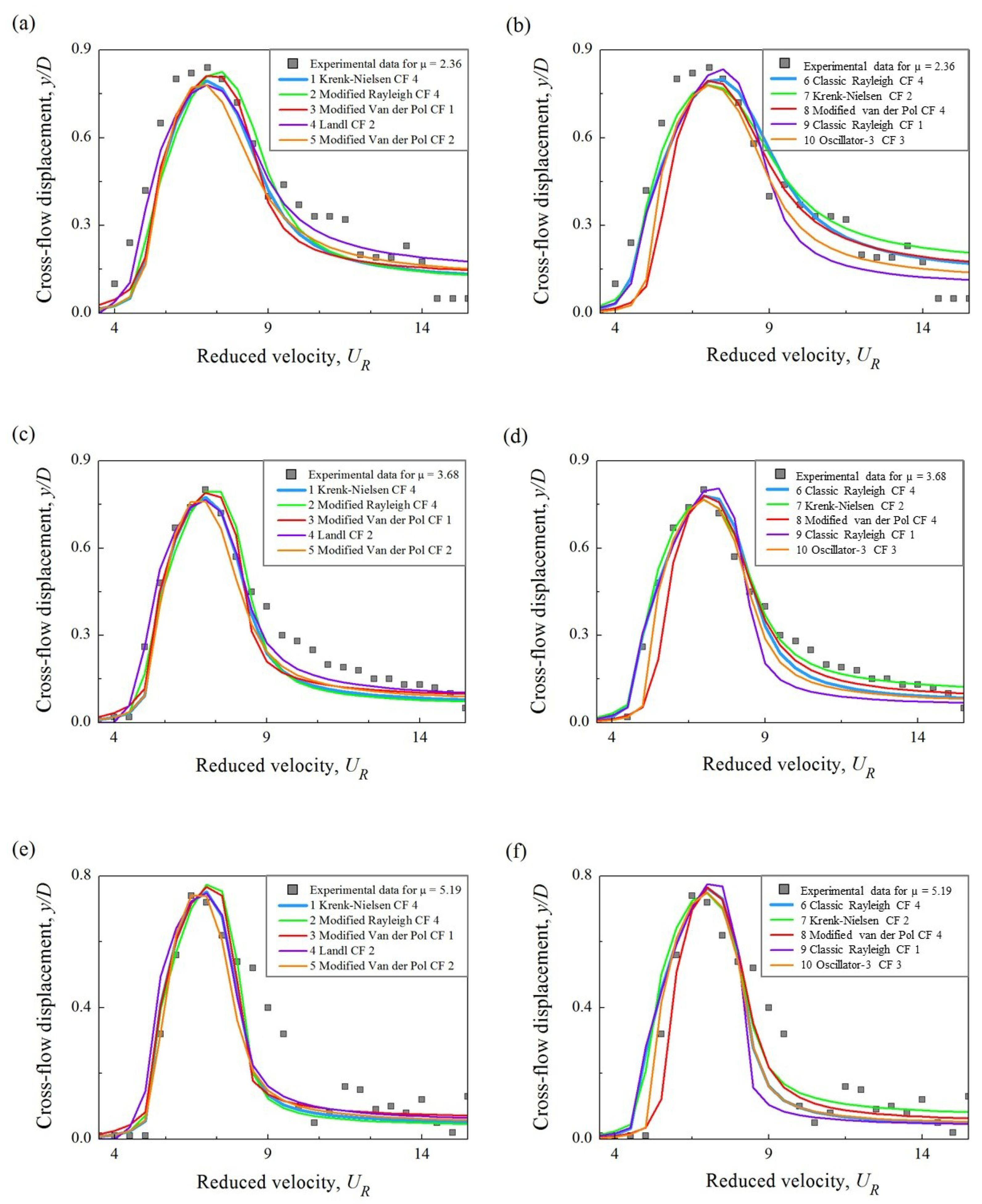
4.3. Models Calibrated with Medium Mass Ratio
4.4. Discussion
5. Conclusions
- General recommendation to fine-tune the phenomenological models with the data for a medium mass ratio around , which allows capturing features of the lock-in response for an extended mass ratio range.
- Advantageous use of the Krenk–Nielsen wake oscillator for cross-flow only VIV, compared to considered alternatives, including fluid oscillators with extended damping terms.
- Confirmed necessity to account for the lock-in occurrence sensitivity in terms of the reduced velocity and the related Reynolds number to the specific features of experimental arrangements (often associated with the physical boundary conditions), that can be achieved by the introduction of the vortex shedding frequency tuning parameter, named the lock-in delay coefficient in this work.
- General recommendation to model transversal-only oscillations with the models calibrated with the data for transverse VIV responses.
Author Contributions
Funding
Conflicts of Interest
Appendix A. Optimization Settings

| Parameter | Symbol | Initial Value | Lower Bound | Upper Bound |
|---|---|---|---|---|
| Initial lift coefficient | 0.3 | 0.01 | 3 | |
| Initial drag coefficient | 2 | 0.01 | 3 | |
| Cross-flow fluid damping parameter | 0.008 | 0.00001 | 2 | |
| Coupling coefficient | 5 | 0 | 40 | |
| Fluid added mass coefficient | 1 | 0.1 | 2 | |
| Lock-in delay coefficient | K | 0 | 0 | 4 |
Appendix B. Optimized Coefficients
| Fluid Oscillator | Objective Function | K | |||||
|---|---|---|---|---|---|---|---|
| Low Mass Ratio | |||||||
| 1. Classic Rayleigh | CF 3 | 0.75 | 2.25 | 0.006424 | 4.98 | 0.72 | 0.95 |
| 2. Classic Rayleigh | CF 4 | 0.80 | 2.23 | 0.008998 | 5.12 | 0.91 | 0.94 |
| 3. Classic van der Pol | CF 2 | 0.66 | 2.57 | 0.050361 | 7.48 | 1.50 | 1.17 |
| 4. Modified van der Pol | CF 1 | 0.74 | 1.41 | 0.358890, 0.547880 | 3.63 | 0.70 | 0.85 |
| 5. Modified Rayleigh | CF 3 | 0.47 | 1.81 | 0.009570, 0.399190 | 5.02 | 0.93 | 0.75 |
| 6. Modified van der Pol | CF 2 | 0.37 | 1.90 | 0.025168, 0.332520 | 5.98 | 0.65 | 1.06 |
| 7. Classic van der Pol | CF 1 | 0.88 | 1.80 | 0.295900 | 4.56 | 0.85 | 0.85 |
| 8. Modified Rayleigh | CF 4 | 0.84 | 2.25 | 0.022750, 0.223730 | 5.73 | 1.56 | 0.74 |
| 9. Krenk–Nielsen | CF 4 | 0.89 | 2.24 | 0.019919, 0.033541, 0.008071 | 5.11 | 0.78 | 1.01 |
| 10. Oscillator-4 | CF 2 | 0.33 | 1.97 | 0.171950, 0.009893, 0.003658, | 11.10 | 0.69 | 1.22 |
| 0.006449, 0.000965, 0.000248, | |||||||
| 0.000068, 0.001285, 0.000001, | |||||||
| 0.000018, 0.000009, 0.000003, | |||||||
| 0.000019, 0.000118 | |||||||
| Medium Mass Ratio | |||||||
| 1. Krenk–Nielsen | CF 4 | 0.61 | 1.75 | 0.081990, 0.016313, 0.012551 | 5.49 | 1.12 | 1.34 |
| 2. Modified Rayleigh | CF 4 | 0.69 | 1.70 | 0.016162, 0.038019 | 5.14 | 0.95 | 1.22 |
| 3. Modified van der Pol | CF 1 | 0.58 | 1.22 | 0.367820, 0.696500 | 3.85 | 0.97 | 1.17 |
| 4. Landl | CF 2 | 0.67 | 1.90 | 0.008562, 0.009240, 0.008891 | 5.08 | 1.00 | 1.17 |
| 5. Modified van der Pol | CF 2 | 0.48 | 2.22 | 0.026508, 0.035601 | 6.28 | 1.13 | 1.40 |
| 6. Classic Rayleigh | CF 4 | 0.84 | 2.03 | 0.019019 | 5.28 | 0.87 | 1.04 |
| 7. Krenk–Nielsen | CF 2 | 0.86 | 2.03 | 0.177330, 0.088756, 0.036305 | 5.16 | 1.01 | 1.23 |
| 8. Modified van der Pol | CF 4 | 0.75 | 2.41 | 0.029661, 0.027102 | 4.65 | 1.12 | 1.70 |
| 9. Classic Rayleigh | CF 1 | 0.82 | 1.55 | 0.080460 | 4.71 | 1.19 | 0.96 |
| 10. Oscillator-3 | CF 3 | 0.79 | 2.71 | 0.048490, 0.030415, 0.011808, | 9.42 | 1.68 | 2.12 |
| 0.017899, 0.381170, 0.010902, | |||||||
| 0.000964, 0.001431, 0.000161 | |||||||
| High Mass Ratio | |||||||
| 1. Modified van der Pol | CF 2 | 0.39 | 1.42 | 0.057390, 0.075106 | 4.68 | 0.78 | 1.43 |
| 2. Krenk–Nielsen | CF 4 | 0.46 | 1.32 | 0.144630, 0.029808, 0.012312 | 5.53 | 1.30 | 1.44 |
| 3. Oscillator-3 | CF 4 | 0.40 | 0.70 | 1.974500, 0.001903, 0.028620, | 19.31 | 0.75 | 2.32 |
| 0.126120, 0.573010, 0.067134, | |||||||
| 0.032737, 0.094681, 0.058406 | |||||||
| 4. Krenk–Nielsen | CF 2 | 0.62 | 2.04 | 0.050086, 0.045857, 0.014756 | 5.21 | 1.92 | 1.46 |
| 5. Landl | CF 2 | 0.64 | 1.74 | 0.000104, 0.000065, 0.014635 | 3.95 | 0.99 | 1.26 |
| 6. Modified Rayleigh | CF 3 | 0.50 | 1.65 | 0.007572, 0.023123 | 4.92 | 0.58 | 1.39 |
| 7. Classic Rayleigh | CF 4 | 0.67 | 2.04 | 0.010910 | 4.95 | 0.99 | 1.16 |
| 8. Modified van der Pol | CF 4 | 0.58 | 2.01 | 0.043130, 0.071177 | 5.10 | 0.77 | 1.28 |
| 9. Classic van der Pol | CF 3 | 1.12 | 1.45 | 0.654710 | 2.05 | 1.00 | 1.10 |
| 10. Oscillator-2 | CF 3 | 0.37 | 2.51 | 0.009732, 0.010817, 0.000125, | 10.05 | 1.15 | 1.25 |
| 0.014392, 0.013879, 0.000637 |
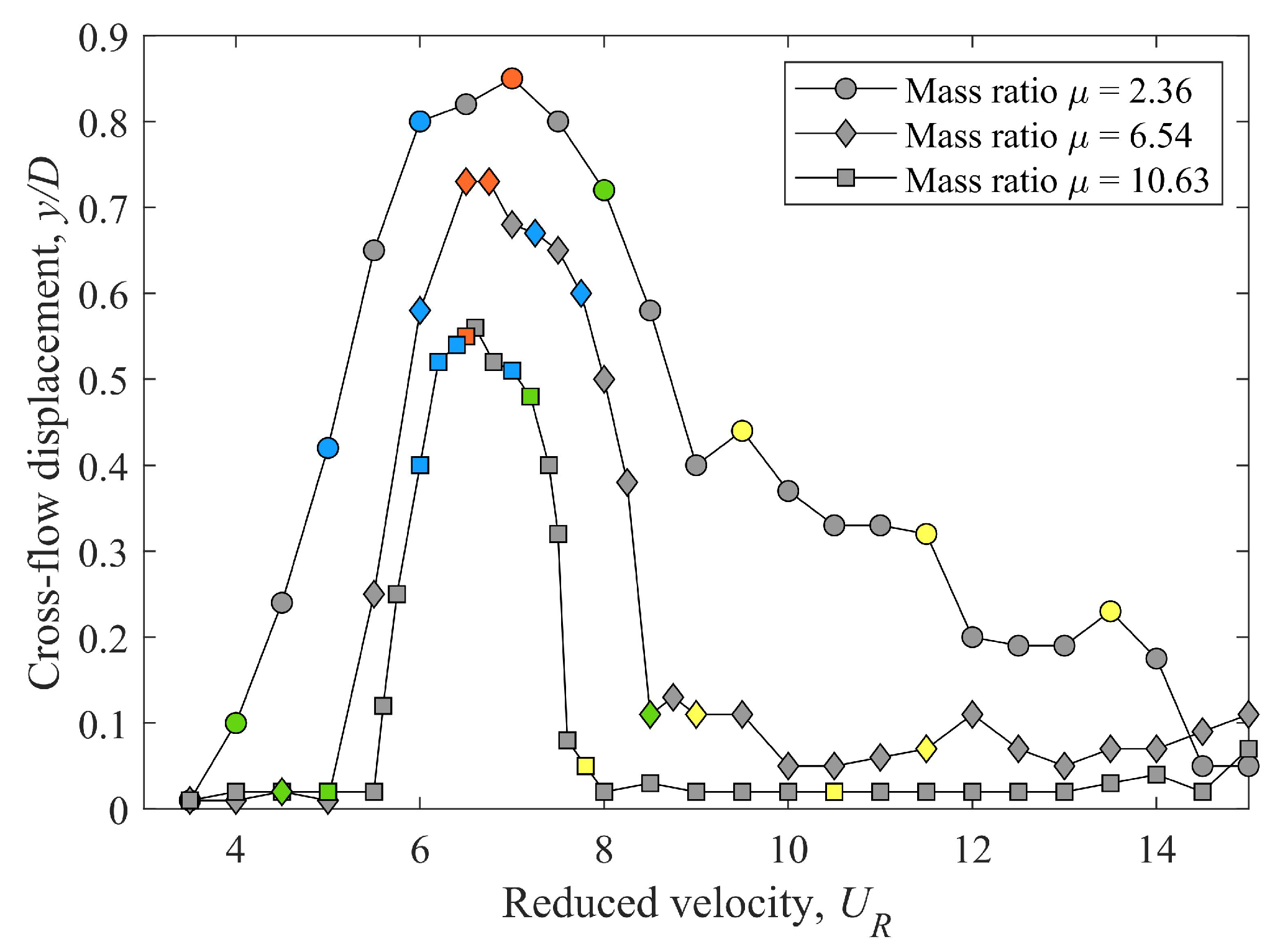
Appendix C. Experimental Case Parameters
| Parameter, Symbol (Units) | Value | ||
|---|---|---|---|
| Experimental Set-Up | Stappenbelt and O’Neill (2007) [32] | Franzini et al. (2009) [33] | Blevins and Coughran (2009) [34] |
| Mass ratio, | |||
| Damping ratio, | |||
| Mass-damping ratio, | |||
| Griffin mass-damping | |||
| ratio, | |||
| Maximum lock-in displacement | , | ||
| amplitude, | |||
| Diameter, D (m) | |||
| Aspect ratio, | 8 | 18, 24 | |
| Natural frequency of structure, (Hz) | |||
| Flow velocity interval, U (m/s) | 0.20–0.96 | 0.042–0.209 | 0.31–0.61 |
| Reynolds number interval, | 10,810–52,560 | 1320–6660 | 19,890–39,050 |
| Reduced velocity interval, | 3.4–14.3 | 2.7–13.6 | 4.10–8.05 |
References
- Hartlen, R.; Currie, I. Lift-oscillator model of vortex-induced vibration. J. Eng. Mech. Div. 1970, 96, 577–591. [Google Scholar] [CrossRef]
- Skop, R.; Griffin, O. A model for vortex-excited resonance response of bluff cylinders. J. Sound Vib. 1973, 27, 225–233. [Google Scholar] [CrossRef]
- Landl, R. A mathematical model for vortex-excited vibrations of bluff bodies. J. Sound Vib. 1975, 42, 219–234. [Google Scholar] [CrossRef]
- Skop, R.; Griffin, O. On a theory for the vortex-excited oscillations of flexible cylindrical structures. J. Sound Vib. 1975, 41, 263–274. [Google Scholar] [CrossRef]
- Srinil, N.; Zanganeh, H. Modelling of coupled cross-flow/in-line vortex-induced vibrations using double Duffing and van der Pol oscillators. Ocean Eng. 2012, 53, 83–97. [Google Scholar] [CrossRef] [Green Version]
- Krenk, S.; Nielsen, S. Energy balanced double oscillator model for vortex-induced vibrations. J. Eng. Mech. 1999, 125, 263–271. [Google Scholar] [CrossRef]
- Ogink, R.; Metrikine, A. A wake oscillator with frequency dependent tuning coefficients for the modeling of VIV. In Proceedings of the ASME 2008 27th International Conference on Offshore Mechanics and Arctic Engineering, Estoril, Portugal, 15–20 June 2008; pp. 943–952. [Google Scholar]
- Kurushina, V.; Pavlovskaia, E. Wake oscillator equations in modelling vortex-induced vibrations at low mass ratios. In Proceedings of the OCEANS 2017, Aberdeen, UK, 19–22 June 2017; pp. 1–6. [Google Scholar]
- Shoshani, O. Deterministic and stochastic analyses of the lock-in phenomenon in vortex-induced vibration. J. Sound Vib. 2018, 434, 17–27. [Google Scholar] [CrossRef]
- Wang, J.; Fu, S.; Baarholm, R.; Wu, J.; Larsen, C. Fatigue damage induced by vortex-induced vibrations in oscillatory flow. Mar. Struct. 2015, 40, 73–91. [Google Scholar] [CrossRef]
- Facchinetti, M.; De Langre, E.; Biolley, F. Coupling of structure and wake oscillators in vortex-induced vibrations. J. Fluids Struct. 2004, 19, 123–140. [Google Scholar] [CrossRef]
- Ogink, R.; Metrikine, A. A wake oscillator with frequency dependent coupling for the modeling of vortex-induced vibration. J. Sound Vib. 2010, 329, 5452–5473. [Google Scholar] [CrossRef]
- Qu, Y.; Metrikine, A. A Wake Oscillator Model With Nonlinear Coupling for the VIV of Rigid Cylinder Constrained to Vibrate in the Cross-Flow Direction. In Proceedings of the ASME 2016 35th International Conference on Ocean, Offshore and Arctic Engineering, Busan, Korea, 19–24 June 2016; Volume 49934, p. V002T08A037. [Google Scholar]
- Qu, Y.; Metrikine, A. A wake oscillator model with nonlinear coupling for the vortex-induced vibration of a rigid cylinder constrained to vibrate in the cross-flow direction. J. Sound Vib. 2020, 469, 115161. [Google Scholar] [CrossRef]
- Nayfeh, A.; Owis, F.; Hajj, M. A model for the coupled lift and drag on a circular cylinder. In Proceedings of the ASME 2003 International Design Engineering Technical Conferences and Computers and Information in Engineering Conference, Chicago, IL, USA, 2–6 September 2003; pp. 1289–1296. [Google Scholar]
- Barbosa, J.; Qu, Y.; Metrikine, A.; Lourens, E.M. Vortex-induced vibrations of a freely vibrating cylinder near a plane boundary: Experimental investigation and theoretical modelling. J. Fluids Struct. 2017, 69, 382–401. [Google Scholar] [CrossRef] [Green Version]
- Qu, Y.; Metrikine, A. A single van der Pol wake oscillator model for coupled cross-flow and in-line vortex-induced vibrations. Ocean Eng. 2020, 196, 106732. [Google Scholar] [CrossRef]
- Stappenbelt, B.; Lalji, F. Vortex-induced vibration super-upper response branch boundaries. Int. J. Offshore Polar Eng. 2008, 18, 99–105. [Google Scholar]
- Postnikov, A. Wake Oscillator and CFD in Modelling of VIVs. Ph.D. Thesis, University of Aberdeen, Aberdeen, UK, 2016. [Google Scholar]
- Srinil, N.; Opinel, P.A.; Tagliaferri, F. Empirical sensitivity of two-dimensional nonlinear wake–cylinder oscillators in cross-flow/in-line vortex-induced vibrations. J. Fluids Struct. 2018, 83, 310–338. [Google Scholar] [CrossRef] [Green Version]
- Kinaci, O.; Lakka, S.; Sun, H.; Bernitsas, M. Effect of tip-flow on vortex-induced vibration of circular cylinders. Ocean Eng. 2016, 117, 130–142. [Google Scholar] [CrossRef] [Green Version]
- Kurushina, V.; Pavlovskaia, E.; Postnikov, A.; Wiercigroch, M. Calibration and comparison of VIV wake oscillator models for low mass ratio structures. Int. J. Mech. Sci. 2018, 142, 547–560. [Google Scholar] [CrossRef] [Green Version]
- Blevins, R.; Coughran, C. Experimental investigation of vortex-induced vibration in two-dimensions. In Proceedings of the Eighteenth International Offshore and Polar Engineering Conference, Vancouver, BC, Canada, 6–11 July 2008; International Society of Offshore and Polar Engineers: Mountain View, CA, USA, 2008. [Google Scholar]
- Dahl, J.; Hover, F.; Triantafyllou, M. Two-degree-of-freedom vortex-induced vibrations using a force assisted apparatus. J. Fluids Struct. 2006, 22, 807–818. [Google Scholar] [CrossRef]
- Jauvtis, N.; Williamson, C. The effect of two degrees-of-freedom on vortex-induced vibration at low mass and damping. J. Fluid Mech. 2004, 509, 23–62. [Google Scholar] [CrossRef]
- Kurushina, V.; Pavlovskaia, E. Fluid nonlinearities effect on wake oscillator model performance. Matec Web Conf. 2018, 148, 04002. [Google Scholar] [CrossRef] [Green Version]
- Kurushina, V.; Pavlovskaia, E.; Wiercigroch, M. VIV of flexible structures in 2D uniform flow. Int. J. Eng. Sci. 2020, 150, 103211. [Google Scholar] [CrossRef]
- Kurushina, V.; Pavlovskaia, E.; Postnikov, A.; Franzini, G.R.; Wiercigroch, M. Modelling VIV of Transversally Oscillating Rigid Structures Using Nonlinear Fluid Oscillators. In Nonlinear Dynamics of Structures, Systems and Devices; Springer: Berlin/Heidelberg, Germany, 2020; pp. 379–387. [Google Scholar]
- Postnikov, A.; Pavlovskaia, E.; Wiercigroch, M. 2DOF CFD calibrated wake oscillator model to investigate vortex-induced vibrations. Int. J. Mech. Sci. 2017, 127, 176–190. [Google Scholar] [CrossRef] [Green Version]
- Govardhan, R.; Williamson, C. Modes of vortex formation and frequency response of a freely vibrating cylinder. J. Fluid Mech. 2000, 420, 85–130. [Google Scholar] [CrossRef]
- Blevins, R. Flow-Induced Vibration; Van Nostrand Reinhold Co., Inc.: New York, NY, USA, 1990. [Google Scholar]
- Stappenbelt, B.; O’Neill, L. Vortex-induced vibration of cylindrical structures with low mass ratio. In Proceedings of the Seventeenth International Offshore and Polar Engineering Conference, Lisbon, Portugal, 1–6 July 2007. [Google Scholar]
- Franzini, G.; Fujarra, A.; Meneghini, J.; Korkischko, I.; Franciss, R. Experimental investigation of vortex-induced vibration on rigid, smooth and inclined cylinders. J. Fluids Struct. 2009, 25, 742–750. [Google Scholar] [CrossRef]
- Blevins, R.; Coughran, C. Experimental investigation of vortex-induced vibration in one and two dimensions with variable mass, damping, and Reynolds number. J. Fluids Eng. 2009, 131, 101202. [Google Scholar] [CrossRef]
- Govardhan, R.; Williamson, C. Mean and fluctuating velocity fields in the wake of a freely-vibrating cylinder. J. Fluids Struct. 2001, 15, 489–501. [Google Scholar] [CrossRef]
- Kurushina, V. Fluid Nonlinearities for Calibrated VIV Wake Oscillator Models. Ph.D. Thesis, University of Aberdeen, Aberdeen, UK, 2018. [Google Scholar]


| Oscillator | Cross-Flow Equation |
|---|---|
| Classic van der Pol | |
| Modified van der Pol | |
| Classic Rayleigh | |
| Modified Rayleigh | |
| Landl | |
| Krenk–Nielsen | |
| Oscillator-1 | |
| Oscillator-2 | |
| Oscillator-3 | |
| Oscillator-4 | |
| Parameter, Symbol (Units) | Value |
|---|---|
| Mass ratio, | |
| Damping ratio, | |
| Mass-damping ratio, | |
| Griffin mass-damping | |
| ratio, | |
| Maximum lock-in displacement | |
| amplitude, | |
| Diameter, D (m) | |
| Aspect ratio, | 8 |
| Natural frequency, (Hz) | |
| Flow velocity interval, U (m/s) | 0.33–1.52 |
| Reynolds number interval, | 18,300–83,800 |
| Reduced velocity interval, | 3.5–16.0 |
| Number | Objective Function |
|---|---|
| CF 1 | |
| CF 2 | |
| CF 3 | |
| CF 4 |
| Mass Ratio | Borders of Application on the Same Set-Up in Terms of Mass Ratio | Borders of Application on Different Experimental Set-Ups in Terms of Mass Ratio |
|---|---|---|
| 1DOF | ||
| Low | From 2 to 5, including | From 2 to 5, excluding |
| lock-in delay coefficient | lock-in delay coefficient | |
| Medium | From 2-3 to 10-11, including | From 2 to 5, excluding |
| lock-in delay coefficient | lock-in delay coefficient | |
| High | From 9 to 11, including | - |
| lock-in delay coefficient | ||
| 2DOF | ||
| Low | From 2 to 5, including | From 2 to 4, including |
| lock-in delay coefficient | lock-in delay coefficient | |
| Medium | From 2 to 10, including | - |
| lock-in delay coefficient | ||
| High | From 9 to 11, including | - |
| lock-in delay coefficient | ||
Publisher’s Note: MDPI stays neutral with regard to jurisdictional claims in published maps and institutional affiliations. |
© 2022 by the authors. Licensee MDPI, Basel, Switzerland. This article is an open access article distributed under the terms and conditions of the Creative Commons Attribution (CC BY) license (https://creativecommons.org/licenses/by/4.0/).
Share and Cite
Kurushina, V.; Postnikov, A.; Franzini, G.R.; Pavlovskaia, E. Optimization of the Wake Oscillator for Transversal VIV. J. Mar. Sci. Eng. 2022, 10, 293. https://doi.org/10.3390/jmse10020293
Kurushina V, Postnikov A, Franzini GR, Pavlovskaia E. Optimization of the Wake Oscillator for Transversal VIV. Journal of Marine Science and Engineering. 2022; 10(2):293. https://doi.org/10.3390/jmse10020293
Chicago/Turabian StyleKurushina, Victoria, Andrey Postnikov, Guilherme Rosa Franzini, and Ekaterina Pavlovskaia. 2022. "Optimization of the Wake Oscillator for Transversal VIV" Journal of Marine Science and Engineering 10, no. 2: 293. https://doi.org/10.3390/jmse10020293