Short-Term Variations in Water Temperature of the Antarctic Surface Layer

Abstract

Against the background of global climate change, the warming water temperature of Antarctic surface water (<500 m) is worthy of study. Therefore, the purpose of this study was to investigate short-term variations in the water temperature of Antarctic surface water from January 2000 to December 2016, using offline coupled ocean models, i.e., the WAVEWATCH-III (WW3) model and the Stony Brook Parallel Ocean Model (sbPOM). The validation of the WW3-simulated significant wave height (SWH) against the measurements from the Jason-2 altimeter produced a root mean square error (RMSE) of 0.39 m with a 0.30-m bias. Moreover, the sbPOM-simulated water temperatures were compared with the collocated measurements from Argo buoys, yielding, and RMSE for water temperatures of less than 1.0 °C and a correlation coefficient (COR) of 0.92. The annual variation in the sbPOM-simulated water temperatures of the Antarctic surface water layer showed that the sea surface temperatures (SSTs) of the Pacific Ocean and Atlantic Ocean were greater than the SST of the Indian Ocean. Moreover, the SST rapidly increased to 2 °C in the Pacific Ocean in specific years due to El Nino and La Nina events. The vertical profile of the water temperature showed that the depth of the cool water in the Indian Ocean has decreased to 100 m since 2008, while the depth in the Pacific Ocean and Atlantic Ocean is about 200 m. It was also found that the seasonal variations in the water temperature at depths of 0 m, 50 m, and 100 m in the Pacific Ocean were more sensitive to El Nino events between January and June. However, it was revealed in this work that the increasing intensity of El Nino and La Nina events could reduce water warming in the Pacific Ocean.

1. Introduction

In the last few decades, the sea ice in the Arctic and Antarctic oceans has significantly and gradually melted [1,2], changing with the variations in the global climate, due to the correlations between the detrended sea ice edge anomaly and various climatic factors [3]. Specifically, variations in the water temperature [4] and sea fetch, which are affected by the reduction in the amount of sea ice in the Antarctic Ocean, have significant influences on the movement of ocean waves [5] and circulation [6]. The characteristics of ocean dynamics are complicated in the open sea areas of the Antarctic Ocean, e.g., the circumpolar current [7] and huge swells [8]. In fact, both the currents and waves play important roles in water temperature [9], especially under the high sea state in the Antarctic Ocean. However, regarding the oceanography research conducted on the Antarctic Ocean, the characteristics of the atmospheric–marine dynamics and climate change, i.e., wind [10], waves [11], and currents [12], have been individually studied. Moreover, variations in water temperature are sensitive to global climate change [13], e.g., the warming of the Antarctic surface and bottom water.

Techniques for sea surface observations in previous studies included moored buoys and remote sensing techniques. However, the measurements from buoys and remote-sensed data measurements are expensive, and it is not easy to obtain long-term continuous observations. With the development of oceanographic theories and computation techniques, several numerical ocean models have been proposed for sea surface waves and ocean circulation simulations. The third-generation numerical wave ocean model (WAM), based on the evolution of a two-dimensional ocean wave spectrum, was initially developed by the WAMDIG group [14] in the 1980s. Recently, two third-generation wave models, i.e., the WAVEWATCH-III (WW3) [15] and Simulation Wave Nearshore (SWAN) [16] models, have become popular for wave analysis, especially under extreme sea states [17]. The SWAN model involves the implementation of unstructured grids in its computation, which satisfies the requirements for coast lines, while structured grids are employed in the WW3 model, allowing for wave simulation over regional [18] and global seas [19]. In particular, the WW3 model is usually used for wave analysis in polar regions because it includes several switches that consider ice–wave interactions. In our recent study [5], the inclusion of sea ice in wave simulations using eight parametric switches in the WW3 model (version 6.07) was investigated, and it was found that the switch denoted as IC4_M1 [20] had the most effective performance (root mean square error (RMSE) of 0.68 m) in high latitude regions (60–80° N).

Ocean circulation simulations are more complicated than wave simulations, due to the vertical baroclinic characteristic of sea water. It should be noted that the original code for the POM is conveniently modifiable for operational applications in sensitive experiments. Moreover, studies carried out on typhoons [21] have concluded that the POM has the capability to illustrate the cooling of the sea surface temperature (SST) and to simulate the summer circulation structure in the South China Sea well [22]. The improvement of the parallel version of the POM, i.e., the Stony Brook Parallel Ocean Model (sbPOM) [23], increased computational efficiency, and it is now available to public users for scientific purposes. In our recent study, four wave-induced terms, i.e., breaking waves, nonbreaking waves, radiation stress, and Stokes drift, were included in the water temperature simulation by sbPOM in order to study the SST cooling in tropical cyclones [24].

In the context of global change, the distribution of the sea temperature is affected by the input of shelf meltwater in the Antarctic Ocean. The impact of sea-ice in the Antarctic Ocean on the SST in the Indian Ocean and the warming of the Antarctic bottom water has been well studied [25,26]; however, variations in the temperature of Antarctic surface water (<500 m) are worthy of investigation, especially for entire Oceans, e.g., the Pacific Ocean, the Atlantic Ocean and the Indian Ocean. In particular, the water temperature simulation should consider the influence of the waves under the high sea state in the Antarctic Ocean. The current data from the National Centers for Environmental Prediction (NCEP) Climate Forecast System Version 2 (CFSv2) were used as the open boundary conditions in the wave simulation using the WW3 model. Four wave-induced terms, i.e., breaking waves, nonbreaking waves, radiation stress, and Stokes drift, were included in the water temperature simulation using the sbPOM; however, we have not implemented the spin-up for WW3 and sbPOM, as the simulation lasts for 16 years. The purpose of this study was to investigate the short-term variability of the water temperature in the Antarctic Ocean during the period from January 2000 to December 2016 by using offline coupled ocean models, i.e., WW3 and sbPOM. Specifically, the water warming of the Antarctic surface layer (<500 m), the Pacific Ocean, the Atlantic Ocean and the Indian Ocean were investigated in the context of El Nino and La Nina events. The data and the settings for the WW3 and sbPOM are introduced in detail in the Materials and Methods section. The calculation of the four terms induced by waves, which were derived from WW3 simulations, is also presented in this section. The accuracy of the water temperature simulation using the sbPOM and the variations in temperature in the Antarctic Ocean are presented in the Results section, and the Discussion section presents the characteristics of Antarctic surface water in El Nino and La Nina events. The conclusions are summarized in the Conclusions section.

2. Materials and Methods

In this section, the basic descriptions of the two numeric models, i.e., WW3 and sbPOM, and the model settings, are briefly introduced. In particular, the method of introducing four terms induced by sea surface waves in the sbPOM is described.

2.1. Model Settings of WW3

In principle, the simulation of the waves using the WW3 model is conducted by solving the wave propagation balance equation [15]:

$$\frac{\mathrm{D}}{{\mathrm{D}}_{\mathrm{t}}}\left(\mathrm{F}\left(\mathrm{k},\mathsf{\theta };\mathrm{x},\mathrm{t}\right)\right)=\frac{\mathrm{S}(\mathrm{k},\mathsf{\theta };\mathrm{x},\mathrm{t})}{\mathsf{\sigma }},$$

(1)

where D and D_t represent partial derivatives.

$${\mathrm{S}=\mathrm{S}}_{\mathrm{in}}{ + \mathrm{S}}_{\mathrm{bot}}{ + \mathrm{S}}_{\mathrm{db} }{ + \mathrm{S}}_{\mathrm{nl}}{ + \mathrm{S}}_{\mathrm{tq}},$$

(2)

in which F is the wave action density spectrum, S includes the input and dissipation source terms, k is the wave number, θ is the wave propagation direction, σ is the intrinsic frequency, and x and t are the space and time coordinates, respectively. Typically, S is the sum of the wind-generated energy S_in in the air–sea boundary layer; the friction induced by the wave–bottom interactions is S_bot; the dissipation caused by breaking waves is S_db; the non-linear component due to wave–wave interactions is indicated by S_nl; and the multiple wave–wave (three and four waves) interaction term is S_tq.

In this study, the computing region of the two ocean models in the Antarctic Ocean was between (49.75° N, 0° E) and (49.75° N, 360° E) with a rectangle grid of 0.25°. Because the detailed parametrizations of these terms are provided in the technical manual for the WW3 model [27,28], we briefly state the settings, as shown in

Table 1. The basic settings for the WAVEWATCH-III (WW3) model and the Stony Brook Parallel Ocean Model (sbPOM).

	Forcing Fields	Output Resolution
WAVEWATCH-III (WW3)	The European Centre for Medium-Range Weather Forecast (ECMWF) data; the National Centers for Environmental Prediction (NCEP) Climate Forecast System Version 2 (CFSv2)	Temporal resolution of 1 h and spatial grid resolution of 0.25°
Stony Brook Parallel Ocean Model (sbPOM)	The European Centre for Medium-Range Weather Forecast (ECMWF) data; Simple Ocean Data Assimilation (SODA) sea surface temperature and salinity Wave-induced: breaking wave; nonbreaking wave Radiation stress; stokes drift; National Centers for Environmental Prediction (NCEP) latent heat flux; NCEP sensible heat flux; NCEP long-wave radiation; NCEP short-wave radiation;	Temporal resolution of 1 h and spatial grid resolution of 0.25°

. The parametrization of the input/dissipation terms was switch ST2+STAB2 [29]; switch GMD2 was used for the four wave–wave interactions [30]; switch IC4_M1 was used for the ice–wave interactions [5]; and the outputs were the wave parameters in 0.25° grids at a 1-h interval. That is, the significant wave height (SWH), peak wavelength, and mean wave period were used to calculate the four terms induced by waves.

2.2. The Data Used in WW3

Figure 1 shows the map of the computing domains for WW3 and sbPOM, overlaid with the 0.1° gridded water depth map from the GEBCO, which was spatially interpolated to 1 km during the modeling process. The Antarctic Ocean is composed of three components: the Pacific Ocean, the Atlantic Ocean, and the Indian Ocean. It should be noted that locations A–C at the same latitude were selected to analyze the water temperature profile. Since 1979, the ECMWF has provided initial atmospheric–oceanic parameters for public investigators, e.g., wind and wave data. Recently, the ECMWF reanalysis data (ERA-Interim), with a 6-h interval and a spatial resolution of 0.125°, have been updated to hourly ERA-5 data with a fixed spatial resolution of 0.25°, as of September 2019. The winds from the hourly ERA-5 data were used here. These ERA-5 wind data have good global observations, and were used for the wave climate variability in the Mediterranean Sea by the WW3 model [31]. The ERA-5 wind speed map at 18:00 UTC on 1 January 2009 is presented in Figure 2. As mentioned in recent studies [28,32], the accuracy of the waves simulated using numerical wave models can be affected by strong currents, e.g., the >0.5 m/s current speeds in tropical cyclones. Therefore, the 0.5° gridded currents from the NCEP CFSv2 with a 6-h interval were also used in the wave modeling. The CFSv2 current can provide retrospective and real-time global data, which is useful to analyze the transportation, wind, and other sustainable energy and seasonal predictions of the hurricane season [33]. The current speed map at 18:00 UTC on 1 January 2009 is presented in Figure 3, in which the maximum current speed is 0.7 m/s. Note that the waves simulated from the WW3 model between (30.75° N, 0° E) and (30.75° N, 360° E) are treated as the open boundary condition in the simulation by the WW3 model between (49.75° N, 0° E) and (49.75° N, 360° E) in the Antarctic Ocean.

2.3. The Ocean Circulation Models

The first comprehensive numerical global baroclinic ocean circulation model was developed by Kirk Bryan in the 1960s [34], using a low-order precision finite difference method to solve primitive equations. Structured horizontal grids and z-level vertical coordinates were used in this circulation model. Following the work of Bryan, several numerical oceanic models have been developed, including the Harvard Ocean Prediction System (HOPS) [35], the Geophysical Fluid Dynamics Laboratory’s (GFDL) Modular Ocean Model (MOM) [36], and the Parallel Ocean Program (POP) [37]. Since the vertical mass transport is very sensitive to changes in the bottom slope in the ocean where the topography changes drastically, the z-vertical coordinate will translate into large errors in the z model due to the crude approximation of the actual topography [38]. The terrain-following the sigma coordinate was proposed to modify the simulation of the vertical mass transport. The Princeton Ocean Model (POM) [39,40], the Estuarine Coastal and Ocean Model (ECOM) [41], and the Regional Ocean Modeling System (ROMS) [42] are terrain-following models, and have been applied in simulations of marginal and coastal oceans. Other vertical coordinates have also been developed and applied in ocean models. The Hybrid Coordinate Ocean Model (HYCOM) [43,44], which is a primitive equation general ocean circulation model that evolved from the Miami Isopycnic Ocean Model (MICOM) proposed by Bleck and Smith [45], has isopycnic coordinates. The vertical coordinate in the HYCOM is isopycnic in the open, stratified ocean. The HYCOM smoothly transitions to the z coordinate in the weakly stratified upper-ocean mixed layer, and to the sigma coordinate in shallow water regions. Since the finite difference method is the simplest discrete scheme with the advantage of computational efficiency, most of the above-mentioned models use this method to solve the Navier–Stokes equation. Orthogonal or nonorthogonal curvilinear horizontal grid coordinates are also applied to the discrete model domains. This can only produce moderate fitting of the coastal boundaries, and is incapable of resolving the highly irregular estuarine geometries of numerous barrier island and tidal creek complexes [46]. Since the 1990s, the finite element method has been applied in ocean models, such as the Finite-Volume, primitive equation Community Ocean Model (FVCOM) [32,47], and the Semi-implicit Eulerian–Lagrangian Finite-Element (SELFE) model [48].

2.4. Model Settings of sbPOM

The sbPOM follows the basic principle of the well-known POM model, and it improves the efficiency through parallel computing. The water temperature simulation obtained using the sbPOM was used to solve a three-dimensional primitive equation for global circulation (Equation (3)), which uses a bottom-following σ-coordinate system in the vertical direction (Equation (5)) [24]:

$$\frac{\partial \mathrm{Du}}{\partial \mathrm{x}}+\frac{\partial \mathrm{Dv}}{\partial \mathrm{y}}+\frac{\partial \mathsf{\omega }}{\partial \mathsf{\sigma }}+\frac{\partial \mathsf{\eta }}{\partial \mathrm{t}}=0,$$

(3)

D = H + η,

(4)

$$\mathsf{\sigma }=\frac{\mathrm{z}-\mathsf{\eta }(\mathrm{x},\mathrm{y},\mathrm{t})}{\mathrm{H}(\mathrm{x},\mathrm{y})+\mathsf{\eta }(\mathrm{x},\mathrm{y},\mathrm{t})},$$

(5)

where H(x,y) is the bottom terrain in the horizontal directions x and y, η(x,y,t) is the sea level fluctuation from the bottom (z = −H) to the sea surface (z = η), σ has 40 vertical σ-levels ranging from 0 to −1, and the variables u, v, and ω represent the velocity under the σ-coordinates. In this study, the default parameterizations of the sbPOM were used and the settings are shown in Table 1. The flow chart of the physical configurations of the two models is shown in Figure 4.

2.5. The Data Used in sbPOM

The water-depth data from the GEBCO, ranging from 10 m to 5000 m, were used in order to maintain consistency with the available SODA data. The ERA-5 winds are the forcing field. Because ERA-5 could not provide total heat flux data, including latent heat flux, sensible heat flux, long-wave radiation, and solar radiation, NCEP reanalysis of total heat flux (latent heat flux, sensible heat flux, long-wave radiation, and solar radiation) was used as the upper boundary forcing field of the model, which has a time resolution of 6 h and a spatial resolution of 1.875° × 1.905° in the longitude × latitude direction. The shore boundary was set as a solid wall boundary, and the lateral open boundary was set using water temperature simulated by sbPOM between (30.75° N, 0° E) and (30.75° N, 360° E). The output was the water temperature in 0.25° grids (49.75° N, 0° E) and (49.75° N, 360° E), with an interval of 1 h. It should be noted that the four terms induced by waves, which were calculated by the WW3 wave model simulation results, i.e., breaking waves, nonbreaking waves, radiation stress, and Stokes drift, were included in the sbPOM taken as the forcing field. Figure 5 shows the monthly average SST and sea surface salinity maps from SODA for January 2009. Similarly, the NCEP reanalysis total heat flux map at 18:00 UTC on 1 December 2009 is shown in Figure 6. In order to validate the sbPOM-simulated water temperature, the available measurements from more than 20 Argo buoys were collected. The geographic locations of these Argo buoys are shown as red triangles in Figure 6.

2.6. Four Terms Induced by Waves

Our previous study concluded that four wave-induced terms, i.e., breaking waves, nonbreaking waves, radiation stress, and Stokes drift, have to be included in the water temperature simulation using the sbPOM in typhoons [22]. The sea state is relatively high in the Antarctic Ocean; therefore, these four wave-induced terms were also calculated using the theoretical parametrizations and the wave parameters from the WW3 model. In practice, the energy dissipation rate R_ds, caused by breaking waves, obeys the following function [49]:

$${\mathrm{R}}_{\mathrm{ds}}=\frac{{2.97\mathsf{\gamma }\mathsf{\rho }}_{\mathrm{w}}{\mathrm{g}\mathsf{\beta }}^{-2}}{{\mathsf{\omega }}_{\mathrm{p}}\mathrm{S}},$$

(6)

where:

$$\mathrm{S}=\frac{1}{16}{\mathrm{H}}_{\mathrm{s}}^2,$$

(7)

and:

$${\mathsf{\omega }}_{\mathrm{p}}=\frac{0.91\times 2\mathsf{\pi }}{{\mathrm{T}}_0},$$

(8)

in which ρ_w is the density of sea water (1.07 g/cm), g is the acceleration due to gravity (9.8 m/s²), γ is a constant (0.1) representing the ratio of the dissipated energy to the total wave energy dissipation per unit of white crown; β is the wave age accounting for the ratio between the SWH H_s and the wave length λ_p at a peak in a two-dimensional wave spectrum S, ω_p is the angular frequency at the peak in the wave spectrum; and T₀ is the cross-zero mean wave period.

The influence of a nonbreaking wave is illustrated by two parameters in the sbPOM: the vertical diffusion coefficient K_h and the vertical eddy viscosity coefficient K_m [50]:

$${\mathrm{K}}_{\mathrm{m}}=\frac{{2\mathrm{ak}}^2\mathsf{\lambda }}{{\mathsf{\pi }\mathrm{T}}_0}{\mathrm{e}}^{\frac{2\mathsf{\pi }\mathrm{z}}{\mathsf{\lambda }}},$$

(9)

$${\mathrm{K}}_{\mathrm{h}}=\frac{{2\mathrm{Pk}}^2}{\mathrm{g}}{\mathsf{\delta }\mathsf{\beta }}^3{\mathrm{U}}_{10}^3{\mathrm{e}}^{\frac{\mathrm{gz}}{{\mathsf{\beta }}^2{\mathrm{U}}_{10}^2}},$$

(10)

where k is the Kaman constant (0.4); g is the acceleration due to gravity (9.8 m/s²); a is twice the value of SWH; T₀ is the cross-zero mean wave period; λ is the wave length; z is the water depth (negative from the sea surface); β is the wave age (=H_s/λ_p); and P is the Richardson number coefficient (0.1). δ is the wave steepness (c_p/U₁₀), in which c_p is the wave velocity at a peak in a two-dimensional wave spectrum, and U₁₀ is the sea surface wind speed at a height of 10 m.

The wave-induced radiation stress on the ocean circulation includes four components, i.e., S_xx, S_yy, S_xy, and S_yx, which were calculated using the following equations [51]:

$${\mathrm{S}}_{\mathrm{xx}}=\mathrm{kE}(\frac{{\mathrm{k}}_{\mathrm{x}}{\mathrm{k}}_{\mathrm{x}}}{{\mathrm{k}}_{\mathrm{x}}^2{ + \mathrm{k}}_{\mathrm{y}}^2}{\mathrm{F}}_{\mathrm{CS}}{\mathrm{F}}_{\mathrm{CC}}{-\mathrm{F}}_{\mathrm{SC}}{\mathrm{F}}_{\mathrm{SS}}{) + \mathrm{E}}_{\mathrm{d}},$$

(11)

$${\mathrm{S}}_{\mathrm{yy}}=\mathrm{kE}(\frac{{\mathrm{k}}_{\mathrm{y}}{\mathrm{k}}_{\mathrm{y}}}{{\mathrm{k}}_{\mathrm{x}}^2{ + \mathrm{k}}_{\mathrm{y}}^2}{\mathrm{F}}_{\mathrm{CS}}{\mathrm{F}}_{\mathrm{CC}}{ - \mathrm{F}}_{\mathrm{SC}}{\mathrm{F}}_{\mathrm{SS}}{) + \mathrm{E}}_{\mathrm{d}},$$

(12)

$${\mathrm{S}}_{\mathrm{xy}}{=\mathrm{S}}_{\mathrm{yx}}=\sqrt{{\mathrm{k}}_{\mathrm{x}}^2{ + \mathrm{k}}_{\mathrm{y}}^2}\mathrm{E}\frac{{\mathrm{k}}_{\mathrm{x}}{\mathrm{k}}_{\mathrm{y}}}{{\mathrm{k}}^2}{\mathrm{F}}_{\mathrm{CS}}{\mathrm{F}}_{\mathrm{CC}},$$

(13)

where:

$${\mathrm{F}}_{\mathrm{SC}}=\frac{\sin \mathrm{hk}(\mathrm{z}+\mathrm{h})}{\cos \mathrm{hkD}}{,\mathrm{F}}_{\mathrm{CC}}=\frac{\cos \mathrm{hk}(\mathrm{z}+\mathrm{h})}{\cos \mathrm{hkD}},$$

(14)

$${\mathrm{F}}_{\mathrm{SS}}=\frac{\sin \mathrm{hk}(\mathrm{z}+\mathrm{h})}{\sin \mathrm{hkD}}{,\mathrm{F}}_{\mathrm{CS}}=\frac{\cos \mathrm{hk}(\mathrm{z}+\mathrm{h})}{\sin \mathrm{hkD}},$$

(15)

and:

$$\mathrm{E}=\frac{1}{16}{\mathsf{\rho }}_{\mathrm{w}}{\mathrm{gH}}_{\mathrm{s}}^2.$$

(16)

In Equation (16), ρ_w is the density of seawater; H_s is the SWH; g is the acceleration due to gravity; k_x and k_y are the components of the wave number k in horizontal directions x and y, respectively; and D is the sum of the water depth h and sea surface elevation η in the vertical direction z. E_d is a modified Dirac delta function:

$${{\displaystyle \int }}_{-\mathrm{h}}^{\mathsf{\eta }}{\mathrm{E}}_{\mathrm{d}}\mathrm{dz}=\frac{\mathrm{E}}{2}.$$

(17)

The Stokes drift causes water mass transport, and the Stokes drift rate on the ocean surface U_s can be expressed as follows [52]:

$${\mathrm{U}}_{\mathrm{s}}{=\mathrm{U}}_{\mathrm{ss}}{\mathrm{e}}^{\frac{{8\mathsf{\pi }}^2\mathrm{h}}{{\mathrm{gT}}^2}}\stackrel{\rightharpoonup }{\mathrm{k}},$$

(18)

$${\mathrm{U}}_{\mathrm{ss}}=\frac{2{\mathsf{\pi }}^3{\mathrm{H}}_{\mathrm{s}}^2}{{\mathrm{gT}}_0^3},$$

(19)

where $\stackrel{\rightharpoonup }{\mathrm{k}}$ is the wave number vector, H_s is the SWH; T₀ is the cross-zero mean wave period; g = 9.8 m/s², and h is the water depth (negative value in the vertical direction).

2.7. Validation of WW3 Simulations

In order to validate the WW3-simulated results, the available SWH measurements from the Jason-2 altimeter between (50° N, 0° E) and (55° N, 360° E) during the period from January 2009 to January 2016 were collected. Figure 7 shows the WW3-simulated SWH map at 18:00 UTC on 1 December 2009, in which the colored rectangles represent the SWH measured by the footprints of the Jason-2 altimeter. The statistical analysis of more than 70,000 matchups between the WW3 simulations and the SWHs measured from the Jason-2 altimeter yielded a root mean squared error (RMSE) of 0.39 m for the SWH with a 0.30-m bias (Figure 8). Thus, we think the WW3-simulated waves were reliable for use in this study.

3. Results

In this section, the seasonal and inter-annual variations in the water temperature in the Antarctic Ocean are analyzed. In particular, the relationships between the currents, waves, and water temperature are discussed.

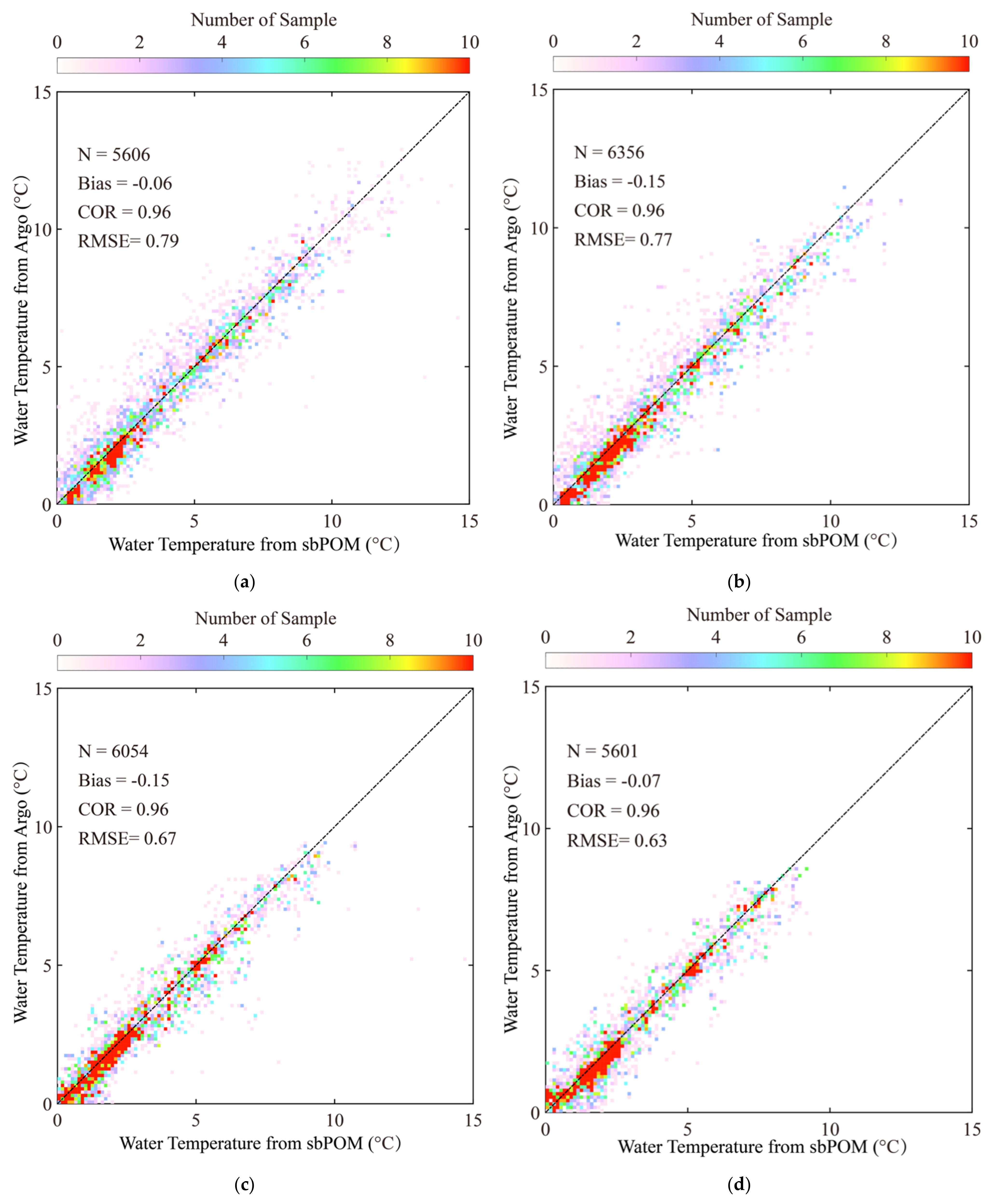
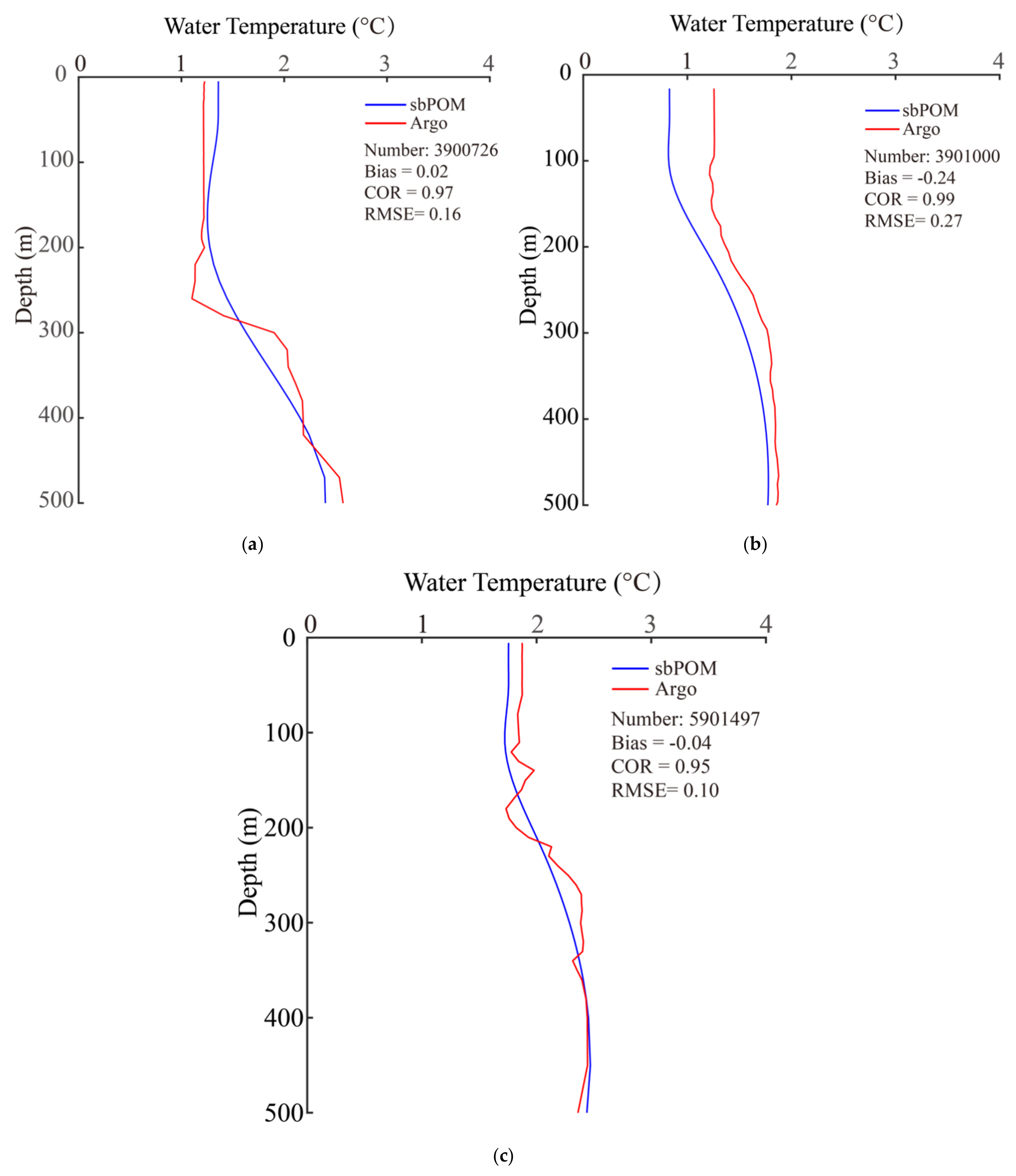
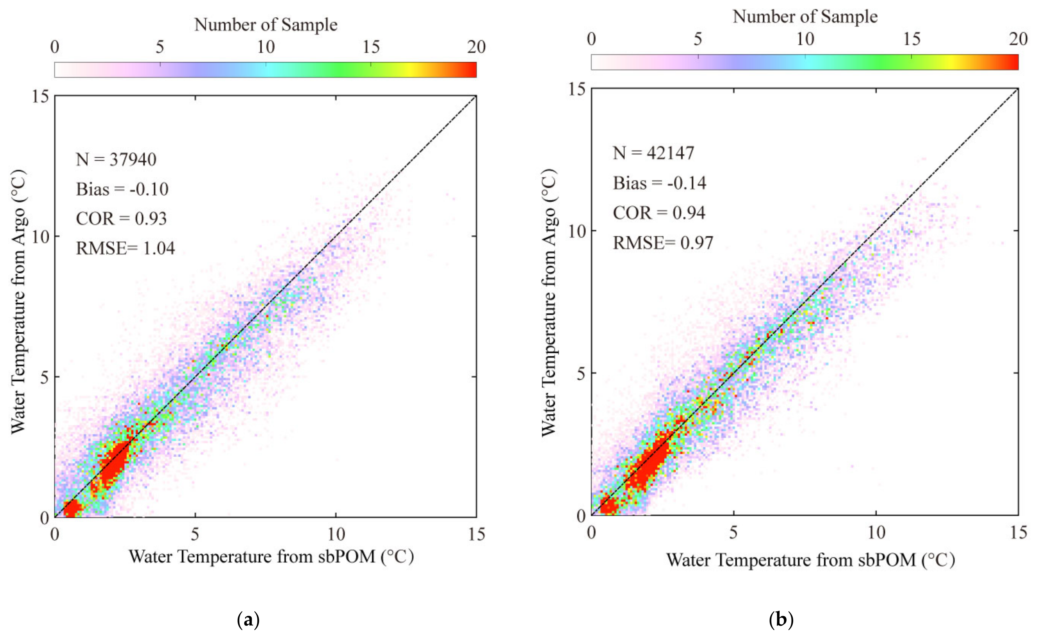
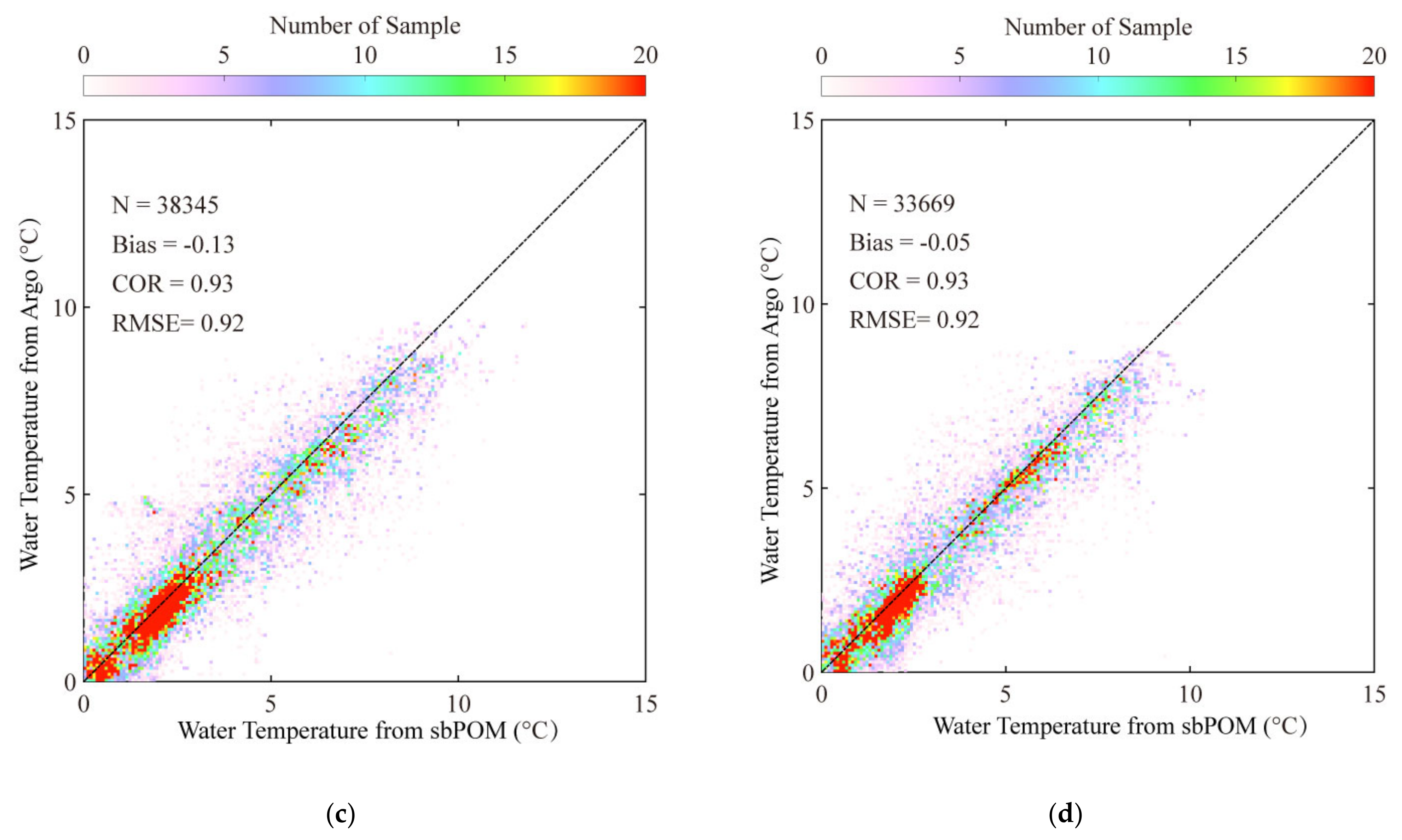
3.1. Validation of sbPOM-Simulated Water Temperature

In order to study the impact of waves on water temperature, the SST and wave simulation results from two ocean models were analyzed. The statistical analysis of the sbPOM-simulated water temperatures via comparison with the collocated measurements from Argo buoys is shown in Figure 9, i.e., in (a) January 2009, (b) March 2009, (c) July 2009, and (d) September 2009. It was found that the RMSE of the water temperature was less than 0.8 °C with a COR of 0.96. Specifically, the accuracy of the water temperature was relatively better in January and March than in July and September. The monthly average WW3-simulated wave distributions in (a) January 2009, (b) March 2009, (c) July 2009, and (d) September 2009 are presented in Figure 10. In general, the wave distribution of the WW3-simulated SWHs (>3 m) in winter and spring (January and March) were larger than those in summer and autumn (July and September), especially for SWHs of less than 1 m in the Antarctic Ocean in January. Based on this, we conclude that including the four terms induced by waves improved the accuracy of the temperature simulation.

The vertical profile of the simulated water temperature for water depths of up to 500 m and the data collocated from three Argo buoys (IDs: 3900726, 3901000, and 5901497) located in the Pacific Ocean, Atlantic Ocean, and Indian Ocean, which were acquired on 1 September 2009, are shown in Figure 11. Specifically, the geographic locations of the three Argo buoys in Figure 11a–c are (262° E, 61° S), (320° E, 51° S), and (43° E, 55° S), respectively. It can be clearly observed that the vertical profiles of the sbPOM-simulated water temperature are consistent with those obtained from the three Argo buoys with correlation coefficient (COR) of >0.95 and an RMSE of <0.3 °C. The comparison of water temperature between sbPOM-simulated results and the measurements from the available Argo buoys in Figure 5 on 1 December 2009 is listed in

Table 2. Validation of the sbPOM-simulated results against the available Argo buoys in Figure 5 on 1 December 2009.

Argo ID	RMSE (°C)	COR	Bias
5900894	0.94	0.85	0.27
5901178	0.35	0.96	−0.08
5901427	0.15	0.96	−0.14
5902119	0.44	0.97	−0.17
3901000	0.27	0.99	−0.24
5901448	0.36	0.96	−0.21
5901717	0.71	0.70	0.12
5901718	0.34	0.95	0.02
2900121	0.77	0.88	−0.37
5901495	0.31	0.86	0.16
5901497	0.10	0.95	−0.04
5901699	0.31	0.82	−0.24
5901725	0.36	0.97	0.05
5901726	0.89	0.92	−0.58
5902104	0.74	0.98	−0.50

, yielding a correlation coefficient (COR) of >0.85 and an RMSE of <0.94 °C.

Moreover, the statistical analysis of the sbPOM-simulated water temperatures compared with the collocated measurements from the Argo buoys is shown in Figure 12, e.g., in (a) January 2011–2015, (b) March 2011–2015, (c) July 2011–2015, and (d) September 2011–2015. It was found that the RMSE of the water temperature was less than 1.0 °C with a COR of 0.92. Specifically, the accuracy of the water temperature was relatively better in January and March than in July and September. In this sense, it was concluded that the sbPOM-simulated water temperature was reliable for this study.

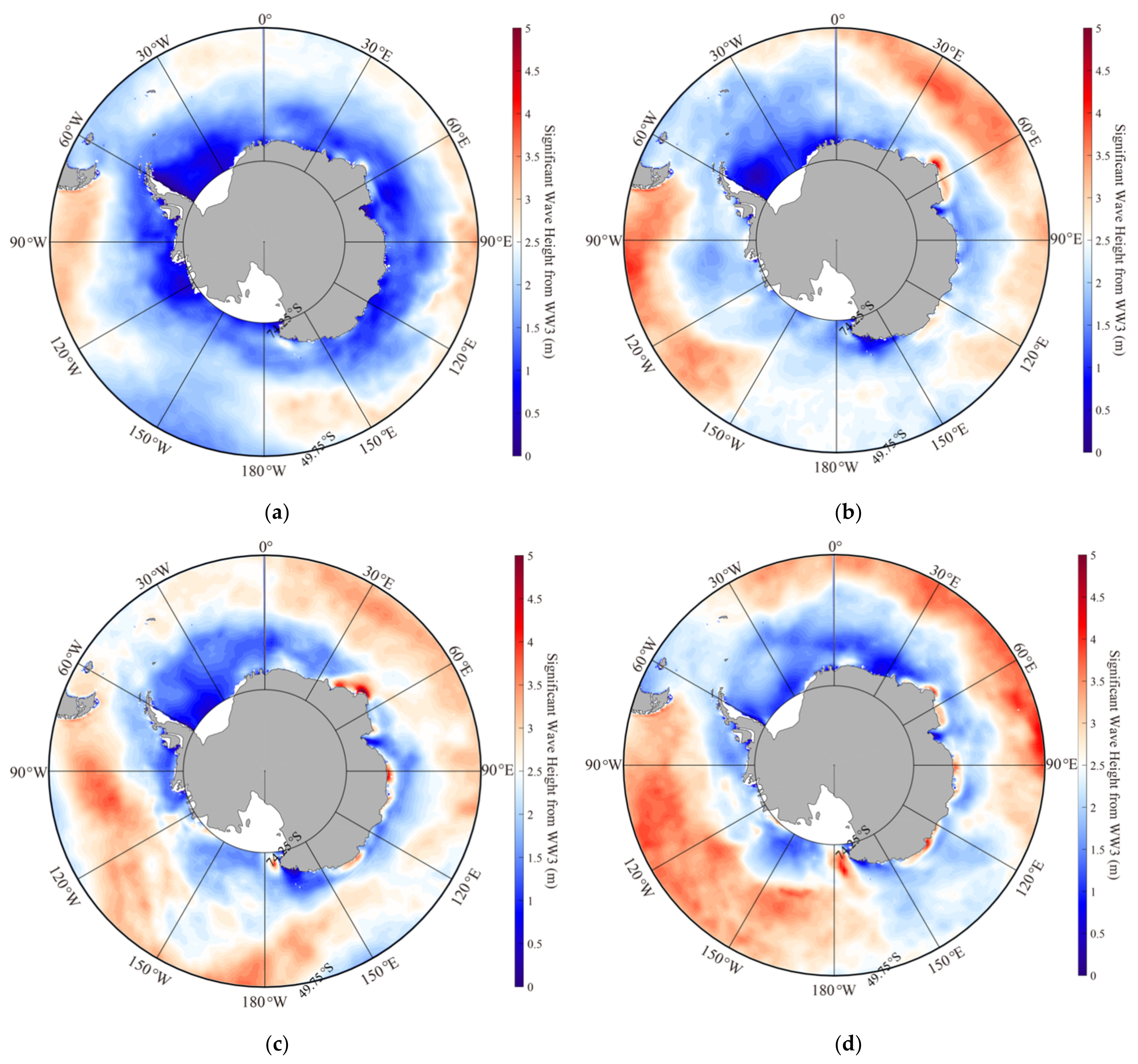
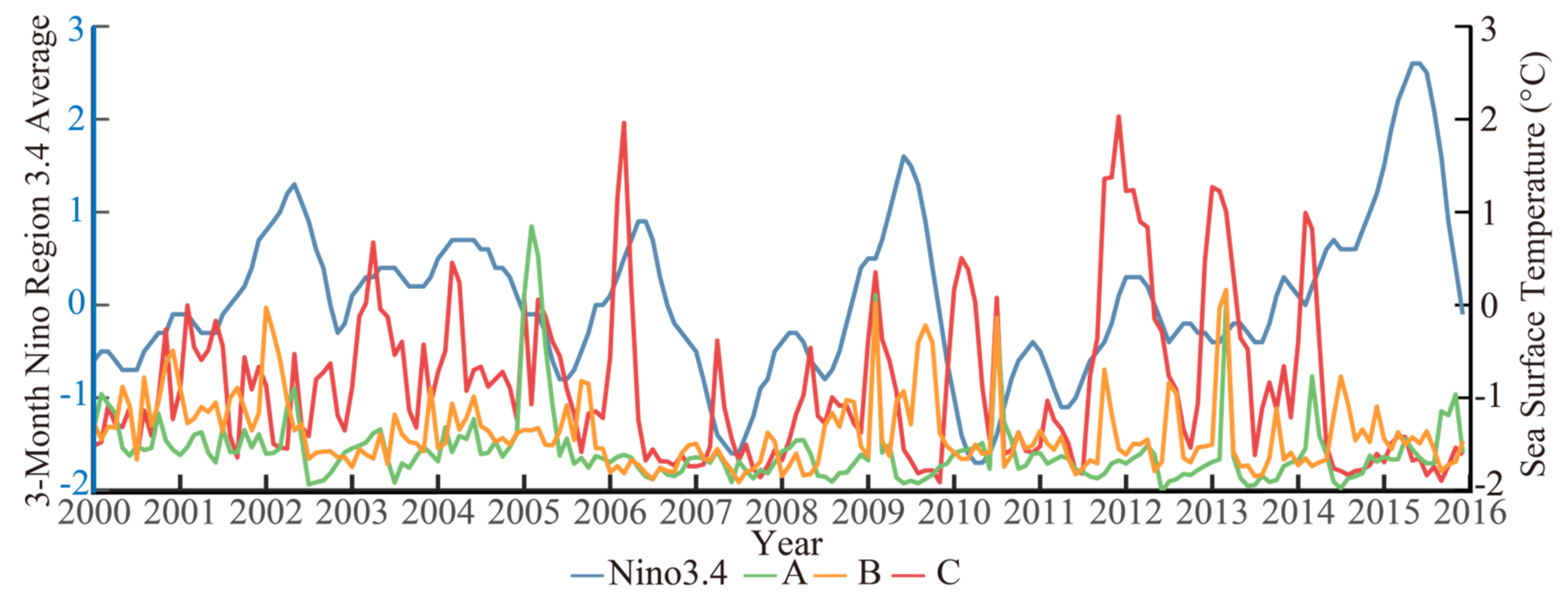
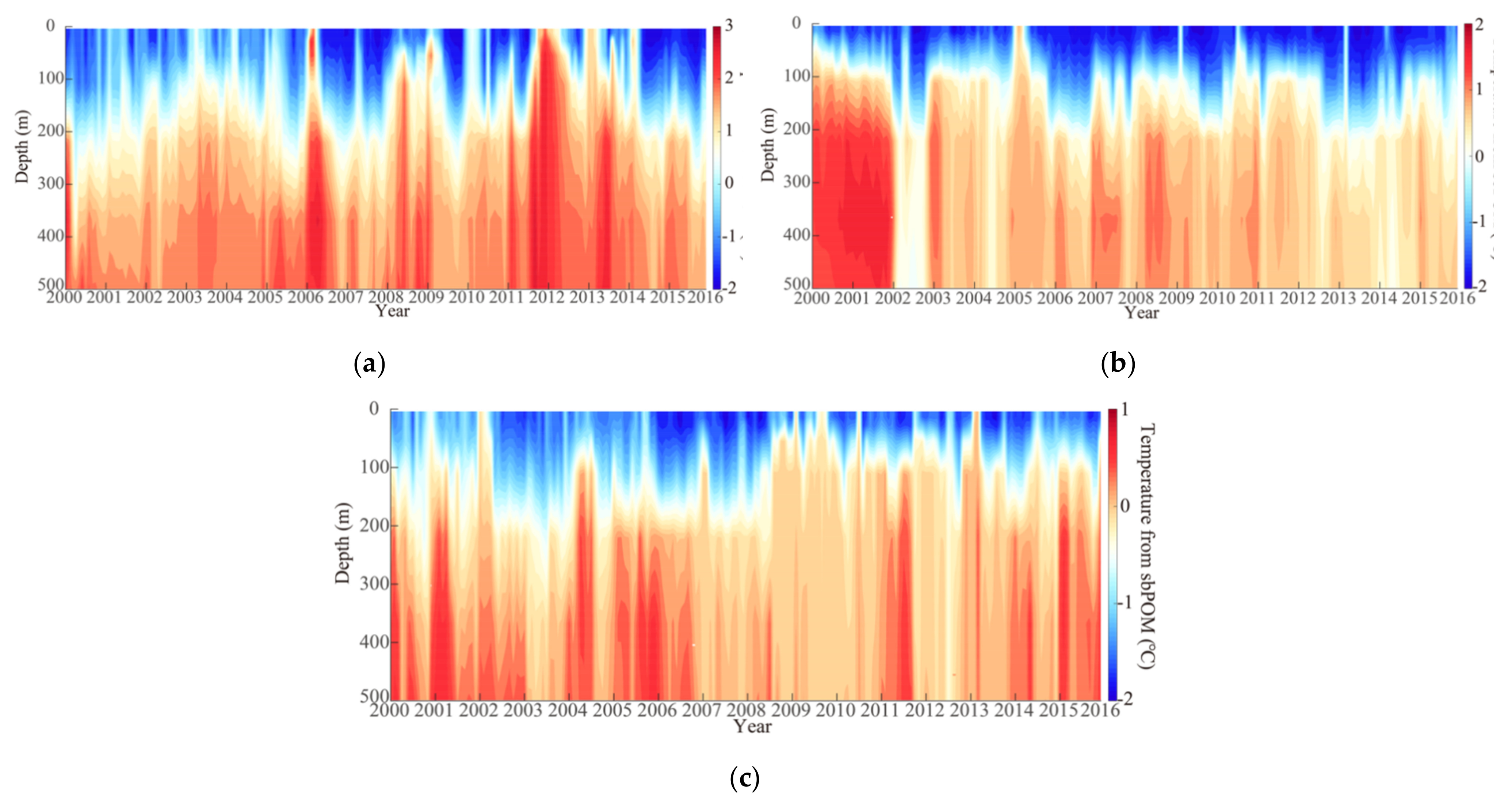
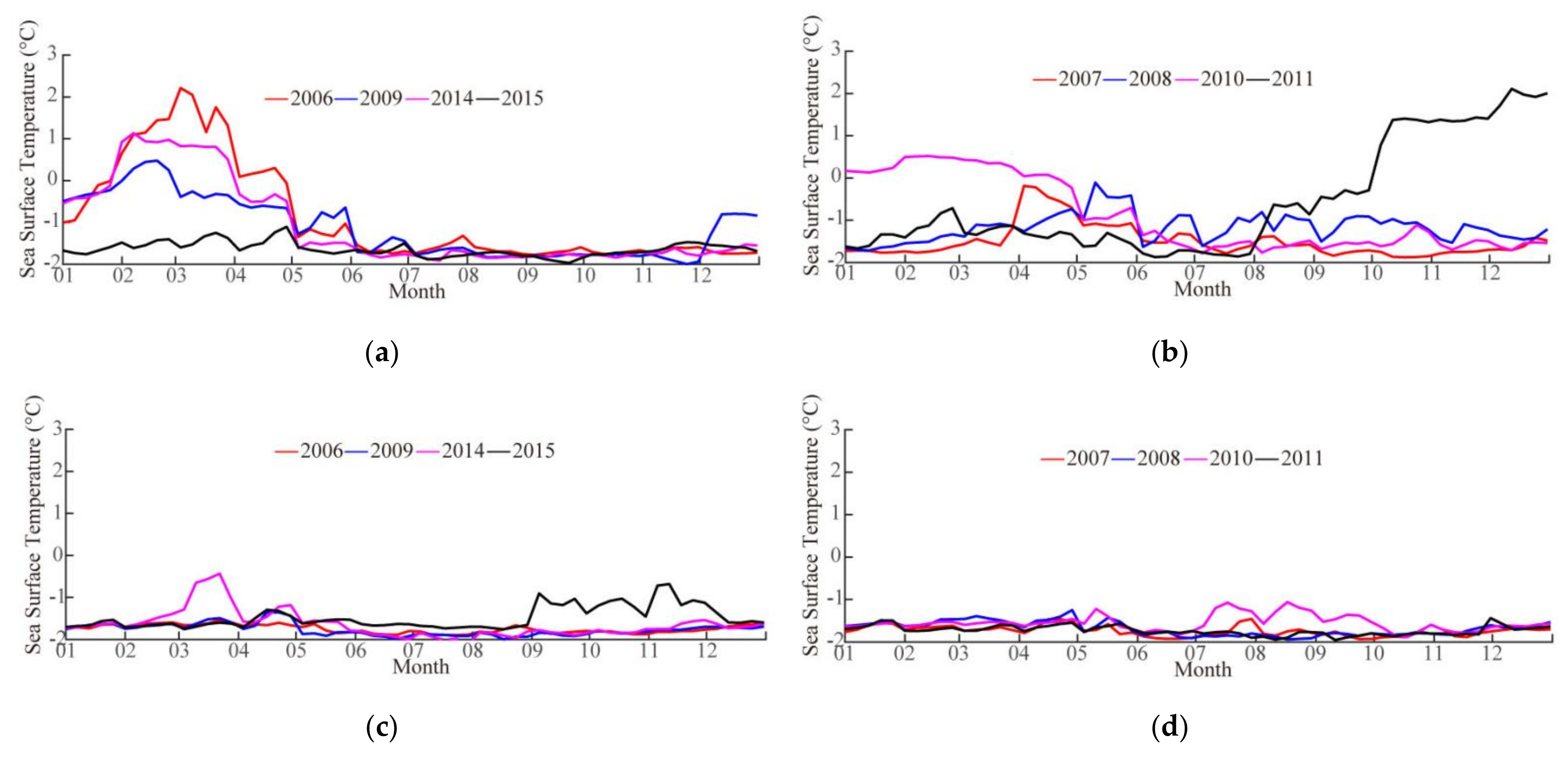
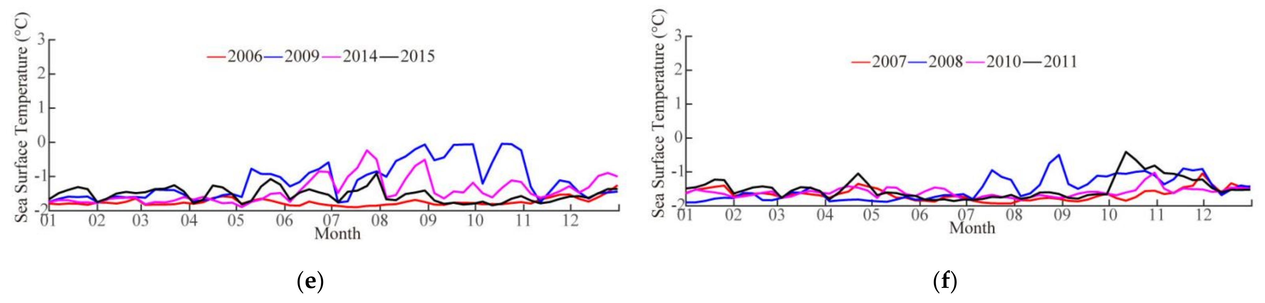
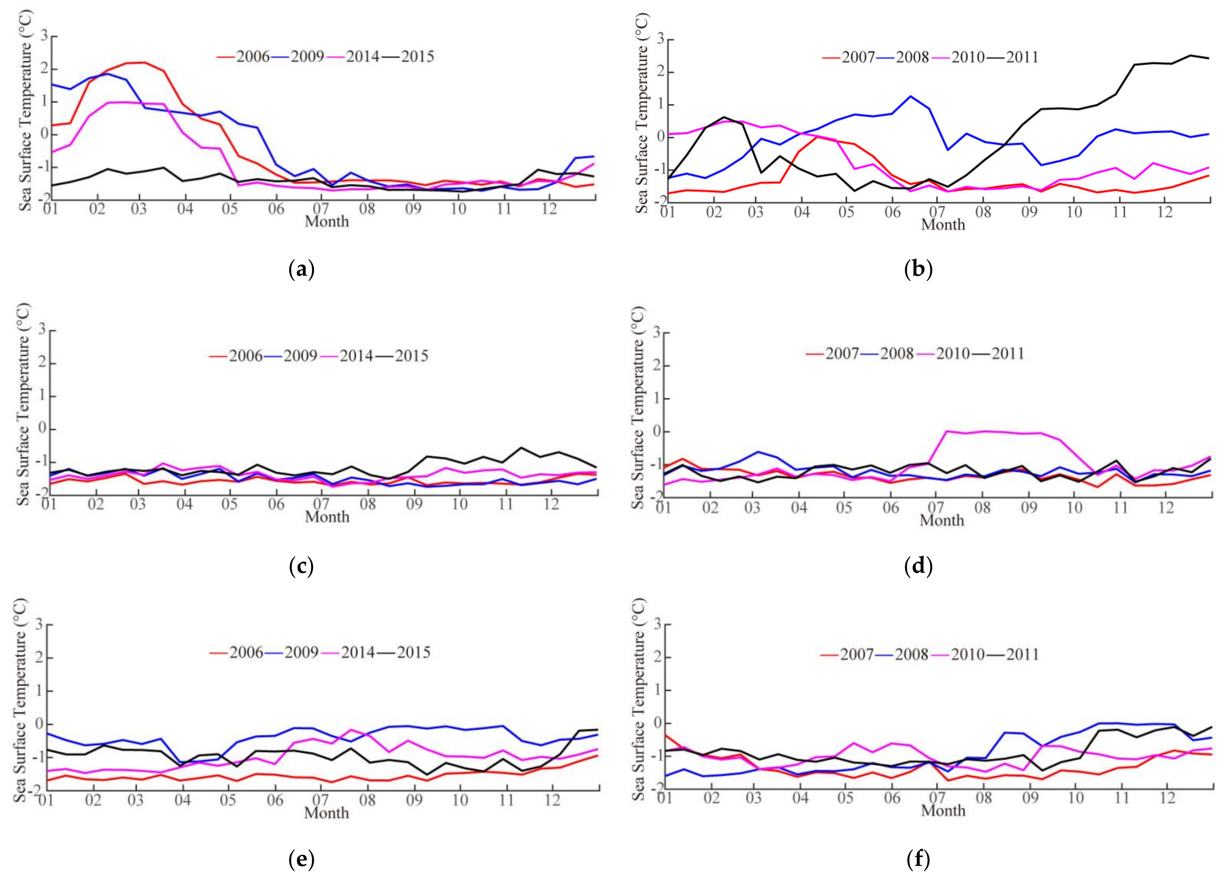
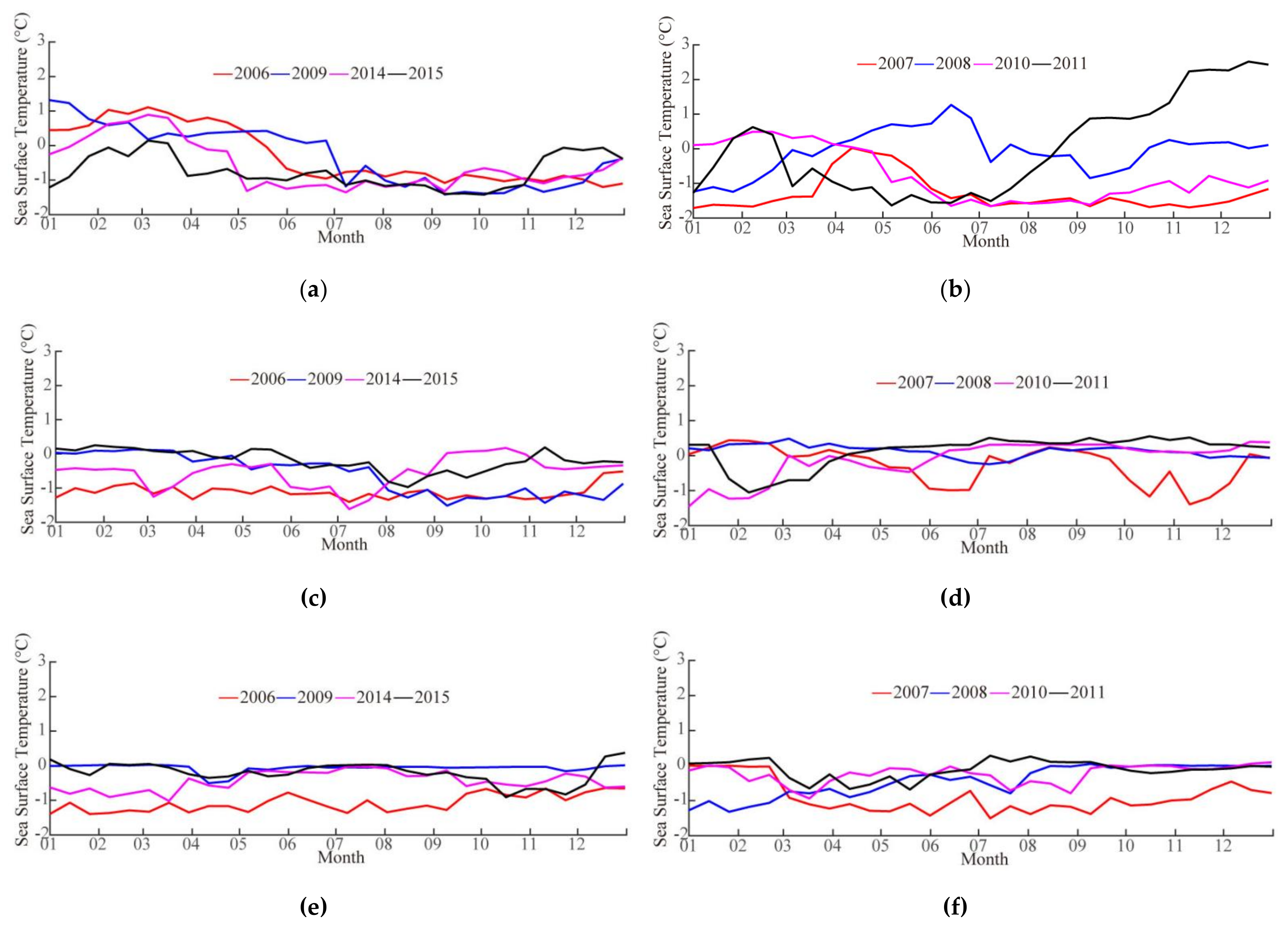
3.2. Variations of Water Temperature

The annual variations in the sbPOM-simulated water temperatures from January 2000 to December 2016 with the oceanic Nino index were analyzed at three locations at the same latitude (points A–C in Figure 1), as shown in Figure 13. Generally, the SST oscillates during the year; however, the SST was higher in the Pacific Ocean and Atlantic Ocean than in the Indian Ocean. The variation trend of SST had a similar trend of the oceanic Nino index, e.g., the high SST with the occurrence of the El Nino or La Nina events. Interestingly, the SST rapidly increased to 2 °C at location A in the Pacific Ocean in specific years, e.g., in 2006–2009 and 2012–2014. This type of behavior is worthy of further investigation.

Figure 14 shows the vertical profiles of the sbPOM-simulated water temperature at locations A–C. It can be clearly seen that the water temperature increases with increasing depth. This finding is consistent with those of previous studies [44], that is, the temperature of the Antarctic bottom is increasing. At location C in the Indian Ocean, the depth of the cool water temperature (<0 °C) was about 200 m in 2000–2008, as well as in locations A and B; however, the depth has decreased to 100 m since 2008. In this sense, the temperature of the Antarctic Surface Water (<500 m) in the Indian Ocean has warmed significantly since 2008, but the maximum water temperature was up to 1 °C. In location A in the Pacific Ocean and location B in the Atlantic Ocean, the occurrence of El Nino and La Nina events can cause water temperature warming in specific years.

4. Discussion

As was mentioned by Zhang et al. [53], statistical analysis revealed that El Nino events occurred in 2006 (weak), 2009 (moderate), 2014 (weak), and 2015 (very strong), and La Nina events occurred in 2007 (strong), 2008 (weak), 2010 (strong), and 2011(moderate). In these years, the SST increased significantly (Figure 11). In this section, the seasonal variations in the water temperature at locations A–C during El Nino and La Nina events are discussed.

Figure 15a,c,e show the seasonal variations in the SST at locations A–C during the El Nino events. Similarly, Figure 15b,d,f show the variations in the SST at locations A–C during the La Nina events. The seasonal variations in the temperature of the Antarctic surface water at depths of 50 m and 100 m are also shown in Figure 16 and Figure 17, respectively. It can be seen that the SST at location A in the Pacific Ocean increased from January to March and then gradually decreased until June. In contrast, La Nina had a complex impact on the seasonal variations in the SST at location A in the Pacific Ocean, e.g., cooling of the SST from January to July in 2010 and warming of the SST from August to December in 2011. In particular, with the increasing intensity of the El Nino events, the amplitude of water warming from January to July was reduced and a similar trend of the La Nina events from September to December was also found. At location B in the Atlantic Ocean, the intensity of the El Nino and La Nina events caused specific SST increases in specific months, e.g., September to December in 2015 and July to October in 2010; however, there was no trend in the seasonal variations in the water temperature at 100 m of water depth. With the El Nino and La Nina events occurring, the depth of zonal mean tropical Pacific thermocline and the local wind field changed and then influenced the intensity of the North Atlantic thermohaline circulation and the patterns of the Pacific sea surface temperature [54]. At location C in the Indian Ocean, SST increases at the El Nino and La Nina events were also found, similar to that in the Pacific Ocean; however, the amplitude of water warming in the Indian Ocean (~1 °C) was less than ~3 °C in the Pacific Ocean. Due to the effort of the global thermohaline circulation, the water-generating temperature warming at the Antarctic bottom is revealed at the El Nino and La Nina events [26]. The floating of the Antarctic bottom water leads to the increase in temperature of the Antarctic surface water. Collectively, the variations in the water temperature in spring and summer in the Pacific Ocean were sensitive to the El Nino events. Moreover, it was also found that the increasing intensity of the El Nino and La Nina events could reduce the water warming in the Pacific Ocean.

5. Conclusions

With rapid global change, more sea ice is melting year by year in the Arctic Ocean [55], resulting in increased water temperatures and the growth of sea fetch. In contrast, the coverage of sea ice in the Antarctic Ocean is expanding and observations have revealed that the temperature of the Antarctic bottom water is increasing due to variations in the Antarctic circumpolar current. In fact, the water temperature of the upper layer is affected by the energy exchange in the vertical direction. Therefore, in this study, the variations in the Antarctic surface water (<500 m) were investigated in the context of El Nino and La Nina events.

In this study, two numerical ocean models, namely the WW3 and sbPOM, were offline coupled to simulate the water temperature in the Antarctic Ocean. The sea surface waves were simulated using the WW3 model, in which the ERA-5 winds and NCEP CFSv2 currents were treated as the forcing field. The validation of the simulations against measurements from the Jason-2 altimeter produced an RMSE 0.39 m for the SWH with a 0.30-m bias. Four wave-induced terms—breaking waves, nonbreaking waves, radiation stress, and Stokes drift—were calculated using the WW3-simulated waves. These wave-induced terms were included in the water temperature simulation using the sbPOM. The sbPOM-simulated water temperatures were compared with the measurements collocated from Argo buoys in January, March, July, and September in 2009, yielding a COR of >0.96 and an RMSE of <0.8 °C for the water temperature. It was found that the accuracy of the water temperature was improved by including the four wave-induced terms, especially for the high WW3-simulated SWH in July and September. As mentioned in [9], wave-induced Stokes transport in the China Seas gradually increased between 1987 and 2020. The term of wave should be included in the SST simulation by sbPOM at specific regions, e.g., the Arctic Ocean [5] and China Seas, and at extreme events, e.g., typhoon and hurricane.

The analysis of the annual variations in the sbPOM-simulated water temperatures revealed that the SST increased in the Antarctic Ocean in specific years, which is related to the occurrences of El Nino and La Nina events. The depth of the cool water in the Indian Ocean decreased to 100 m, although the maximum water temperature was up to 1 °C, which is less than the maximum water temperatures of 3 °C and 2 °C in the Pacific Ocean and the Atlantic Ocean, respectively. The seasonal variations in the water temperature at depths of 0 m, 50 m, and 100 m were qualitatively studied further in the context of El Nino and La Nina events. It was found that the Pacific Ocean was more sensitive to El Nino events, i.e., with increasing SST from January to March and decreasing SST until June. Moreover, the increasing intensity of the El Nino and La Nina events could reduce water warming in the Pacific Ocean. However, El Nino and La Nina events had smaller impacts on seasonal variations in the water temperature of the Atlantic and Indian oceans.

In the future, quantitative analysis on the amplitude of the increase in the water temperature of the Antarctic Ocean, considering the intensity of the El Nino and La Nina events, will be further studied.

References

1. Stopa, J.E.; Fabrice, A.; Fanny, G.A. Wave climate in the Arctic 1992–2014: Seasonality and trends. Cryosphere 2016, 10, 1605–1629. [Google Scholar] [CrossRef] [Green Version]
2. Jacka, T.H.; Budd, W.F. Detection of temperature and sea-ice-extent changes in the Antarctic and Southern Ocean, 1949–1996. Ann. Glaciol. 1998, 27, 553–559. [Google Scholar] [CrossRef] [Green Version]
3. Martinson, Y. Antarctic sea ice extent variability and its global connectivity. J. Clim. 2000, 13, 1697–1717. [Google Scholar]
4. Kiefer, T.; Mccave, I.N.; Elderfield, H. Antarctic control on tropical Indian Ocean sea surface temperature and hydrography. Geophys. Res. Lett. 2006, 33, L24612. [Google Scholar] [CrossRef]
5. Shao, W.Z.; Yu, W.P.; Jiang, X.W.; Shi, J.; Wei, Y.L.; Ji, Q.Y. Analysis of wave distributions using the WAVEWATCH-III model in the Arctic Ocean. J. Ocean U. China 2022, 21, 15–27. [Google Scholar] [CrossRef]
6. Stammer, D. Response of the global ocean to Greenland and Antarctic ice melting. J. Geophys. Res. 2008, 113, C06022. [Google Scholar] [CrossRef] [Green Version]
7. Orsi, A.H.; Johnson, G.C.; Bullister, J.L. Circulation, mixing, and production of Antarctic bottom water. Progr. Oceanogr. 1999, 4, 55–109. [Google Scholar] [CrossRef]
8. Cathles, L.M.; Okal, E.A.; Macayeal, D.R. Seismic observations of sea swell on the floating ross ice shelf, Antarctica. J. Geophys. Res. 2009, 114, F02015. [Google Scholar] [CrossRef] [Green Version]
9. Sun, Z.; Shao, W.; Wang, W.; Zhou, W.; Yu, W.; Shen, W. Analysis of wave-induced Stokes transport effects on sea surface temperature simulations in the Western Pacific Ocean. J. Mar. Sci. Eng. 2021, 9, 834. [Google Scholar] [CrossRef]
10. Ohshima, K.I.; Takizawa, T.; Ushio, S.; Kawamura, T. Seasonal variations of the Antarctic coastal ocean in the vicinity of Lützow-Holm Bay. J. Geophys. Res. 1996, 101, 20617–20628. [Google Scholar] [CrossRef]
11. Holland, P.R.; Kwok, R. Wind-driven trends in Antarctic sea-ice drift. Nature 2012, 5, 872–875. [Google Scholar] [CrossRef]
12. Fletcher, J.O.; Radok, U.; Slutz, R. Climatic signals of the Antarctic ocean. J. Geophys. Res. 1982, 87, 4269. [Google Scholar] [CrossRef]
13. And, P.F.; Zambianchi, E. Near-surface structure of the Antarctic circumpolar current derived from world ocean circulation experiment drifter data. J. Geophys. Res. 2011, 116, C05003. [Google Scholar]
14. The WAMDI Group. The WAM model—A third generation ocean wave prediction model. J. Phys. Oceanogr. 1998, 18, 1775–1810. [Google Scholar]
15. Tolman, L. A third-generation model for wind waves on slowly varying, unsteady, and inhomogeneous depths and currents. J. Phys. Oceanogr. 1991, 21, 782–797. [Google Scholar] [CrossRef]
16. Holthuijsen, L. The continued development of the third-generation shallow water wave model ‘SWAN’. Tu Delft Dep. Hydraul. Eng. 2001, 32, 185–186. [Google Scholar]
17. Wang, Z.F.; Gong, Y.J.; Cui, J.N.; Dong, S.; Wu, K.J. Effect of the drag coefficient on a typhoon wave model. J. Oceanol. Limnol. 2019, 37, 1795–1804. [Google Scholar] [CrossRef]
18. Zhou, L.M.; Li, Z.B.; Mu, L.; Wang, A.F. Numerical simulation of wave field in the South China Sea using WAVEWATCH III. Chin. J. Oceanol. Limn. 2014, 37, 656–664. [Google Scholar] [CrossRef]
19. Zheng, K.W.; Sun, J.; Guan, C.L.; Shao, W.Z. Analysis of the global swell and wind-sea energy distribution using WAVEWATCH III. Adv. Meteorol. 2016, 7, 8419580. [Google Scholar] [CrossRef] [Green Version]
20. Wadhams, P.; Squire, V.A.; Goodman, D.J.; Cowan, A.M.; Moore, S.C. The attenuation rates of ocean waves in the marginal ice zone. J. Geophys. Res. 1988, 93, 6799–6818. [Google Scholar] [CrossRef]
21. Li, Z.L.; Wen, P. Comparison between the response of the Northwest Pacific Ocean and the South China Sea to Typhoon Megi (2010). Adv. Atmos. Sci. 2017, 34, 79–87. [Google Scholar] [CrossRef]
22. Gao, J.S.; Chen, B.; Shi, M.C. Summer circulation structure and formation mechanism in the Beibu Gulf. Sci. China Earth Sci. 2015, 58, 286–299. [Google Scholar] [CrossRef]
23. Jordi, A.; Wang, D.P. Sbpom: A parallel implementation of Princenton ocean model. Environ. Modell. Softw. 2012, 38, 59–61. [Google Scholar] [CrossRef] [Green Version]
24. Sun, Z.F.; Shao, W.Z.; Yu, W.P.; Li, J. A Study of wave-induced effects on sea surface temperature simulations during typhoon events. J. Mar. Sci. Eng. 2021, 9, 622. [Google Scholar] [CrossRef]
25. Liu, N.; Zhang, Z.H.; Chen, H.X.; Lin, L.N. Western Indian Ocean SST signal and anomalous Antarctic sea-ice concentration variation. Acta Oceanol. Sin. 2011, 30, 9–13. [Google Scholar] [CrossRef]
26. Haumann, F.A.; Gruber, N.; Münnich, M.; Frenger, I.; Kern, S. Sea-ice transport driving Southern Ocean salinity and its recent trends. Nature 2016, 537, 89–92. [Google Scholar] [CrossRef]
27. The WAVEWATCH III Development Group (WW3DG). User Manual and System Documentation of WAVEWATCH III; Version 5.16; Tech. Note 329; NOAA/NWS/NCEP/MMAB: College Park, MD, USA, 2016; Volume 276, p. 326. [Google Scholar]
28. Hu, Y.Y.; Shao, W.Z.; Shi, J.; Sun, J.; Cai, L.N. Analysis of the typhoon wave distribution simulated in WAVEWATCH-III model in the context of Kuroshio and wind-induced current. J. Oceanol. Limnol. 2020, 38, 1692–1710. [Google Scholar] [CrossRef]
29. Sheng, Y.X.; Shao, W.Z.; Li, S.Q.; Zhang, Y.M.; Yang, H.W.; Zuo, J.C. Evaluation of typhoon waves simulated by WaveWatch-III model in shallow waters around Zhoushan islands. J. Ocean Univ. China 2019, 18, 365–375. [Google Scholar] [CrossRef]
30. Shao, W.Z.; Sheng, Y.X.; Li, H.; Shi, J.; Ji, Q.Y.; Tan, W.; Zuo, J.C. Analysis of wave distribution simulated by WAVEWATCH-III Model in typhoons passing Beibu Gulf, China. Atmosphere 2018, 9, 265. [Google Scholar] [CrossRef] [Green Version]
31. Barbariol, F.; Davison, S.; Falcieri, F.M.; Ferretti, R.; Ricchi, A.; Sclavo, M.; Benetazzo, A. Wind Waves in the Mediterranean Sea: An ERA5 Reanalysis Wind-Based Climatology. Front. Mar. Sci. 2021, 8, 760614. [Google Scholar] [CrossRef]
32. Yang, Z.H.; Shao, W.Z.; Ding, Y.; Shi, J.; Ji, Q.Y. Wave simulation by the SWAN model and FVCOM considering the Sea-water-level term around the Zhoushan islands. J. Mar. Sci. Eng. 2020, 8, 783. [Google Scholar] [CrossRef]
33. Saha, S.; Moorthi, S.; Wu, X.R.; Wang, J.D.; Nadiga, S.; Tripp, P.; Behringer, D.; Hou, Y.T.; Chuang, H.Y.; Iredell, M.; et al. The NCEP Climate Forecast System Version 2. J. Clim. 2014, 27, 2185–2208. [Google Scholar] [CrossRef]
34. Bryan, K. A numerical method for the study of the circulation of the World Ocean. J. Comput. Phys. 1969, 4, 347–376. [Google Scholar] [CrossRef]
35. Robinson, A.R.; Walstad, L.J. The Harvard open ocean model: Calibration and application to dynamical process, forecasting, and data assimilation studies. Appl. Numer. Math. 1987, 3, 89–131. [Google Scholar] [CrossRef]
36. Zhang, J.; Schmitt, R.W.; Huang, R.X. Sensitivity of the GFDL modular ocean model to parameterization of double-diffusive processes. J. Phys. Oceanogr. 1998, 28, 589–605. [Google Scholar] [CrossRef]
37. Jones, P.W.; Worley, P.H.; Yoshida, Y.; Iii, J.; Levesque, J. Practical performance portability in the parallel ocean program (POP). Concurr. Comp. Pract. Exp. 2010, 17, 1317–1327. [Google Scholar] [CrossRef]
38. Gerdes, R. A primitive equation ocean circulation model using a general vertical coordinate transformation: 1. Description and testing of the model. J. Geophys. Res. 1993, 98, 14683–14701. [Google Scholar] [CrossRef]
39. Robertson, R.; Padman, L.; Levine, M.D. A correction to the baroclinic pressure gradient term in the Princeton Ocean Model. J. Atmos. Ocean. Technol. 2001, 18, 1068–1075. [Google Scholar] [CrossRef] [Green Version]
40. Kamenkovich, V.M.; Nechaev, D.A. On the time-splitting scheme used in the Princeton Ocean Model. J. Comput. Phys. 2009, 228, 2874–2905. [Google Scholar] [CrossRef]
41. Chen, C.; Huang, H.; Beardsley, R.C.; Liu, H.; And, Q.X.; Cowles, G. A finite volume numerical approach for coastal ocean circulation studies: Comparisons with finite difference models. J. Geophys. Res. 2007, 112, C03018. [Google Scholar] [CrossRef]
42. Shchepetkin, A.F.; McWilliams, J.C. The Regional Ocean Modeling System: A split-explicit, free-surface, topography following coordinates ocean model. Ocean Model. 2005, 9, 347–404. [Google Scholar] [CrossRef]
43. Bleck, R. An oceanic general circulation model framed in hybrid isopycnic-cartesian coordinates. Ocean Model. 2002, 4, 55–88. [Google Scholar] [CrossRef]
44. Chassignet, E.P.; Smith, L.T.; Halliwell, G.R.; Bleck, R. North Atlantic simulations with the hybrid coordinate ocean model (HYCOM): Impact of the vertical coordinate choice, reference pressure, and thermobaricity. J. Phys. Oceanogr. 2003, 3, 2504–2526. [Google Scholar] [CrossRef] [Green Version]
45. Bleck, R.; Smith, L.T. A wind-driven isopycnic coordinate model of the north and equatorial Atlantic Ocean: 1. Model development and supporting experiments. J. Geophys. Res. 1990, 95, 3273–3285. [Google Scholar] [CrossRef]
46. Chen, C.; Liu, H.; Beardsley, C.R. An unstructured, finite-volume, three-dimensional, primitive equation ocean model: Application to coastal ocean and estuaries. J. Atmos. Ocean. Technol. 2003, 20, 159–186. [Google Scholar] [CrossRef]
47. Sheng, Y.P.; Zhang, Y.; Paramygin, V.A. Simulation of storm surge, wave, and coastal inundation in the Northeastern Gulf of Mexico region during Hurricane Ivan in 2004. Ocean Model. 2010, 35, 314–331. [Google Scholar] [CrossRef]
48. Zhang, Y.; Baptista, A.M. SELFE: A semi-implicit Eulerian-Lagrangian finite-element model for cross-scale ocean circulation. Ocean Model. 2008, 21, 71–96. [Google Scholar] [CrossRef]
49. Guan, C.L.; Hu, W.; Sun, J.; Li, R.L. The whitecap coverage model from breaking dissipation parametrizations of wind waves. J. Geophys. Res. 2007, 112, C05013. [Google Scholar] [CrossRef] [Green Version]
50. And, H.H.; Wang, J. Modeling effects of tidal and wave mixing on circulation and thermohaline structures in the Bering sea: Process studies. J. Geophys. Res. 2010, 115, C01006. [Google Scholar]
51. Wu, L.; Chen, C.; Guo, P.; Shi, M.; Qi, J.; Ge, J. A FVCOM-based unstructured grid wave, current, sediment transport model, I. model description and validation. J. Ocean Univ. China 2011, 10, 1–8. [Google Scholar] [CrossRef]
52. Mesquita, O.N.; Kane, S.; Gollub, J.P. Transport by capillary waves: Fluctuating stokes drift. Phys. Rev. A 1992, 45, 3700. [Google Scholar] [CrossRef] [Green Version]
53. Zhang, W.; Zhou, X.; Hsu, P.C.; Liu, F. Diversity of East China Summer rainfall change in post-El Nio summers. Front. Earth Sci. 2020, 8, 595548. [Google Scholar] [CrossRef]
54. Duan, C.; Dong, S.; Xie, Z.; Wang, Z. Temporal variability and trends of sea ice in the Kara sea and their relationship with atmospheric factors. Polar Sci. 2019, 20, 136–147. [Google Scholar] [CrossRef]
55. Timmermann, A.; An, S.I.; Krebs, U.; Goosse, H. ENSO Suppression due to weakening of the North Atlantic thermohaline circulation. J. Clim. 2005, 18, 3122–3139. [Google Scholar] [CrossRef] [Green Version]
Figure 1. The water depth map from the general bathymetry chart of the oceans (GEBCO) with a 0.1° horizontal resolution. The three red spots are selected for analysis in the Pacific Ocean, Indian Ocean and Atlantic Ocean. The red lines represent the boundaries of the three oceans.
Jmse 10 00287 g001
Figure 2. The 0.25° gridded European Centre for Medium-Range Weather Forecasts (ECMWF) reanalysis (ERA-5) wind speed map at 18:00 UTC on 1 January 2009.
Jmse 10 00287 g002
Figure 3. The 0.5° gridded current speed map from the National Centers for Environmental Prediction (NCEP) Climate Forecast System Version 2 (CFSv2) at 18:00 UTC on 1 January 2009.
Jmse 10 00287 g003
Figure 4. The flow chart of the coupling method of the two models.
Jmse 10 00287 g004
Figure 5. (a) The monthly average sea surface temperature; and (b) the average sea surface salinity from the Simple Ocean Data Assimilation (SODA) data for January 2009.
Jmse 10 00287 g005
Figure 6. The National Centers for Environmental Prediction (NCEP) reanalysis total heat flux (latent heat flux, sensible heat flux, long-wave radiation, and solar radiation) map at 18:00 UTC on 1 December 2009, in which the red triangles represent the geographic locations of the Argo buoys.
Jmse 10 00287 g006
Figure 7. The significant wave height (SWH) map at 18:00 UTC on 1 December 2009 obtained using the WAVEWATCH-III (WW3) model. The colored rectangles represent the SWH measured by the footprints of Jason-2 altimeter.
Jmse 10 00287 g007
Figure 8. Comparison of the SWH simulated using the WW3 model and the measurements of the Jason-2 altimeter following the footprint for a 0.4 m bin between 0 and 8 m, in which the error bars represent the standard deviations of each bin for the matchups.
Jmse 10 00287 g008
Figure 9. Comparison of the Argo-measured water temperature with the collocated samples from the sbPOM in (a) January 2009, (b) March 2009, (c) July 2009, and (d) September 2009.
Jmse 10 00287 g009
Figure 10. The monthly average WW3-simulated wave distributions in (a) January 2009, (b) March 2009, (c) July 2009, and (d) September 2009.
Jmse 10 00287 g010
Figure 11. (a) The vertical water temperature profile on 1 September 2009 in the Pacific Ocean obtained from the Argo (ID: 3900726, 262° E, 61° S) and simulated using the sbPOM, (b) the vertical temperature profile obtained from an Argo (ID: 3901000, 320° E, 51° S) and simulated using the sbPOM and (c) the vertical temperature profile obtained from an Argo (ID: 5901497, 43° E, 55° S) and simulated using the sbPOM in the Indian Ocean.
Jmse 10 00287 g011
Figure 12. Comparison of the Argo-measured water temperature with the collocated samples from the sbPOM in (a) January 2011–2015, (b) March 2011–2015, (c) July 2011–2015, and (d) September 2011–2015.
Jmse 10 00287 g012aJmse 10 00287 g012b
Figure 13. The annual variations in the sbPOM-simulated SSTs from January 2000 to December 2016 at locations A–C (shown in Figure 1) with the 3-month Nino region 3.4 average (Nino 3.4 index), e.g., spot A in the Pacific Ocean, spot B in the Atlantic Ocean and spot C in the Indian Ocean.
Jmse 10 00287 g013
Figure 14. Vertical profiles of the sbPOM-simulated water temperature from January 2000 to December 2016 at locations A–C (shown in Figure 1): (a) Location A in the Pacific Ocean, (b) Location B in the Atlantic Ocean and (c) Location C in the Indian Ocean.
Jmse 10 00287 g014
Figure 15. Seasonal variations in the SST during El Nino and La Nina events: (a) Location A in the Pacific Ocean during the events of El Nino; (b) Location A in the Pacific Ocean during La Nina events; (c) Location B in the Atlantic Ocean during El Nino events; (d) Location B in the Atlantic Ocean during La Nina events; (e) Location C in the Indian Ocean during El Nino events; and (f) Location C in the Indian Ocean during La Nina events.
Jmse 10 00287 g015aJmse 10 00287 g015b
Figure 16. Seasonal variations in the water temperature at a depth of 50 m during El Nino and La Nina events: (a) Location A in the Pacific Ocean during El Nino events; (b) Location A in the Pacific Ocean during La Nina events; (c) Location B in the Atlantic Ocean during El Nino events; (d) Location B in the Atlantic Ocean during La Nina events; (e) Location C in the Indian Ocean during El Nino events; and (f) Location C in the Indian Ocean during La Nina events.
Jmse 10 00287 g016
Figure 17. Seasonal variations in the water temperature at a depth of 100 m during El Nino and La Nina events: (a) Location A in the Pacific Ocean during El Nino events; (b) Location A in the Pacific Ocean during La Nina events; (c) Location B in the Atlantic Ocean during El Nino events; (d) Location B in the Atlantic Ocean during La Nina events; (e) Location C in the Indian Ocean during El Nino events; and (f) Location C in the Indian Ocean during La Nina events.
Jmse 10 00287 g017